
Stochastic Flocculation Model for Cohesive Sediment Suspended in Water

1
Department of Oceanography, Inha University, Incheon 402-751, Korea
2
Department of Civil Engineering, Chungnam National University, Daejeon 305-764, Korea
3
Department of Oceanography, Inha University, Incheon 402-751, Korea
*
Author to whom correspondence should be addressed.
Water 2015, 7(5), 2527-2541; https://doi.org/10.3390/w7052527
Submission received: 1 April 2015
/
Accepted: 18 May 2015
/
Published: 22 May 2015
Abstract
:Existing flocculation models for cohesive sediments are classified into two groups: population balance equation models (PBE) and floc growth models. An FGM ensures mass conservation in a closed system. However, an FGM determines only the average size of flocs, whereas a PBE has the capability to calculate a size distribution of flocs. A new stochastic approach to model the flocculation process is theoretically developed and incorporated into a deterministic FGM in this study in order to calculate a size distribution of flocs as well as the average size. A log-normal distribution is used to generate random numbers based on previous laboratory experiments. The new stochastic flocculation model is tested with three laboratory experiment results. It was found and validated with measured data that the new stochastic flocculation model has the capability to replicate a size distribution of flocs reasonably well under different sediment and carrier flow conditions. Three more distributions (normal; Pearson type 3; and generalized extreme value distributions) were also tested. From the comparison with results of different distribution functions, it is shown that a stochastic FGM using a log-normal distribution has a comparative advantage in terms of simplicity and accuracy.
1. Introduction
The flocculation process, a series of aggregation and disaggregation (so called breakup) processes, is one of the most important characteristics of suspended cohesive sediment such as mud and organic matter. Through the flocculation process, the size and density of cohesive sediment continuously vary, resulting in variation of settling velocity and particle response time. Because the settling velocity and particle response time significantly affect the advection and diffusion process of suspended sediment, an improved understanding of the flocculation process is paramount for cohesive sediment transport. Therefore, the flocculation process has been intensively studied. The flocculation process is mainly due to eletro- or biological-chemical attraction of fine sediment (e.g., [1]). When suspended particles collide with each other, there is a chance of aggregation by attraction. Collisions of suspended sediment are caused by Brownian motion, differential settling, and turbulent shear [2,3,4]. It has been concluded in many studies that turbulent shear is the dominant mechanism of suspended sediment collisions (e.g., [5,6]). Moreover, turbulent shear is considered as the main mechanism of floc breakup (e.g., [1,7,8]). Many laboratory studies on the effects of turbulent shear have been conducted utilizing a mixing tank and Couette viscometer in order to control the intensity of turbulent shear (e.g., [9,10,11,12]). From these studies, it is apparent that the flocculation process of aggregation (mainly due to particle collision) and breakup is significantly governed by turbulent shear.
With the aim of quantitatively modeling the flocculation process, many flocculation models have been proposed. Generally, flocculation models can be classified into two groups at present; a population balance equations model (PBE) and a floc growth model (FGM). A PBE, often called a size class flocculation model, is based on discrete size classes, and typically calculates the change of floc numbers in each size class (e.g., [13,14,15]). A PBE has the advantages of considering many mechanisms of flocculation and calculating a size distribution of flocs. However, a PBE is too numerically expensive to be combined with numerical sediment transport models [16] and demands many empirical parameters, increasing uncertainties. Moreover, a discrete PBE approach is limited in terms of ensuring the mass conservation of flocs in a closed system, although many schemes have been proposed to overcome this weakness (e.g., [17,18]). A FGM, often called a Lagrangian flocculation model, is a differential equation usually composed of two terms, an aggregation term and a breakup term, representing the increase in floc size due to aggregation and the decrease due to breakup, respectively. A FGM is simple enough to be combined with numerical sediment transport models. Furthermore, a FGM ensures the mass conservation of cohesive sediment in a closed system because it calculates the average size of flocs. Based on the collisional frequency equation of Levich [19] and dimensional analysis, Winterwerp [8] proposes a semi-empirical FGM under the assumption that the fractal dimension of flocs is constant. However, many studies show that the fractal dimension of natural flocs is variable (e.g., [20,21]). Based on Levich [19] and Khelifa and Hill [20], Son and Hsu [7] improved Winterwerp’s FGM [8] by adopting an empirical equation with a variable fractal dimension. However, neither Son and Hsu [7] nor Winterwerp [8] appropriately address the temporal evolution of floc size, although both calculate the equilibrium floc size under constant turbulence intensity conditions. Son and Hsu [1] further theoretically and mathematically derive an equation for the yield strength of flocs, which depends on the floc size and fractal dimension. The equation is similar to an empirical equation from Sonntag and Russel [22] when one empirical parameter, r, is set to be about 0.7 (see [1] for more details). By incorporating this equation with a FGM from Son and Hsu [7], Son and Hsu [1] propose a new FGM using a variable fractal dimension and yield strength. The model from Son and Hsu [1] has been validated with laboratory experiments by Spice et al. [23] and Burban et al. [24]. From the simulation results, it is clearly established that a new FGM from Son and Hsu [1] has the capability to replicate the temporal evolution of floc size as well as the equilibrium floc size. In addition, from comparison with results calculated by models developed by Son and Hsu [7] and Winterwerp [8], it is also concluded that both the variable fractal dimension and the variable yield strength of flocs are critical to modeling the flocculation process. Son and Hsu [25] develop a sediment transport model for cohesive sediment and incorporate it into FGMs from Winterwerp [8], Son and Hsu [7], and Son and Hsu [1]. Through validation of models with field data measured in the Ems/Dollard estuary [26], it is shown that a sediment transport model combined with Son and Hsu’s model [1] calculates the characteristics observed in the Ems/Dollard estuary. Son and Hsu’s model [1] is used in Son and Lee [27] again in order to understand the role of flocculation under oscillatory flow representing short waves. It is found in Son and Lee [27] that the flux of sediment under fixed short wave conditions has opposite directions depending on the flocculation process. To the best knowledge of the authors, the model from Son and Hsu [1] is one of few flocculation models with results that are in good agreement with field data when combined with a high-resolution sediment transport model which quantitatively calculates interactions between turbulence and floc dynamics.
As mentioned above, a FGM is numerically efficient and ensures mass conservation. However, compared to PBE, a FGM is disadvantaged in the sense that it does not have the capability to calculate size distribution of flocs. This is because a FGM calculates the average size of flocs using a deterministic equation. In order to simulate sediment transport, Man and Tsai [28] propose the stochastic advection-diffusion equation based on the Langevin equation, solving the equation using numerical schemes for stochastic partial differential equations [29,30,31]. In simulation results, a stochastic model showed the capability to calculate the range and variation of sediment suspension [28]. Maggi [32] proposes a FGM incorporated with stochastic approach based on Winterwerp’s FGM [8]. As mentioned in the previous paragraph, Winterwerp’s FGM [8] assumes that the fractal dimension is constant. To overcome this weak point, Maggi [32] adopts the concept of a variable fractal dimension. However, when the key equation for the temporal change rate of primary particles within a floc is derived, the fractal dimension is assumed to be constant again (see Equations (3) and (4) in [32]). In addition, the FGM of Maggi [33] also assumes the yield strength of flocs to be constant, whereas Son and Hsu [1] showed that the temporal evolution of floc size is reasonably replicated when a variable yield strength of flocs is assumed.
This study aims to improve the existing FGM developed by Son and Hsu [1] to predict both temporal evolution of average size and size distribution of flocs by adopting a stochastic approach to flocculation modeling. A brief description of Son and Hsu’s FGM [1] is given in Section 2.1. Based on this FGM, a new stochastic FGM is proposed in Section 2.2. The developed model is validated with data obtained from laboratory experiments in Section 3. Finally, the conclusions of this study are drawn in Section 4.
2. Materials and Methods
2.1. Previous FGM of Son Hsu [1]
The Son and Hsu FGM [1] calculates the temporal evolution of average floc size:
where D is the average size of flocs; d is the size of primary particle; G is the dissipation parameter (shear rate); is the dynamic viscosity of the fluid; and are empirical coefficients for efficiency of aggregation and breakup; is the coefficient for cohesive force of one primary particle; c is the mass concentration of floc; is the density of primary particle; and p and q are empirical coefficients set assumed to be p = 1 and q = 0.5 in this study based on the previous study by Winterwerp [8]. The fractal dimension of flocs, F, is calculated by a power law proposed by Khelifa and Hill [20]:
The empirical coefficients, and , are specified as and . Fc is a characteristic fractal dimension and is a characteristic size of floc. The typical vales of Fc and are suggested to be Fc = 2.0 and = 2000 m by Khelifa and Hill [20].
The first and second terms on the right hand side of Equation (1) calculate the increase and decrease of floc size due to aggregation and breakup, respectively. The Son and Hsu FGM [1] is an ordinary differential equation calculated by marching numerical methods such as Euler’s method and Runge-Kutta method. In Son and Hsu’s study [1], the FGM is solved by the fourth-order Runge-Kutta method. The fourth-order Runge-Kutta method is used again in this study in order to solve the stochastic FGM described in Section 2.2.
2.2. Application of Stochastic Approach to FGM
In many studies (e.g., [10,15,34,35,36,37,38,39]), it has been shown that floc size distribution is similar to a log-normal distribution containing a single peak. Contradictorily, it has also been shown from previous studies (e.g., [40,41,42,43]) that floc size distribution may be bimodal. Results from Gratiot and Manning [44] suggest that the irregular distribution of floc size result from organic matter associated with mud. When the organic content of mud is removed, the size distribution of floc is close to a log-normal distribution. Laboratory experiments using Kaolinite also show a log-normal distribution of floc size (e.g., [9,11,23,24]). In many field experiments (e.g., [15,35,36,37]), a log-normal distribution of floc size is found when the organic content of mud is less than 5%. Thus, the low organic content of mud and the log-normal distribution of floc size are assumed in this study.
In order to apply the stochastic approach to FGM, it is necessary to consider properties of the flocculation process and physical meanings of Equation (1). One of the main assumptions of the Son and Hsu FGM [1] is that a floc has the fractal structure quantified by the fractal dimension, F (see Equation (2)). That is, floc aggregation is assumed to maintain self-similarity. is a coefficient accounting for the efficiency of collision and diffusion (see [8] for more details). Gibbs [45] insists that the value of depends on the properties of sediment. Tsai and Hwang [11] insist that represents the property of the water type (sea water and fresh water) based on the previous studies by Lick and Lick [46] and Lick et al. [16]. From studies by Winterwerp [8] and Mietta [47], it is also known that the aggregation process is significantly affected by physical-chemical properties such as pH and salinity and the organic compounds in the sediment. Therefore, the aggregation process is not considered to be random. The mass concentration (c), the dissipation parameter (G), and properties of primary particle such as density () and size (d) are also deterministic because they are given conditions of the flocculation process. To the best of our knowledge, there is not a general consensus about breakup processes at present [32]. Deterministic PBEs include a breakup distribution function, although the function is used to simply calculate the type of breakup such as binary and ternary fragmentations (e.g., [48,49]). In the case of FGM, representing the efficiency of floc breakup plays a similar role. determines the proportion of floc breakup due to turbulent shear. This coefficient has a close relationship with the floc yield strength (Fy), the minimum stress for floc breakup (see [1,8] for more details). However, turbulent shear exceeding Fy does not necessarily cause the breakup of flocs (e.g., [20]). Therefore, is assumed to be a random number in this study. As the size of flocs increases, the density of flocs decreases, resulting in higher probability of breakup. Thus, the distribution of floc size should be skewed positively (skewed to the right; skewness ≥ 0). Based on this idea and previous studies mentioned in the first paragraph of this section, is empirically assumed to be a random number having a log-normal distribution (see Equation (3)).
To determine at each time step, a Monte Carlo simulation method is used in this study. A Monte Carlo method (or Monte Carlo experiment) is a computational algorithm using repeated random sampling in order to obtain numerical results. μl and σl are the mean and the standard deviation of log-normal distribution, respectively. In Equation (3), X is a pseudorandom number. Incorporating Equation (3) into Equation (1), the stochastic FGM of this study is developed. μl is equal to of the deterministic FGM. σl is calibrated with the distribution shape of experimental results. Compared to the previous deterministic Son and Hsu FGM [1], the new stochastic FGM has one more parameter (σl).However, the new FGM has a capability to calculate the size distribution of flocs ensuring the mass conservation. μl and σl are calibrated with three experimental results in Section 3.
3. Results and Discussion
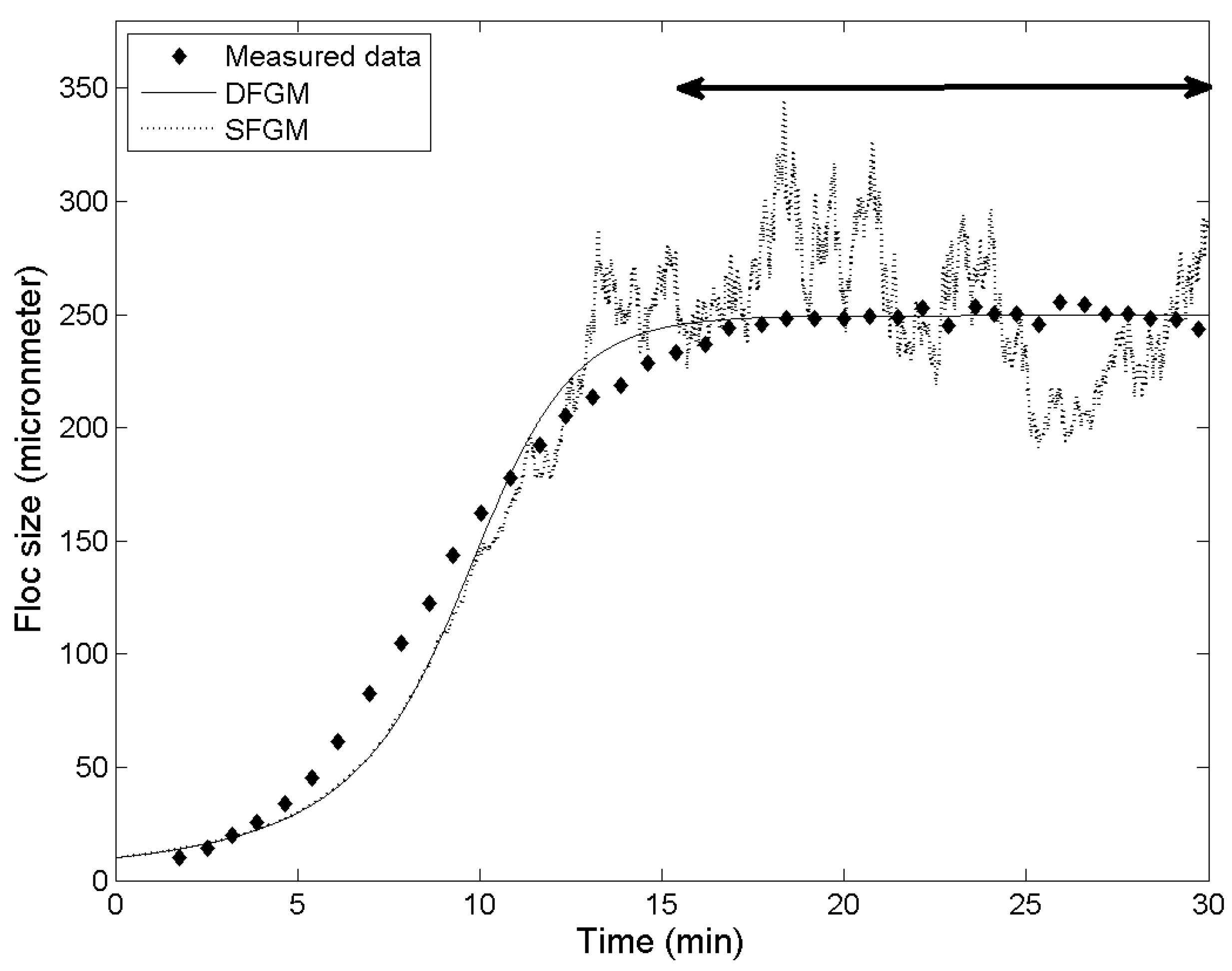
During each case of the experiment, 30 numerical simulations were conducted. This study focuses on the distribution of floc size in the equilibrium state. Therefore, the values of floc size at the last 1000 time steps (2061 total) are analyzed under the assumption that the flocculation process approaches a dynamic equilibrium state prior to 1061 time steps (see Figure 1). The stochastic FGM of this study is validated with 3 laboratory experiments by [9,23,24]. Following Spicer et al. [23], polystyrene particles were mixed in a stirred tank with an impeller in order to measure the size distribution of aggregates with volumetric and mass concentrations ( and c) of and 0.0147 kg/m3, respectively. The average value of G produced by the impeller is 50 s−1. The size and density of polystyrene particles (c and ) of the experiment are 0.87 μm and 1050 kg/m3, respectively. In Biggs and Lant [9], the size distribution of activated sludge is reported under the experimental condition of G = 19.4 s−1 and = 0.05. Under the assumption that is 2650 kg/m3 and the density of sludge is 1300 kg/m3, the mass concentration is calculated to be 24.19 kg/m3. The activated sludge is mixed in a baffled batch vessel using a flat six-blade impeller. Burban et al. [24] also report the results of laboratory experiments with Detroit River sediment. c and G of the experiment are 0.8 kg/m3 and 200 s−1, respectively. d and of Detroit River sediment are assumed to be 4 μm and 2650 kg/m3 due to absence of further information. The detailed conditions of experiments are summarized in Table 1. The calibrated values of empirical coefficients are shown in Table 2.
Figure 1.
Example of numerical simulation and analysis data. Dots represent the experimental result of Spicer et al. [23]. Solid and dotted lines are the stochastic FGM (SFGM) of this study and the deterministic FGM (DFGM), respectively.
Figure 1.
Example of numerical simulation and analysis data. Dots represent the experimental result of Spicer et al. [23]. Solid and dotted lines are the stochastic FGM (SFGM) of this study and the deterministic FGM (DFGM), respectively.


| Experiment | c (kg/m3) | (kg/m3) | d (μm) | G (s−1) | |
|---|---|---|---|---|---|
| Spicer et al., (1998) | 0.0147 | 1050 | 0.87 | 50.0 | |
| Biggs and Lant (2000) | 0.05 | 24.19 (Assumed) | 2650 (Assumed) | 4.00 (Assumed) | 19.4 |
| Burban et al., (1989) | N.A. | 0.05 | 2650 (Assumed) | 4.00 (Assumed) | 200.0 |
Note: N.A.—Not available.
| Experiment | B1 | |||
|---|---|---|---|---|
| Spicer et al., (1998) | 6.74 | |||
| Biggs and Lant (2000) | 0.02 | |||
| Burban et al., (1989) | 0.30 |
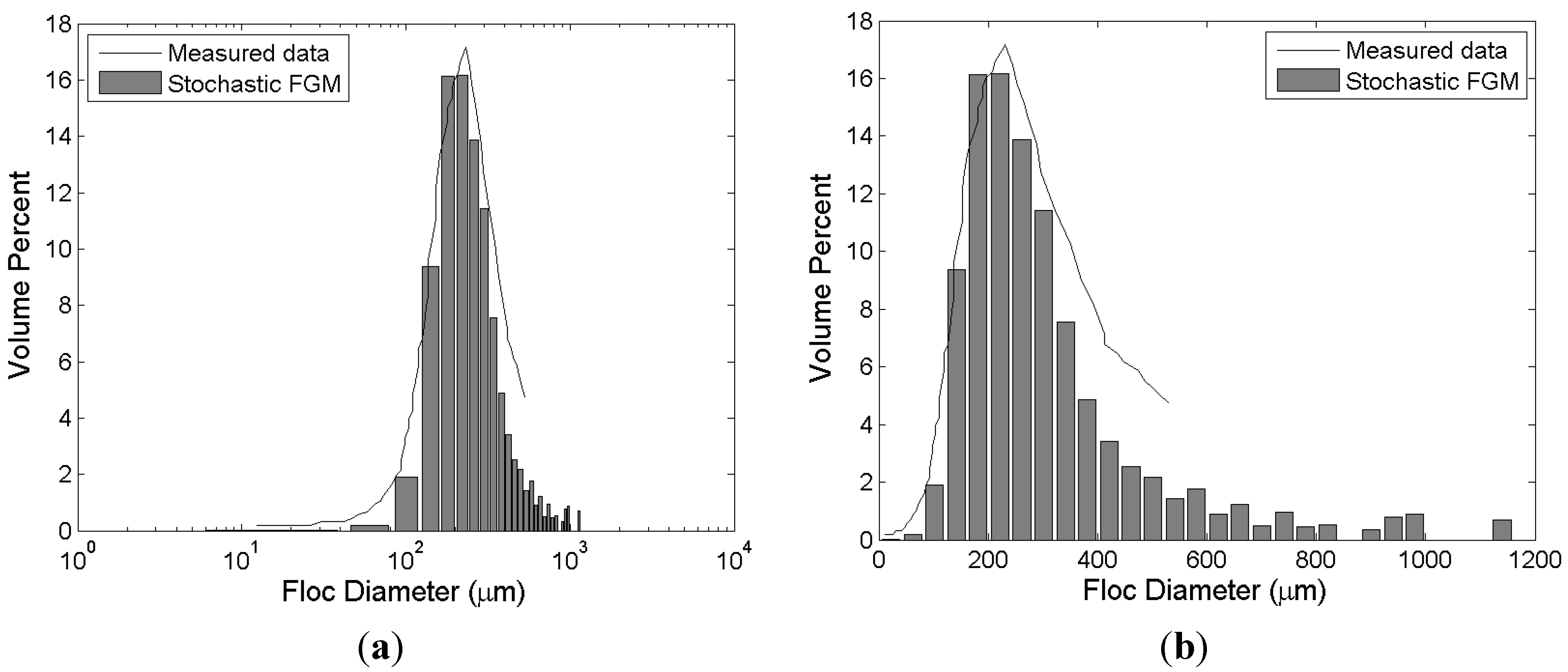
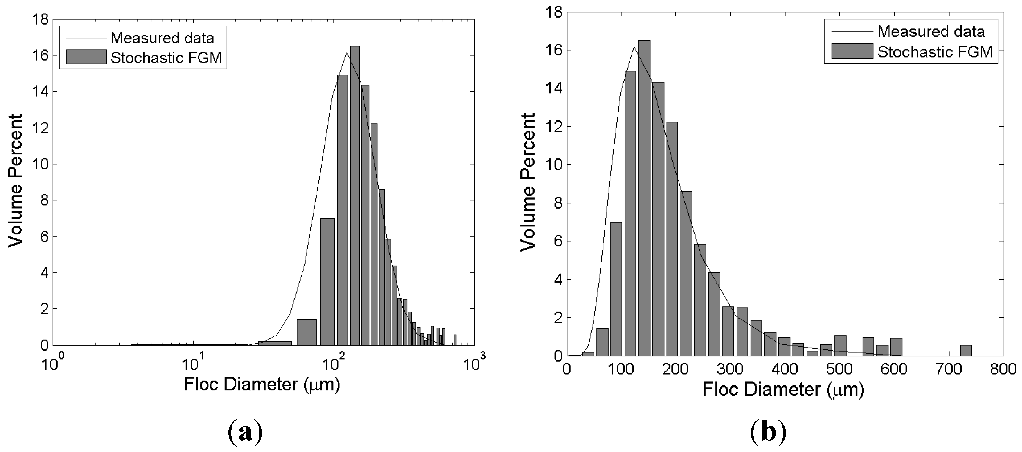
Figure 2 shows the simulation results of the stochastic FGM. The experiment from Spicer et al. [23] was carried out under the dilute condition (c = 0.0147 kg/m3). The intensity of turbulent shear is not low (G = 50 s−1). However, the mean size of flocs is about 200 μm. Therefore, it is clear that the polystyrene particles are easily aggregated. Under this assumption, the coefficient determining the aggregation efficiency has a relatively high value (). In terms of the mean size of flocs, the simulation results are in satisfactory agreement with experimental results. The mean size is determined by calibrating and . That is, the model has the capability to calculate mean size of flocs reasonably well. It is shown in Figure 2 that the calculated size distribution is positively skewed slightly more than the measured result. The log-normal distribution function has only 2 parameters, the mean and variance. Therefore, the skewness and kurtosis of log-normal distribution is indirectly determined by the values of mean and variance. Three- or four-parameter distribution functions such as generalized extreme value distribution and Wakeby distribution have the capability to determine the skewness or kurtosis by calibrating additional parameters. However, more empirical and site-specific parameters need to be calibrated when a 3- or 4-parameter distribution function is incorporated into FGM.
Figure 2.
Simulation results of stochastic FGM and experimental results of Spicer et al. [23]. The bars and the solid lines represent the experimental and simulation results, respectively. (a) semi-log axis; (b) normal (Cartesian) axis.
Figure 2.
Simulation results of stochastic FGM and experimental results of Spicer et al. [23]. The bars and the solid lines represent the experimental and simulation results, respectively. (a) semi-log axis; (b) normal (Cartesian) axis.

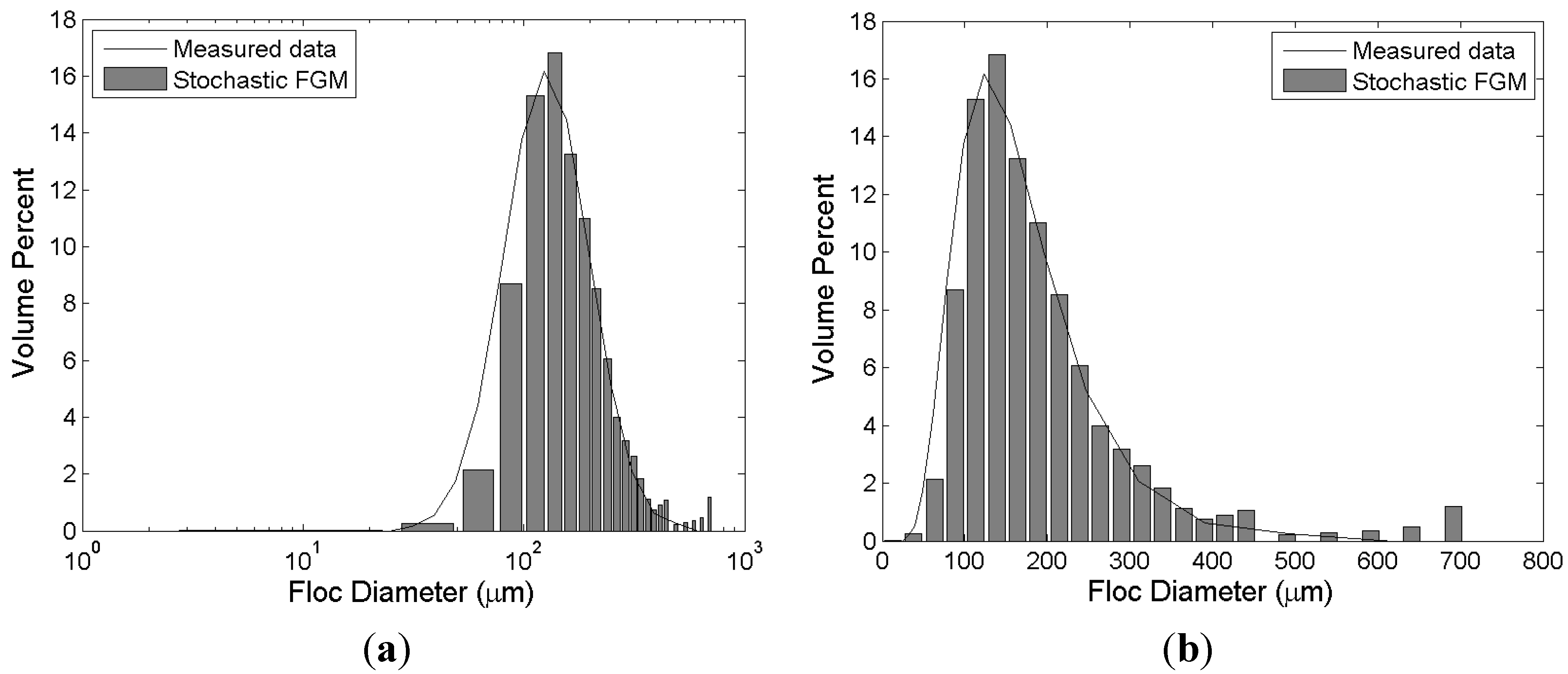
Figure 3 represents the results of stochastic simulation and measured data from Biggs and Lant [9]. Their experiment was conducted under conditions with very high concentration (c = 24.19 kg/m3). The intensity of turbulence is relatively low (G = 19.4 s−1). Under these conditions, the mean size of flocs is not large (about 120 μm). Therefore, it is deduced that the aggregation process of activated sludge used for the experiment has a low efficiency resulting in a low value for the aggregation efficiency parameter (). The simulation result is in a good agreement with laboratory measurements. Both the mean size and the distribution are reasonably replicated by the proposed stochastic FGM. The sudden increase of volume fraction around floc size 700 μm is due to the random property of stochastic simulation. Figure 4a shows the mean, maximum, and minimum floc sizes of 30 simulation cases. The dotted line is the equilibrium floc size calculated by the deterministic Son and Hsu FGM [1]. Figure 4b shows the temporal evolution of mean floc size measured by Biggs and Lant [9], a simulation result of deterministic FGM ([1]), and one case of simulation by stochastic FGM. As mentioned in the first paragraph of this section, the last 1000 values of floc size for each stochastic simulation are analyzed in this study. Therefore, the size distribution of this study is determined using 30,000 values for floc size. Figure 4 shows that a stochastic FGM calculates the floc size very randomly after the temporal evolution of floc size approaches the equilibrium state (around 15 min in Figure 4b). The maximum floc size among the values in the last 1000 time steps has a wide range (200 μm to 700 μm). Furthermore, the minimum floc size is also in the range of 10 μm to 50 μm whereas the mean values are between 70 and 120 μm in most cases.
Figure 3.
Simulation results of stochastic FGM and experimental results of Biggs and Lant [9]. The bars and the solid lines represent the experimental and simulation results, respectively. (a) semi-log axis; (b) normal (Cartesian) axis.
Figure 3.
Simulation results of stochastic FGM and experimental results of Biggs and Lant [9]. The bars and the solid lines represent the experimental and simulation results, respectively. (a) semi-log axis; (b) normal (Cartesian) axis.
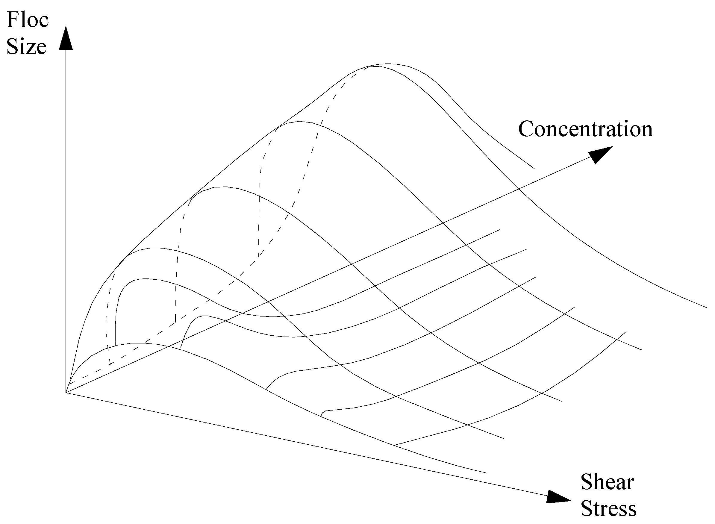
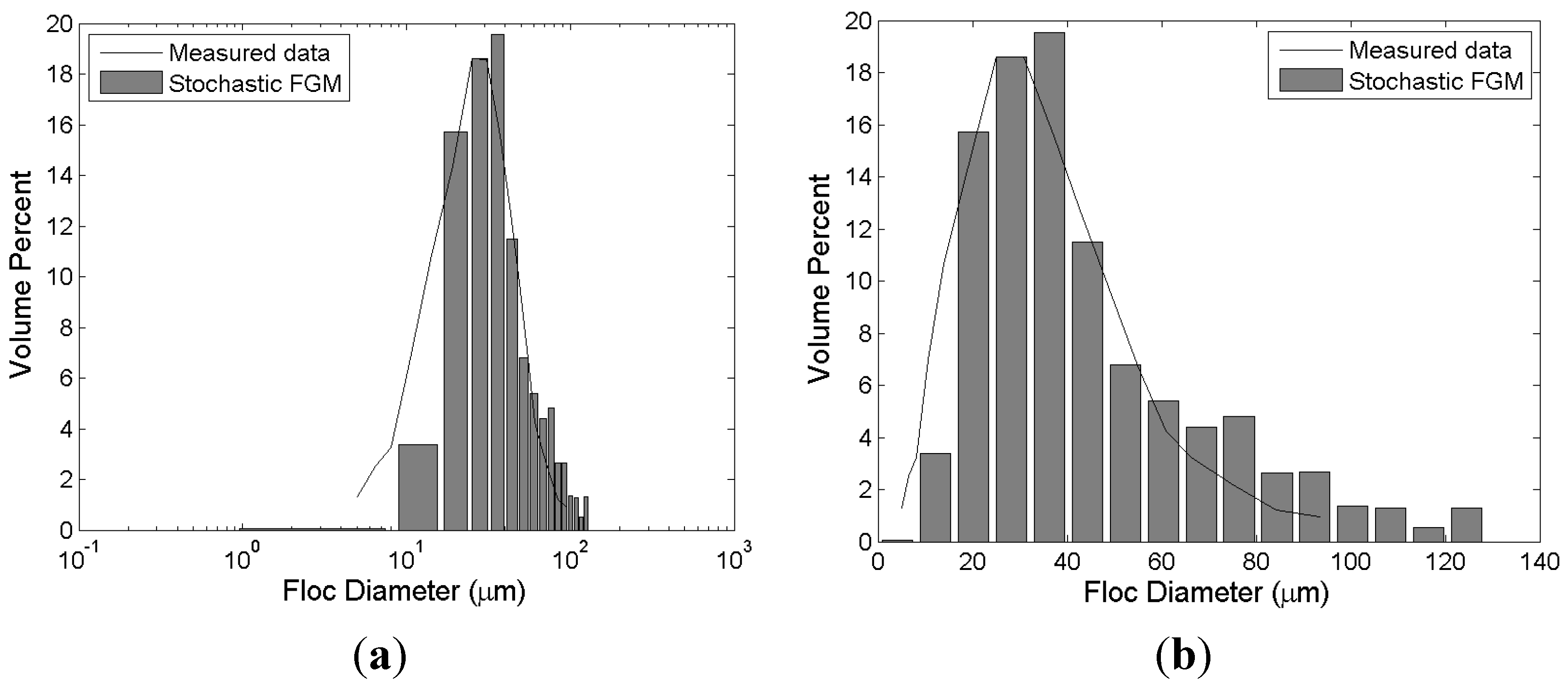
Burban et al. [24] measured the size distribution of Detroit River sediments with a high dissipation parameter (G = 200 s−1) and a moderate mass concentration condition (c = 0.8 kg/m3). Due to the high turbulence intensity, a high breakup efficiency is expected. Thus, the mean of is calibrated to be relatively high (μl = 3.95 × 10⁻⁵) compared to the two previous cases ([9,23]). Turbulent shear plays two conflicting and simultaneous roles in the flocculation process. The first one is to increase the chance of particle collisions resulting in floc aggregation. Turbulence is the most important mechanism of aggregation ([6,33,50,51]). The second role is disaggregation of flocs. Based on laboratory experiments, Tsai and Hwang [38] insist that a floc usually disaggregates into two roughly equal-sized daughter flocs. From this finding, it is deduced that the main mechanism of breakup is turbulent shear rather than particle collision. Figure 5 shows the effects of concentration and turbulent shear on mean floc size. Figure 5 shows that the high turbulent shear enhances the breakup process compared to aggregation process causing reduction of floc size ([2]). Therefore, the mean floc size of Burban et al. [24] is relatively small (about 20 μm) resulting in a high value for . Figure 6 shows the results of numerical simulation by stochastic FGM and measurements from Burban et al. [24]. The volume fraction near the mean value is slightly overestimated by the stochastic FGM. However, the overall shape of the distribution is in good agreement with measurement results. The volume fraction slightly increases around floc size 80 μm due to the random nature of the stochastic model. A stochastic model is usually based on a random number generation technique (pseudorandom number generator in this study). Therefore, perturbations due to randomness are inevitable.
Figure 4.
The random calculation of stochastic FGM. The dotted line of (a) shows the simulation results of deterministic FGM (DFGM). The circle, square, and triangle symbols represent the maximum, mean, and minimum values of each simulation, respectively; the solid and dotted lines of (b) are the results of deterministic FGM (DFGM) and stochastic FGM (SFGM), respectively; (a) mean, maximum, and minimum floc size (b) temporal evolution of floc size.

Figure 5.
Conceptual diagram representing effect of turbulent shear on mean floc size.

Figure 6.
Simulation results of stochastic FGM and experimental results of Burban et al. [24]. The bars and the solid lines represent the experimental and simulation results, respectively. (a) semi-log axis; (b) normal (Cartesian) axis.
Figure 6.
Simulation results of stochastic FGM and experimental results of Burban et al. [24]. The bars and the solid lines represent the experimental and simulation results, respectively. (a) semi-log axis; (b) normal (Cartesian) axis.

Three more probability distributions have been tested. The results of stochastic FGM using a normal distribution are drawn in Figure 7. The results are compared with Biggs and Lant [9]. A normal distribution has two parameters: mean and variance. The values of mean and variance of normal distribution are calibrated to be 2.620 × 10−5.0 and 5.623 × 10−5.0, respectively. Figure 8 shows the result of stochastic FGM using a Pearson type 3 distribution (Gamma distribution). A Pearson type 3 distribution needs 2 parameters: shape parameter (kp) and scale parameter (θ). The mean and variance of Pearson type 3 distributions are indirectly determined by kpθ and kpθ2, respectively. Therefore, it is not simple to calibrate a stochastic FGM. The determined values of kp and θ for the simulation are 4.780 × 10−1.0 and, 5.248 × 10−5.0, respectively. Compared to results of the log-normal distribution (Figure 3), FGMs using a normal distribution and a Pearson type 3 distribution overestimate the mean floc size, whereas the overall shape of size distribution is underestimated. Figure 9 represents the results calculated by stochastic FGM using a generalized extreme value (GEV) distribution. A GEV distribution has 3 parameters: mean, variance, and shape parameter (). In this study, the mean, variance, and
of the GEV distribution are set to be 1.147 × 10−5.0, 1.0 × 10−5.0 and 0.5, respectively. In the case of the GEV distribution, the floc size larger than the mean value is overestimated. Although a GEV distribution has one more degree of freedom () compared to log-normal distribution, no significant advantage is found.
4. Conclusions
This paper presents a stochastic FGM to calculate the size distribution of flocs. A stochastic approach is applied to the breakup process under the assumption that the aggregation process is significantly affected by properties of the sediment and carrier flow. For the stochastic approach, the parameter related to the breakup efficiency () is empirically assumed to have a log-normal distribution. From many previous studies under low organic content conditions (e.g., [15,35,36,37]), it is known that the size distribution of flocs is similar to a log-normal distribution. The capacity and limitations of the developed stochastic models are validated with three experimental results from Spicer et al. [23], Biggs and Lant [9], and Burban et al. [24]. These three experiments have different experimental conditions such as sediment property, turbulence intensity, and concentration.
Figure 7.
Simulation result of stochastic FGM using a normal distribution (compared to the experimental results of Biggs and Lant [9]). The bars and the solid lines represent the experimental and simulation results, respectively. (a) semi-log axis; (b) normal axis.
Figure 7.
Simulation result of stochastic FGM using a normal distribution (compared to the experimental results of Biggs and Lant [9]). The bars and the solid lines represent the experimental and simulation results, respectively. (a) semi-log axis; (b) normal axis.
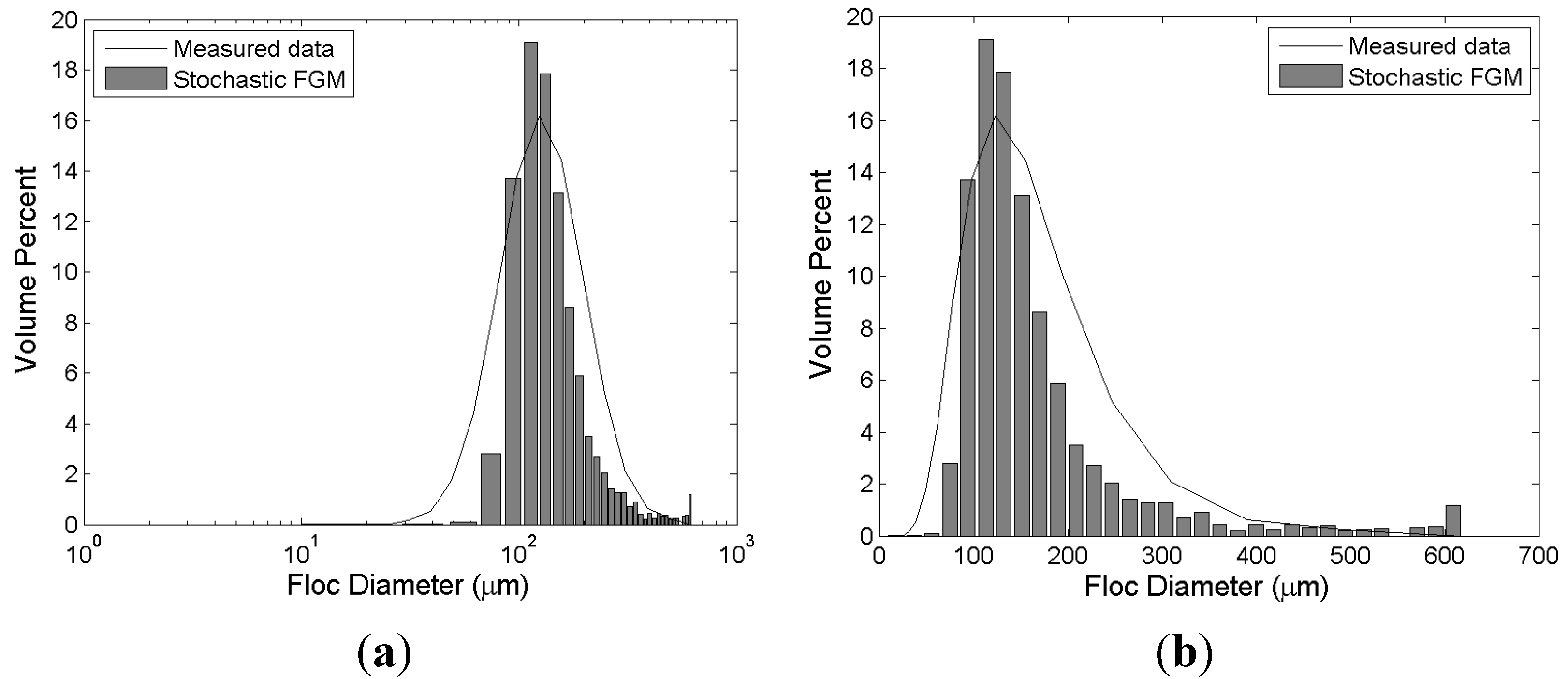
Figure 8.
Simulation result of stochastic FGM using a Pearson type 3 distribution (compared to the experimental results of Biggs and Lant [9]). The bars and the solid lines represent the experimental and simulation results, respectively. (a) semi-log axis; (b) normal (Cartesian) axis.
Figure 8.
Simulation result of stochastic FGM using a Pearson type 3 distribution (compared to the experimental results of Biggs and Lant [9]). The bars and the solid lines represent the experimental and simulation results, respectively. (a) semi-log axis; (b) normal (Cartesian) axis.

As examined in Section 3, a stochastic FGM using a log-normal distribution has the capability to replicate the size distribution of flocs to a reasonable extent. Three different probability distributions such as normal, Pearson type 3, and GEV distributions are also tested in this study. Among them, an FGM using a log-normal distribution has the advantage of accuracy and simplicity. When a normal distribution is applied, a stochastic FGM underestimates the distribution of flocs larger than 200 μm, although the variance and mode are calculated in conformity. This finding shows that the positive skewness of is needed to calculate large flocs reasonably well. The positive skewness of decreases the breakup possibility for relatively large flocs. Flocs become less dense and more fragile as the size of floc increases. As a result, large flocs have higher possibility of breakup. A stochastic FGM using a Pearson type 3 distribution shows a mean-concentrated distribution of floc size. The skewness of a Pearson type 3 distribution is inversely proportional to the shape parameter () whereas the variance is proportional to the shape parameter (). Therefore, the variance decreases resulting in the mean-concentrated distribution when the skewness is increased. The result of a GEV distribution is in good agreement with measurement results. Compared to a log-normal distribution, a GEV distribution has one more degree of freedom as mentioned in Section 3. Thus, the calibration of a GEV distribution is not found to be complicated relative to a log-normal distribution.
Figure 9.
Simulation result of stochastic FGM using a generalized extreme value distribution (compared to the experimental results of Biggs and Lant [9]). The bars and the solid lines represent the experimental and simulation results, respectively. (a) semi-log axis; (b) normal (Cartesian) axis.
Figure 9.
Simulation result of stochastic FGM using a generalized extreme value distribution (compared to the experimental results of Biggs and Lant [9]). The bars and the solid lines represent the experimental and simulation results, respectively. (a) semi-log axis; (b) normal (Cartesian) axis.

An FGM has an advantage in the sense that it ensures mass conservation in a closed system and can be easily incorporated into the numerical sediment transport model. The previous FGMs, such as those used by Son and Hsu [7] and Winterwerp [8], calculate the average size of flocs (representative floc size). Therefore, the sediment transport model considering the flocculation process also assumes the suspension of mono-sized sediment (e.g., [25]). When a stochastic FGM discussed in this study is incorporated with the sediment transport model, it has the capability to calculate the size distributions of suspended cohesive sediments (flocs) as well as the temporal and spatial variation of floc concentration. Hence, future incorporation of these results (i.e., stochastic FGMs) to sediment transport models will greatly improve resolution and uncertainty, furthering our knowledge of cohesive sediment transport processes.
In this study, the mean of ( in Equation (3)) is assumed to be constant following the previous studies (e.g., [1,7,8]). is a parameter representing the probability of floc breakup. As the size of floc increases, the probability of breakup is also expected to increase because the yield stress of floc usually depends on floc size. Therefore, it is necessary to study the effect of floc size evolution through the flocculation process on calibration of in the future. It is also notable that the time step size may affect the calculation of floc size distribution. In this study, the time step for the numerical calculation is automatically determined by the Dormand-Prince method. In order to examine the effect of the time step, it is necessary to calculate the stochastic FGM with different fixed time step values.
Acknowledgments
This research was supported by the Basic Science Research Program through the National Research Foundation of Korea (NRF) funded by the Ministry of Education, Science and Technology (2011-0010749), the research fund of Chungnam National University in 2014, and a project, “Development of integrated estuarine management system”, funded by the Ministry of Oceans and Fisheries of Korea.
Author Contributions
H. J. Shin and M. Son conceived the experiments; M. Son wrote the paper; H. J. Shin performed the experiments; H. J. Shin and G. Lee analyzed the results.
Conflicts of Interest
The authors declare no conflict of interest.
References
- Son, M.; Hsu, T.-J. The effect of variable yield strength and variable fractal dimension on flocculation of cohesive sediment. Water Res. 2009, 43, 3585–3592. [Google Scholar]
- Dyer, K.R. Sediment processes in estuaries: Future research requirements. J. Geophys. Res. 1989, 94, 14327–14339. [Google Scholar] [CrossRef]
- Dyer, K.R.; Manning, A.J. Observation of the size, settling velocity and effective density of flocs, and their fractal dimensions. J. Sea Res. 1999, 41, 87–95. [Google Scholar] [CrossRef]
- Lick, W.; Lick, J.; Ziegler, C.K. Flocculation and its effect on the vertical transport of fine-grained sediments. In Sed./Water Interactions, Hydrobiologia; Hart, B.T., Sly, P.G., Eds.; Kluwer Academic Publishers: Dordrecht, The Netherlands, 1992; pp. 1–16. [Google Scholar]
- Hunt, J.R. Particle dynamics in seawater: Implications for predicting the fate of discharged particles. Environ. Sci. Tech. 1982, 16, 303–309. [Google Scholar] [CrossRef]
- Stolzenbach, K.D.; Elimelich, M. The effect of density on collisions between sinking particles: Implications for particle aggregation in the ocean. Deep Sea Res. Part I: Oceanogr. Res. Pap. 1994, 41, 469–483. [Google Scholar]
- Son, M.; Hsu, T.-J. Flocculation model of cohesive sediment using variable fractal dimension. Environ. Fluid Mech. 2008, 8, 55–71. [Google Scholar] [CrossRef]
- Winterwerp, J.C. A simple model for turbulence induced flocculation of cohesive sediment. J. Hydraul. Res. 1998, 36, 309–326. [Google Scholar] [CrossRef]
- Biggs, C.A.; Lant, P.A. Activated sludge flocculation: On-line determination of floc size and the effect of shear. Water Res. 2000, 34, 2542–2550. [Google Scholar] [CrossRef]
- Bouyer, D.; Line, A.; Do-quang, Z. Experimental analysis of floc size distribution under different hydrodynamics in a mixing tank. AIChE 2004, 50, 2064–2081. [Google Scholar] [CrossRef]
- Tsai, C.H.; Hwang, S.C. Flocculation of sediment from the Tanshui River estuary. Mar. Freshw. Res. 1995, 46, 383–392. [Google Scholar]
- Tsai, C.H.; Iacobellis, H.S.; Lick, W. Flocculation of fine-grained sediments due to a uniform shear stress. J. Great Lakes Res. 1987, 13, 135–146. [Google Scholar] [CrossRef]
- Maggi, F.; Mietta, F.; Winterwer, J.C. Effect of variable fractal dimension on the floc size distribution suspended cohesive sediment. J. Hydrol. 2007, 343, 43–55. [Google Scholar] [CrossRef]
- McAnally, W.H.; Mehta, A.J. Aggregation rate of fine sediment. J. Hydraul. Eng. 2000, 126, 883–892. [Google Scholar] [CrossRef]
- Verney, R.; Lafite, R.; Brun-Cottan, J.C.; le Hir, P. Behaviour of floc population during a tidal cycle: Laboratory experiments and numerical modeling. Cont. Shelf Res. 2011. [Google Scholar] [CrossRef]
- Lick, W.; Huang, H.; Jepsen, R. Flocculation of fine-grained sediments due to differential settling. J. Geophys. Res. 1993, 98, 10279–10288. [Google Scholar] [CrossRef]
- Hounslow, M.J.; Ryall, R.L.; Marshall, V.R. A discretized population balance for nucleation, growth and aggregation. AIChE 1988, 34, 1821–1832. [Google Scholar] [CrossRef]
- Maerz, J.; Verney, R.; Wirtz, K.; Feudel, U. Modeling flocculation processes: Intercomparison of a size class-based model and a distribution-based model. Continental Shelf Res. 2011. [Google Scholar] [CrossRef]
- Levich, V.G. Physicochemical Hydrodynamics; Prentice Hall: Upper Saddle River, NJ, USA, 1962. [Google Scholar]
- Khelifa, A.; Hill, P.S. Models for effective density and settling velocity of flocs. J. Hydraul. Res. 2006, 44, 390–401. [Google Scholar] [CrossRef]
- Maggi, F. Variable fractal dimension: A major control for floc structure and flocculation kinematics of suspended cohesive sediment. J. Geophys. Res. 2007, 112. [Google Scholar] [CrossRef]
- Sonntag, R.C.; Russel, W.B. Structure and breakup of flocs subjected to fluid stresses. II. Theory. J. Colloid Interface Sci. 1987, 115, 378–389. [Google Scholar] [CrossRef]
- Spicer, P.T.; Pratsinis, S.E.; Raper, J.; Amal, R.; Bushell, G.; Meesters, G. Effect of shear schedule on particle size, density, and structure during flocculation in stirred tanks. Power Tech. 1998, 97, 26–34. [Google Scholar] [CrossRef]
- Burban, P.Y.; Lick, W.; Lick, J. The flocculation of fine-grained sediments in estuarine waters. J. Geophys. Res. 1989, 94, 8323–8330. [Google Scholar] [CrossRef]
- Son, M.; Hsu, T.-J. The effects of flocculation and bed erodibility on modeling cohesive sediment resuspension. J. Geophys. Res. 2011, 116. [Google Scholar] [CrossRef]
- Van der Ham, R.; Fontijn, R.H.L.; Kranenburg, C.; Winterwerp, J.C. Turbulent exchange of fine sediments in a tidal channel in the Ems/Dollard estuary. Part I: Turbulence measurement. Cont. Shelf Res. 1994, 21, 1605–1628. [Google Scholar] [CrossRef]
- Son, M.; Lee, G.-H. On effects of skewed and asymmetric oscillatory flows on cohesive sediment flux: Numerical study. Water Resources Res. 2013, 49, 4409–4423. [Google Scholar] [CrossRef]
- Man, C.; Tsai, C.W. Stochastic partial differential equation-based model for suspended sediment transport in surface water flow. J. Eng. Mech. 2007, 133, 422–430. [Google Scholar] [CrossRef]
- Davie, A.M.; Gaines, J.G. Convergence of numerical schemes for the solution of parabolic stochastic partial differential equations. Math. Comput. 1999, 70, 121–134. [Google Scholar] [CrossRef]
- Gyongy, I. Lattice approximation for stochastic quasi-linear parabolic partial differential equations driven by space-time white noise II. Potential Anal. 1999, 11, 1–37. [Google Scholar] [CrossRef]
- Yoo, H. Semi-discretization of stochastic partial differential equations on R1 by a finite-difference method. Math. Comput. 2000, 69, 653–666. [Google Scholar] [CrossRef]
- Maggi, F. Stochastic flocculation of cohesive sediment: Analysis of floc mobility within the floc size spectrum. Water Resour. Res. 2008, 44. [Google Scholar] [CrossRef]
- McCave, I.N. Size spectra and aggregation of suspended particles in the deep ocean. Deep Sea Res. 1984, 31, 329–352. [Google Scholar] [CrossRef]
- Hill, P.S.; Boss, E.; Newgard, J.P.; Law, B.A.; Milligan, T.G. Observations of the sensitivity of beam attenuation to particle size in a coastal bottom boundary layer. J. Geophys. Res. 2011, 116, C02023. [Google Scholar]
- Mikkelsen, O.A.; Milligan, T.G.; Hill, P.S.; Moffatt, D. INSSECT–and instrumented platform for investigating floc properties close to the seabed. Limnol. Oceanogr. Methods 2004, 2, 226–236. [Google Scholar] [CrossRef]
- Mikkelsen, O.A.; Hill, P.S.; Milligan, T.G.; Chant, R.J. In situ particle size distributions and volume concentrations from a LISST-100 laser particle sizer and a digital floc camera. Cont. Shelf Res. 2005, 25, 1959–1978. [Google Scholar] [CrossRef]
- Mikkelsen, O.A.; Hill, P.S.; Milligan, T.G. Single-grain, microfloc and macrofloc volume variations observed with a LISST-100 and a digital floc camera. J. Sea Res. 2006, 55, 87–102. [Google Scholar] [CrossRef]
- Syvitski, J.P.M.; Hutton, E.W.H. In situ charateristics of suspended particles as determined by the floc camera assembly FCA. J. Sea Res. 1996, 36, 131–142. [Google Scholar] [CrossRef]
- Xu, F.; Wang, D.-P.; Riemer, N. Modeling flocculation processes of fine-grained particles using a size-resolved method: Comparison with published laboratory experiments. Cont. Shelf Res. 2008, 28, 2668–2677. [Google Scholar] [CrossRef]
- Manning, A.J. Observation of the properties of flocculated cohesive sediment in three western European estuaries. J. Coastal Res. 2002, SI 41, 70–81. [Google Scholar]
- Manning, A.J.; Dyer, K.R.; Lafite, R.; Mikes, D. Flocculation measured by video based instruments in the Gironde estuary during the European Commission SWAMIEE Project. J. Coastal Res. 2004, SI 41, 58–69. [Google Scholar]
- Manning, A.J.; Bass, S.J.; Dyer, K.R. Observations of cohesive sediment settling fluxes in high energy tidal estuarine environments. Mar. Geol. 2006, 235, 177–192. [Google Scholar] [CrossRef]
- Manning, A.J.; Friend, P.L.; Prowse, N.; Amos, C.L. Estuarine mud flocculation properties determined using an annular mini-flume and the LabSFLOC system. Cont. Shelf Res. 2007, 27, 1080–1095. [Google Scholar] [CrossRef]
- Gratiot, N.; Manning, A.J. An experimental investigation of floc characteristics in a diffusive turbulent flow. J. Coast. Res. 2004, SI 41, 105–113. [Google Scholar]
- Gibbs, R.J. Coagulation rates of clay minerals and natural sediment. J. Sediment Res. 1983, 53, 1193–1203. [Google Scholar]
- Lick, W.; Lick, J. Aggregation and disaggregation of fine-grained sediments. J. Great Lakes Res. 1988, 14, 514–523. [Google Scholar] [CrossRef]
- Mietta, F. Evolution of the Floc Size Distribution of Cohesive Sediments. Ph.D. Thesis, Delft University, Delft, The Netherlands, 2010. [Google Scholar]
- Maggi, F. Flocculation Dynamics of Cohesive Sediment. Ph.D. Thesis, Delft University, Delft, The Netherlands, 2005. [Google Scholar]
- Serra, T.; Casamitjana, X. Effect of the shear and volume fraction on the aggregation and break-up of particle. Am. Instit. Chem. Eng. 1998, 44, 1724–1730. [Google Scholar] [CrossRef]
- O’Melia, C.R. Aquasols: The behavior of small particles in aquatic systems. Env. Sci. Technol. 1980, 14, 1052–1060. [Google Scholar] [CrossRef]
- Van Leussen, W. Estuarine Macroflocs and Their Role in Fine-Grained Sediment Transport. Ph.D. Dissertation, University of Utrecht, Utrecht, The Netherlands, 1994. [Google Scholar]
© 2015 by the authors; licensee MDPI, Basel, Switzerland. This article is an open access article distributed under the terms and conditions of the Creative Commons Attribution license (http://creativecommons.org/licenses/by/4.0/).
Share and Cite
MDPI and ACS Style
Shin, H.J.; Son, M.; Lee, G.-h. Stochastic Flocculation Model for Cohesive Sediment Suspended in Water. Water 2015, 7, 2527-2541. https://doi.org/10.3390/w7052527
AMA Style
Shin HJ, Son M, Lee G-h. Stochastic Flocculation Model for Cohesive Sediment Suspended in Water. Water. 2015; 7(5):2527-2541. https://doi.org/10.3390/w7052527
Chicago/Turabian StyleShin, Hyun Jung, Minwoo Son, and Guan-hong Lee. 2015. "Stochastic Flocculation Model for Cohesive Sediment Suspended in Water" Water 7, no. 5: 2527-2541. https://doi.org/10.3390/w7052527