Article

Assessing Potential Algal Blooms in a Shallow Fluvial Lake by Combining Hydrodynamic Modelling and Remote-Sensed Images

1
Institute for Electromagnetic Sensing of the Environment, National Research Council, Via Bassini 15, Milan 20133, Italy
2
Department of Life Sciences, University of Parma, Viale Usberti 11/a, Parma 43124, Italy
3
Department of Civil Engineering and Architecture, University of Pavia, Via Ferrata 3, Pavia 27100, Italy
*
Author to whom correspondence should be addressed.
Water 2015, 7(5), 1921-1942; https://doi.org/10.3390/w7051921
Submission received: 2 February 2015 / Revised: 11 April 2015 / Accepted: 24 April 2015 / Published: 28 April 2015
(This article belongs to the Special Issue Water Quality Control and Management)

Abstract

:
Shallow fluvial lakes are dynamic ecosystems shaped by physical and biological factors and characterized by the coexistence of phytoplankton and macrophytes. Due to multiple interplaying factors, understanding the distribution of phytoplankton in fluvial lakes is a complex but fundamental issue, in the context of increasing eutrophication, climate change, and multiple water uses. We analyze the distribution of phytoplankton by combining remotely sensed maps of chlorophyll-a with a hydrodynamic model in a dammed fluvial lake (Mantua Superior Lake, Northern Italy). The numerical simulation of different conditions shows that the main hydrodynamic effects which influence algal distribution are related to the combined effect of advection due to wind forces and local currents, as well as to the presence of large gyres which induce recirculation and stagnation regions, favoring phytoplankton accumulation. Therefore, the general characters of the phytoplankton horizontal patchiness can be inferred from the results of the hydrodynamic model. Conversely, hyperspectral remote-sensing products can be used to validate this model, as they provide chlorophyll-a distribution maps. The integration of ecological, hydraulic, and remote-sensing techniques may therefore help the monitoring and protection of inland water quality, with important improvements in management actions by policy makers.

1. Introduction

Fluvial lakes are, in general, highly dynamic shallow water bodies where different communities of primary producers coexist and are shaped by an array of physical and biological factors. They may undergo large interannual variations of residence time, depending upon water discharge, which is in turn related to rainfall patterns and water diversion for human activities. Fluvial lakes may also display fluctuating concentrations of inorganic nutrients and chlorophyll-a (a proxy of algal biomass), depending upon the rates of primary production and of microbial activity. Hydrological alterations (e.g., river damming, water diversion) intensify the effect of high nutrient loading from upstream: a decrease in water discharge has consequences on water renewal, thermal stratification, primary producer communities and photosynthetic rates [1], gas and nutrient dynamics [2], and benthic processes [3]. Fluvial lakes may also host dense stands of different groups of submersed, floating leaved or emergent macrophytes, each locally affecting water circulation and biogeochemical processes.
As a consequence of multiple interplaying factors, the distribution of phytoplankton in fluvial lakes is a complex issue. The capacity to predict pelagic algae distribution and abundance is, however, important in the context of increasing eutrophication, unpredictable climate, and multiple water use. The general variability of phytoplankton communities is influenced both by physical factors, such as variable wind patterns, discharge and light availability [4] and by biological processes, such as the presence of macrophyte islands and the interaction between benthic and pelagic compartments (e.g., hypoxia or anoxia events and coupled nutrient dynamics) [5,6].
According to Verhagen [7], a likely time scale for algal growth and decay is ~10 d. Therefore, having the usual advection time scales in the order of a few hours [8,9,10,11], phytoplankton can be assumed to be passively transported, except for very large shallow lakes. Time scales for phytoplankton horizontal distribution can then be assimilated to the ones of lake circulations. Thus, in shallow fluvial lakes, wind and discharge, in addition to shaping hydrodynamics, play also a major role in determining the large-scale distribution of phytoplankton and passively-advected zooplankton [8,12,13]. Microorganism arrangement is also the vector through which hydrodynamically induced patchiness is transferred to higher trophic levels [14]. Biological processes are hence relevant only over multi-daily time scales or over very small spatial scales [15].
Circulation patterns in shallow lakes can be divided into two categories [16]: “conveyor belt” type, in which prevailing circulations develop in the vertical plane, and “Livingstone-type” [17], in which water motions develop in the horizontal plane. George & Edwards [18] found that, in a lake with prevailing circulations in the vertical plane, organisms which tend to concentrate near the surface accumulate in downwelling regions downstream, while the ones which tend to aggregate near the bottom or the thermocline, hence are transported by return currents, accumulate in upwind upwelling regions. In such a situation, the horizontal distribution of plankton is linked to the vertical one [19]. According to the observations by George & Edwards [18] on a shallow reservoir with prevailing circulation in the vertical plane, cyanobacteria concentrate near the water surface because of their positive buoyancy, being mixed along the water depth by turbulence for wind speeds above 4 m/s. In this case, horizontal patchiness is observed only for low winds, as the return current homogenizes the distribution for higher intensities. For shallow lakes with Livingstone-type circulations, horizontal patchiness persists even for stronger winds, even if more mixed conditions are attained.
Located in Northern Italy, the Mantua Lakes system (Superior, Middle, and Inferior Lakes) is an interesting case study with respect to phytoplankton distribution and transport. These lakes are shallow, nutrient-enriched, host different primary producers, and undergo pronounced interannual discharge variations, coinciding with seasonal water diversion for irrigation purposes and rainfall patterns. The interaction between the continuous import of nutrients and export of particulate matter, the hydrological regime and the lake morphology leads to a mosaic of environmental conditions, allowing the simultaneous occurrence of different macrophyte typologies and high phytoplankton biomass [20]. Bolpagni et al. [21] found generally lower concentrations of chlorophyll-a (Chl-a) in the areas closest to the macrophyte stands compared to the outer zone and speculated allelopatic interactions or nutrient limitation. They did not include in their study water circulation, which in eutrophic fluvial lakes shapes the primary producer community [22,23,24,25].
Legendre and Demers [14] called the coupled study of biological and hydrodynamic processes “dynamic biological limnology”. In this frame, biological dynamics can be used to estimate hydrodynamic patterns e.g., [26]: for example, remote-sensed images of Chl-a distribution can be used to validate wind-induced circulation models [7], while numerical model results can be used to assess the correlation between plankton distribution and hydrodynamic variables [8]. Thackeray et al. [15] pointed out that given the responsive nature of plankton distribution to wind variations, the results of field surveys taking many hours or days to complete cannot describe properly the distribution dynamics. In this sense, remote-sensed images are the most appropriate tool, as they capture instantaneously the whole water body.
The full coupling between ecological and hydrodynamic models, with a large number of equations and calibration parameters for the ecological part e.g., [27,28], is an advancing field in limnology, leading to physically-based interpretations, replacing black-box approaches [29]. The use of coupled ecological and hydrodynamic models is justifiable over long time scales (e.g., seasonal and multi-annual) and very large spatial scales (e.g., very large lakes and sea areas) [30]. Under such circumstances, in fact, there is an interplay between physical and biological processes. This is not the case for shallow fluvial lakes, where phytoplankton horizontal patchiness is an almost exclusive product of hydrodynamic factors, so that its determination can be obtained on a hydrodynamic basis only.
The main objective of this work is the analysis of the distribution of phytoplankton in the Superior Lake of Mantua, through the comparison of remotely sensed maps of Chl-a, derived in previous studies [21,31,32] with the results of a newly-developed numerical hydrodynamic model, in order to identify the circulation patterns responsible for algal patchiness. Four historical situations were analyzed, including a dry summer case, characterized by extremely low flow and long water residence time. The consistent relations found between the hydrodynamic variables and phytoplankton distribution also provide an indirect validation of the numerical model.

2. Materials and Methods

2.1. Study Area

The Superior Lake of Mantua (surface area 3.67 km2, average depth 3.6 m) is the uppermost of three shallow hypertrophic fluvial lakes, located in a highly human-impacted (for agriculture and industrial purposes) sub-basin of the Po River in Northern Italy (Figure 1). The lakes system was created in the 12th century by the damming of the Mincio River. The water discharge in the Superior Lake of Mantua is regulated by the Vasarone sluice gate and by the recently-opened Vasarina gate, maintaining a constant water level of 17.5 m a.s.l. The average water residence time of the lake in the period 2000–2006 was ~8 days (mean discharge Q = 20 ± 6 m3 s−1). Some small secondary tributaries along the lake left shore also contribute to the discharge, with an overall mean summer inflow of about 5 m3 s−1, mainly due to the drainage from crop fields. The Mantua Lakes system has been part of the UNESCO World Cultural Heritage since 2008 and is protected as a Natural Regional Park. Moreover, the Superior Lake is located just downstream of the “Valli del Mincio” wetlands Natural Reserve, which is also a Site of Community Importance.
Figure 1. (a) Geographic position of the Mantua Lakes system; (b) Bathymetry of the Superior Lake of Mantua (ortophotos courtesy of Lombardy Region).
Water 07 01921 g001
The Superior Lake of Mantua receives high nutrient loads from the Mincio River, which sustain a high primary producer growth (0.1 mg/L N–NH4+, 2.1 mg/L N–NO3, 0.1 mg/L P–TP; average data by ARPA—Regional Environmental Protection Agency—Lombardy 2003–2011). In this fluvial lake, allochtonous nutrient loads, generated upstream, largely exceed those recycled (or retained/lost) from sediments [20]. The water transparency average value is 1.1 ± 0.6 m (variations mainly due to particulate matter and phytoplankton growth), while Chl-a concentrations vary between a few and ~200 mg m−3 (data source: ARPA Lombardy 2003–2011). Daylight oxygen saturation is, on average, above the equilibrium (137% ± 59%; data source: ARPA Lombardy 2003–2011).
Eutrophic to hypertrophic conditions result in dense phytoplankton communities, such as chlorophytes, euglenophytes, chrysophytes, diatoms and cyanophytes [4], that strongly limit available light to submersed macrophytes.
The shallower areas of the Superior Lake host different groups of macrophytes (emergent e.g., Phragmites australis, submersed e.g., Ceratophyllum demersum and floating-leaved e.g., Nelumbo nucifera). N. nucifera, the lotus flower, pervasively colonises an extensive area of the lake surface forming islands, the widest one being located in the south-eastern portion of the lake (Figure 1b).

2.2. Remote Sensing Data

Remotely sensed images used in this study were acquired from both satellite and airborne platforms and include data from three hyperspectral sensors. Airborne data were acquired by MIVIS (Multispectral Infrared Visible Imaging Spectrometer) and APEX (Airborne PRISM Experiment). These sensors operate with different technologies, as MIVIS is a whisk broom scanner, while APEX is a dispersive push broom imaging spectrometer. MIVIS measures the reflected radiation in 102 bands 0.441–12.42 μm, but the ones relevant for water quality studies are the first 20 nm wide 20 bands 0.441–0.820 μm. Within this spectral range, APEX has a finer spectral resolution, providing 98 bands 0.426–0.910 μm, with a bandwidth between 3.5 and 13 nm. The satellite images were acquired from CHRIS sensors (Compact High Resolution Imaging Spectrometer) onboard of PROBA (PRoject for On-Board Autonomy). CHRIS-PROBA is a physically compact payload, as its name implies (it weighs less than 15 kg), and operates in the push broom mode. CHRIS-PROBA images have 18 bands with a bandwidth between 12 and 20 nm, useful for water related applications [33].
The airborne campaigns with MIVIS and APEX were performed on 26 July 2007 and on 21 September 2011 and provided data with a spatial resolution of 4 m and 3 m, respectively.CHRIS-PROBA images at 18 m spatial resolution were acquired in between the two airborne campaigns, on 29 June 2008 and 28 August 2011. Land features and macrophyte-covered water regions were first masked out. Then, the four images were transformed into Chl-a concentration distribution maps as described in [4,21,31,32], having been first corrected for atmospheric effects and then converted to Chl-a concentration by semi-empirical approaches. These methods, which are widely used in productive waters to assess the Chl-a concentration, employ band ratios between the secondary Chl-a absorption maximum (~675 nm) and adjacent spectral bands not affected by phytoplankton absorption, such as the near-infrared reflectance peak near 700 nm e.g., [34]. The use of the band ratios to estimate Chl-a from remotely sensed images was evaluated by using field data collected at the time of imagery acquisitions. The average relative error for the three sensors was 20%. Due to water transparency being much smaller than the water depth, except immediately nearshore, the remotely sensed signal is essentially not affected by bottom reflection. Details on the transformation of images into Chl-a concentration maps are given in Table 1.

2.3. Numerical Hydrodynamic Lake Model

A 3D numerical model of the hydrodynamics of the Superior Lake of Mantua was developed, implementing the relevant physical phenomena that shape circulations. Topography was obtained by the Kriging interpolation of a low-resolution bathymetrical survey, integrated by a 2012 airborne image by the Lombardy Region for the definition of lake shores and lotus flower island borders (Figure 1b). Because of the limited data, the upstream boundary of the model was set at the entrance to the actual lacustrine part of the lake, leaving out the channelized transitional section from the ‘Valli del Mincio’ wetlands.
Table 1. List of algorithms with related accuracy (R2) used to transform remote-sensed reflectances (Rw) into chlorophyll-a (Chl-a) concentration maps. The rRMSE (relative Root Mean Square Error) gives the percentage error when the algorithms are applied to the images.
SensorDataAlgorithmR2rRMSE [%]References
APEX21 September 201154.647 × [Rw(690,697) − Rw(670,673)] − 52.470.8627[4,21]
CHRIS29 June 200881.257 × [Rw(706) − Rw(669)] – 54.50.7416[32]
MIVIS26 July 2007170.81 × [Rw(677) − Rw(710)] × Rw(747) + 36.1050.7718[31]
The general arrangement of circulations in the Superior Lake of Mantua is more of the “Livingstone-type” rather than the ‘conveyor belt’ type, due to the bathymetrical inhomogeneities (Figure 1b), the complex shape and the strong through-flowing current of the Mincio River: three-dimensional effects are present only locally. This leads to noticeable phytoplankton horizontal patchiness [7]. Levasseur et al. [35] observed that, in estuarine environments, stronger winds are needed to homogenize the horizontal distribution because of the strong tidal current: similarity to the riverine through-flowing discharge in a fluvial lake can be derived from there.
Hourly wind data at the Mantua-Tridolino weather station for 2007 and 2008 and 5-minute wind data at the Rivalta sul Mincio weather station for 2011 were provided by ARPA Lombardy and by the CML (Lombardy Meteorological Centre), respectively. Daily discharge values were provided by AIPo (Interregional Agency for the Po River) Mantua office. In all of the simulated conditions, only the Vasarone outlet in the north-eastern portion of the lake (Figure 1b) was active.
The model adopts the Internal Boundary Layer (IBL) theory to determine the wind stress field on the water surface e.g., [36], considering also wind sheltering by vegetation at the leeward and windward shores according to [37]. Multiple embedded IBLs are implemented to solve roughness transitions between land, shore, and emergent vegetation [38]. Wind fetch is calculated over multiple direction radials and then averaged to take wind field irregularities into account, as suggested by the Shore Protection Manual [39]. No wind stress was assumed over the lotus flower island, because the leaf cover present during the summer, when all the remote-sensed data compared with the simulations results were obtained, prevents air turbulence from reaching the water surface, e.g., [40].
Hydrodynamic simulations were performed using the STAR-CCM+ v9.02 3D CFD solver [41], using a Realisable RANS k-ε model for turbulence parameterization [42]. The 3D solid of the water volume contained in the lake was discretized into a computational mesh with parallelepiped trimmed elements having 6 m horizontal and 0.3 m vertical resolution. Notwithstanding the shallowness of the lake and the mainly horizontal development of circulations, the use of a 3D model ensures the correct simulation of wind stress turbulent transmission to water, leading to better results than 2D depth-integrated models e.g., [43]: this is the case especially under low-wind conditions and when the interaction with a through-flowing current occurs, as for the Superior Lake of Mantua. Three-dimensional models are also needed when the attention focuses on the advection of particles concentrated in a restricted portion of the flow depth, as in the present work. The model adopts a fixed free surface: water level variations due to wind setup and head losses are much lower than the cell vertical resolution and can be calculated from pressure variations at the surface boundary around the null value. A constant velocity, normal to the inlet surface, was set on the fictitious upstream boundary, while a fixed discharge, equal to the inflowing one, was imposed as downstream boundary condition at the Vasarone outlet.
The lotus flower island (35.5 ha) was modelled as a porous medium, adding a Forchheimer-type source term in the momentum equation, whose coefficients have been calculated as proposed by [44]. Wind-generated waves have a negligible effect on the lake circulations by bottom friction enhancement e.g., [45], as almost the whole lake is under deep-water conditions under ordinary and storm winds as regards wave-bottom interaction: their action is therefore not included in the model. Local water renewal times were calculated according to the procedure suggested by [41], based on the use of a purely-advected passive scalar. Further details and discussion about the numerical model of the lake will be published in a separate paper.
To provide meaningful comparisons to the instantaneous remote-sensed images, steady-state simulations were performed by considering ‘effective’ wind conditions derived from the analysis of meteorological data up to 12 h prior to the images acquisition. This time interval was chosen because the time scale for the adaptation of the lake circulations to wind changes was found to be in the order of ~6 h. Data from the most frequent wind sector (90° wide for Mantua-Tridolino data, 22.5° wide for the Rivalta sul Mincio more frequent data) were isolated, calculating the mean wind direction and magnitude over them. Neither reversal in the wind direction, nor any intense storm, was observed in the 24 h prior to each image acquisition. With such premises, the steady-state approximation and the determined wind conditions proved to be reasonable and representative. Wind and discharge data for the four simulations are shown in Table 2.
Table 2. Discharge and wind conditions for the simulated images situations.
ParameterMIVIS
26 July 2007
CHRIS-PROBA
29 June 2008
CHRIS-PROBA
28 August 2011
APEX
21 September 2011
Q [m3 s−1]2.6109.712.7
Wind direction [°]7463270269
W10 [m s−1]2.181.261.492.35
Discharge values are representative of the average summer conditions (Q ≈ 10 m3 s−1), except for the 2007 drought simulation. Wind intensities are representative of the ordinary summer conditions (mean wind at 10 m height W10 = 1.93 m s−1; data source: Rivalta sul Mincio weather station 2011–2013). The main winds on the Superior Lake of Mantua are aligned over the 80°–260° axis, parallel to the riverine flow direction. Easterly winds prevail during the summer (64% of occurrences during 2011–2013), as for the 2007 and 2008 simulations, while 2011 cases are relative to the secondary seasonal wind direction; westerly winds prevail during the winter. Wind direction inversions are relative to meso-scale air movements in the Po River Plain, while daily thermal patterns as in the subalpine lake area are not observed.

2.4. Data Analyses

A Pearson correlation analysis was performed to infer the relationships between the remote-sensed Chl-a distributions and the simulated hydrodynamic variables.
Mean (μ) and coefficient of variation (CV) values of the simulated local water renewal time (Tr) and of the remote-sensed Chl-a concentrations were calculated. The coefficient of variation gives an indication about the degree of uniformity of the variables fields over the lake surface. The Chl-a concentration fields used in the analyses were limited, for consistency, to the area which overlaps with the domain of the numerical model.

3. Results and Discussion

3.1. Primary Producers and Physico-Chemical Characterization

Table 3 reports the median summer values of the water quality parameters for the Superior Lake of Mantua in the years under investigation. Nitrate and soluble reactive phosphorous concentrations were lower in the 2007 dry summer compared to the other two years. Total nitrogen and phosphorous (TN, TP), mainly due to particulate forms, were instead higher in 2007 rather than 2008 and 2011.
Table 3. Water quality characteristics (median values) during the summer period for the Superior Lake of Mantua in the three years considered in the present study.
YearpHConductivity [µS cm−1]NH4+ [mg L−1]NO3- [mg L−1]TN [mg L−1]SRP [mg L−1]TP [mg L−1]Chl-a [mg m−3]O2 [% Sat]
20078.23860.080.301.750.0010.1490143
20088.63000.050.620.570.0030.0238179
20118.23270.051.141.450.0180.0758165
In 2007, phytoplankton communities were typical of eutrophic to hypertrophic systems rich in organic matter, including diatoms (e.g., Synedra spp., Aulacoseira spp.), cyanophytes (e.g., Oscillatoria spp.), and chlorophytes (e.g., Scenedesmus spp., Pediastrum simplex) [20]. Moving from 2007 to 2008, the Superior Lake registered a significant decrease in Chl-a concentrations due to the higher flow discharges, but always characterized by high diurnal variations [4,31]. In 2008, the mean annual biovolume in the Superior Lake of Mantua was 10 mm3 L−1, mainly due to Bacillariophyta from March to May and to Cryptophyta (mainly Cryptomonas spp.) and Cyanobacteria (e.g., Limnothrix redekei, Cuspidothrix elenkiniii (Kisel.)) in August and September (data source: ARPA Lombardy). In 2011, phytoplankton communities were mainly represented by Chlorophyta (50% of the total biodiversity and 60% of the total algal biomass; main species Pandorina morum), Euglenophyta (Phacus tortus), and Chrysophyta (Oochromonas spp.) [4]. The cyanobacteria species with the highest density was Planktolyngbya limnetica [4]. Among the potentially toxic cyanobacteria species, the presence of Cylindrospermopsis raciborskii and Planktothrix rubescens/agardhii was reported [4].
The dominant macrophyte in terms of areal extension on the lake surface was the lotus flower. During the study period, the N. nucifera main island in the Superior Lake was wider in 2007 (~56 ha before harvesting operations) and relatively similar in 2008 and 2011 (~34 and ~38 ha, respectively).
Water quality in terms of nutrient loading, risk of hypoxia and primary productivity is surely a function of water discharge [20,25], which was lower during the 2007 dry summer and typical of summer conditions in 2008 and 2011. In June and July 2007, high water temperature and scarce water renewal, together with a high stability of meteo-climatic conditions, determined hypoxic events on the lake bottom, due to high oxygen demand by the benthic and pelagic systems. High water velocity reduces phytoplankton accumulation by flushing algae outside and by affecting negatively the primary production rates [23,46]. Conversely, Rennella and Quiros [25] found that high water flow leads to a twofold increase in algal biomass in shallow lakes with high nutrient levels, likely due to decreased grazing pressure and improved light availability. Light limitation probably inhibits algal primary production when water renewal time exceeds 8–10 days, a condition that usually occurs in the Mantua Lakes during July [22,23,24].
These findings are probably common to eutrophic fluvial lakes with continuous nutrient loading from upstream [47,48], but they contrast with the results reported for lentic shallow basins, in which internal load and recycling are often more important than external sources of nutrients and the uptake by primary producers reduces dissolved nutrients [49,50]. In the Superior Lake of Mantua, the longer residence time during summer 2007 resulted in higher chlorophyll-a and lower inorganic nutrient concentrations in the water column.
Storm wind events have a two-sided general effect on algal blooms in shallow lakes, limiting their proliferation due to turbidity increase and, on the opposite, favoring phytoplankton growth, due to nutrients resuspension caused by bottom uptake and water mixing [51]. In the Superior Lake, the former phenomenon was observed shortly after wind storms, while the second with a larger delay [4].

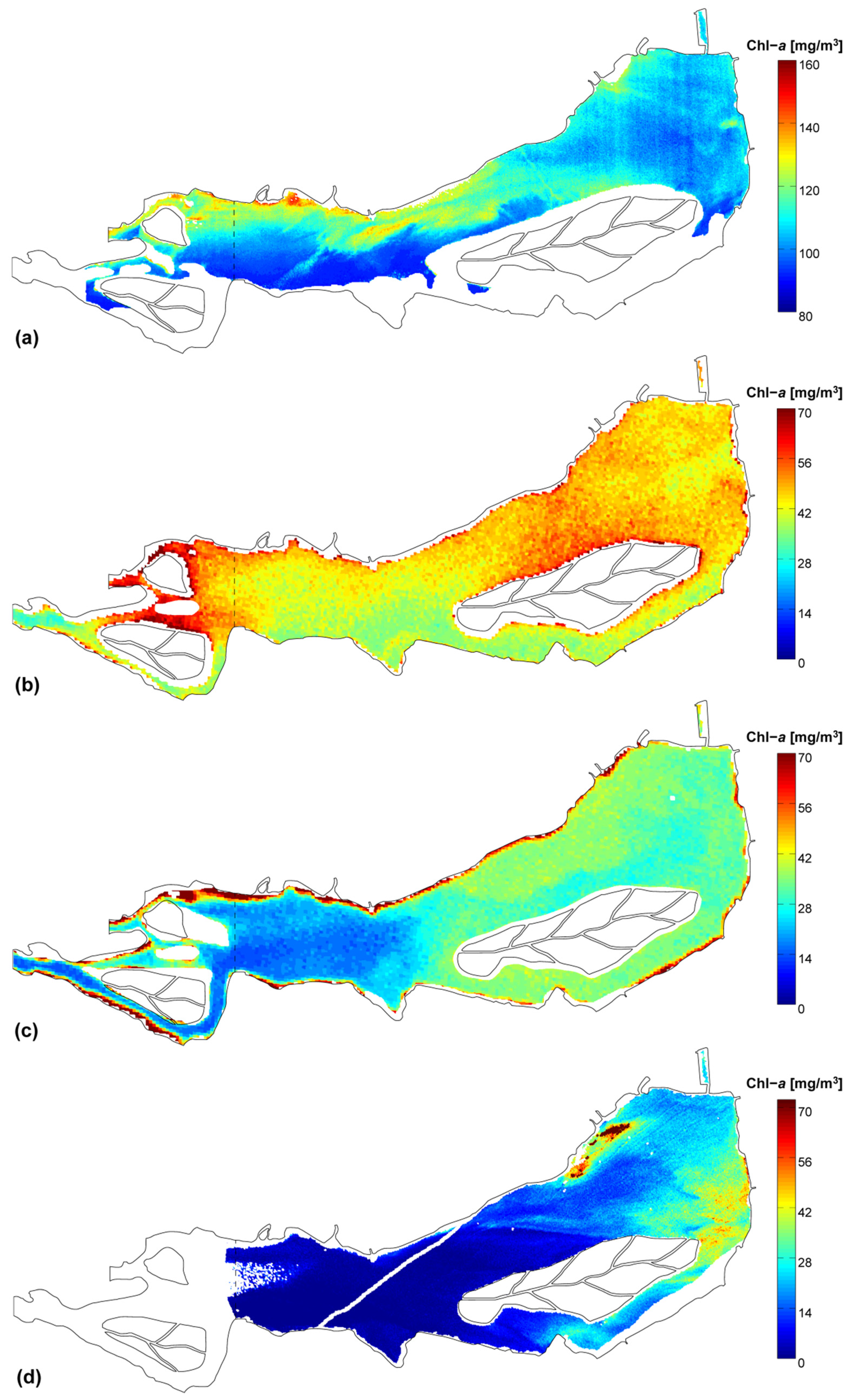
3.2. Chlorophyll-a Distribution Maps

In the MIVIS 26 July 2007 image, Chl-a concentration (Figure 2a) was very high throughout the lake, due to the drought conditions of the Mantua Lakes system during that summer. In particular, the highest Chl-a concentration was registered upstream, in the north-western part of the lake. Unfortunately, remote-sensed chlorophyll-a data for the channel south of the lotus flower island are not available due to a mirror effect.
In the CHRIS-PROBA 29 June 2008 image, Chl-a was also quite evenly distributed throughout the lake, with maximum concentrations observed upstream and in the water canal north of the lotus flower island (Figure 2b). The lowest concentrations were measured instead along the channel south of the macrophyte island. Chlorophyll-a concentration is also quite high in the proximity of the downwind shore.
Both Chl-a distribution maps from 2011 (CHRIS-PROBA 28 August 2011, Figure 2c; APEX 21 September 2011, Figure 2d) showed higher concentrations in the downstream part of the lake, more markedly in the APEX image. In the downstream part of the lake, a corridor with lower Chl-a concentration can be clearly seen along the north side of the lotus flower island, especially in the CHRIS-PROBA image. Chlorophyll-a accumulates nearby the northern shore, in the channel south of the island and downstream of it.
Figure 2. Chlorophyll-a (Chl-a) distribution maps for the MIVIS 26 July 2007 (a); CHRIS-PROBA 29 June 2008 (b); CHRIS-PROBA 28 August 2011 (c) and APEX 21 September 2011 (d) images.
Water 07 01921 g002

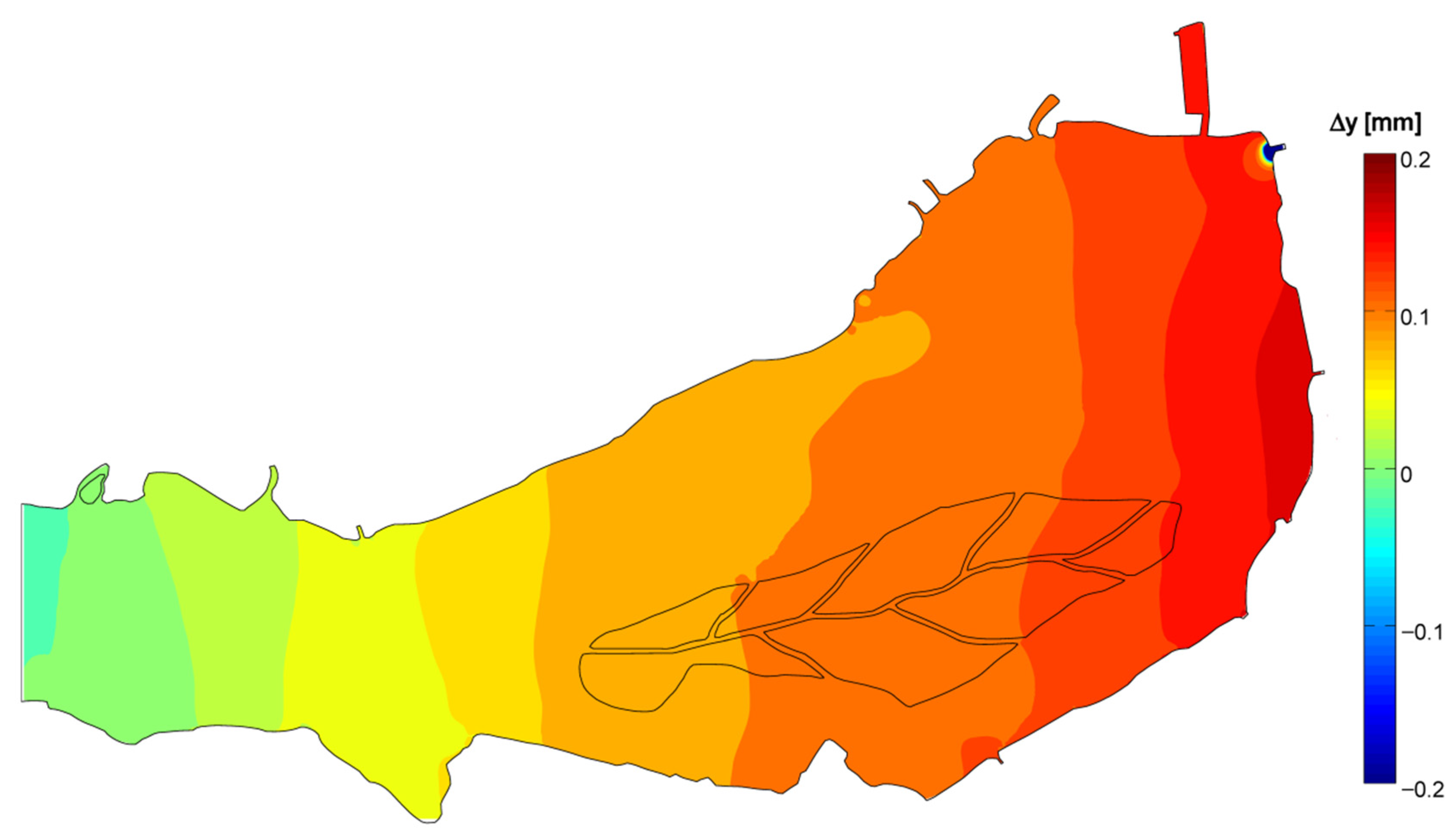
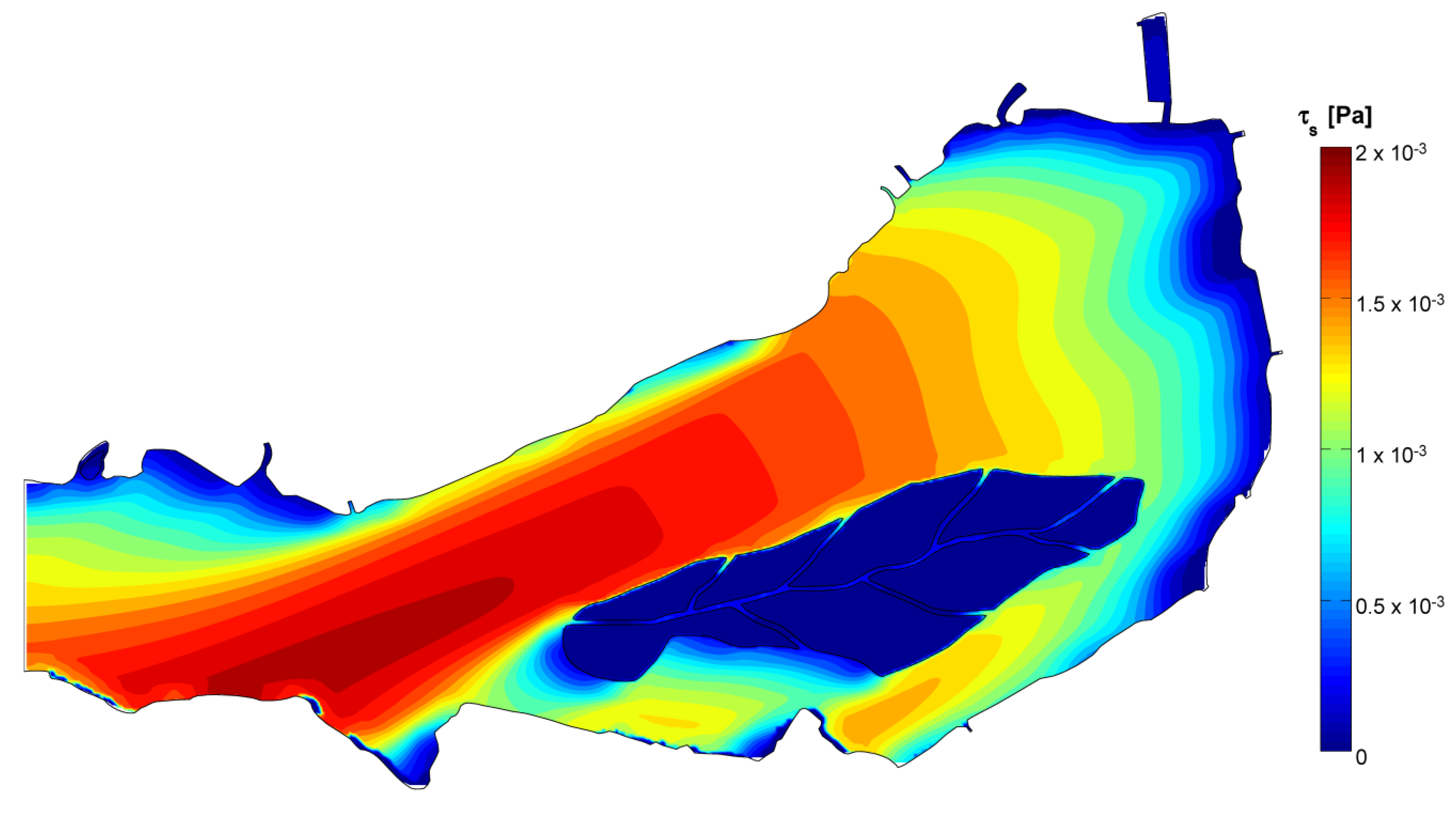
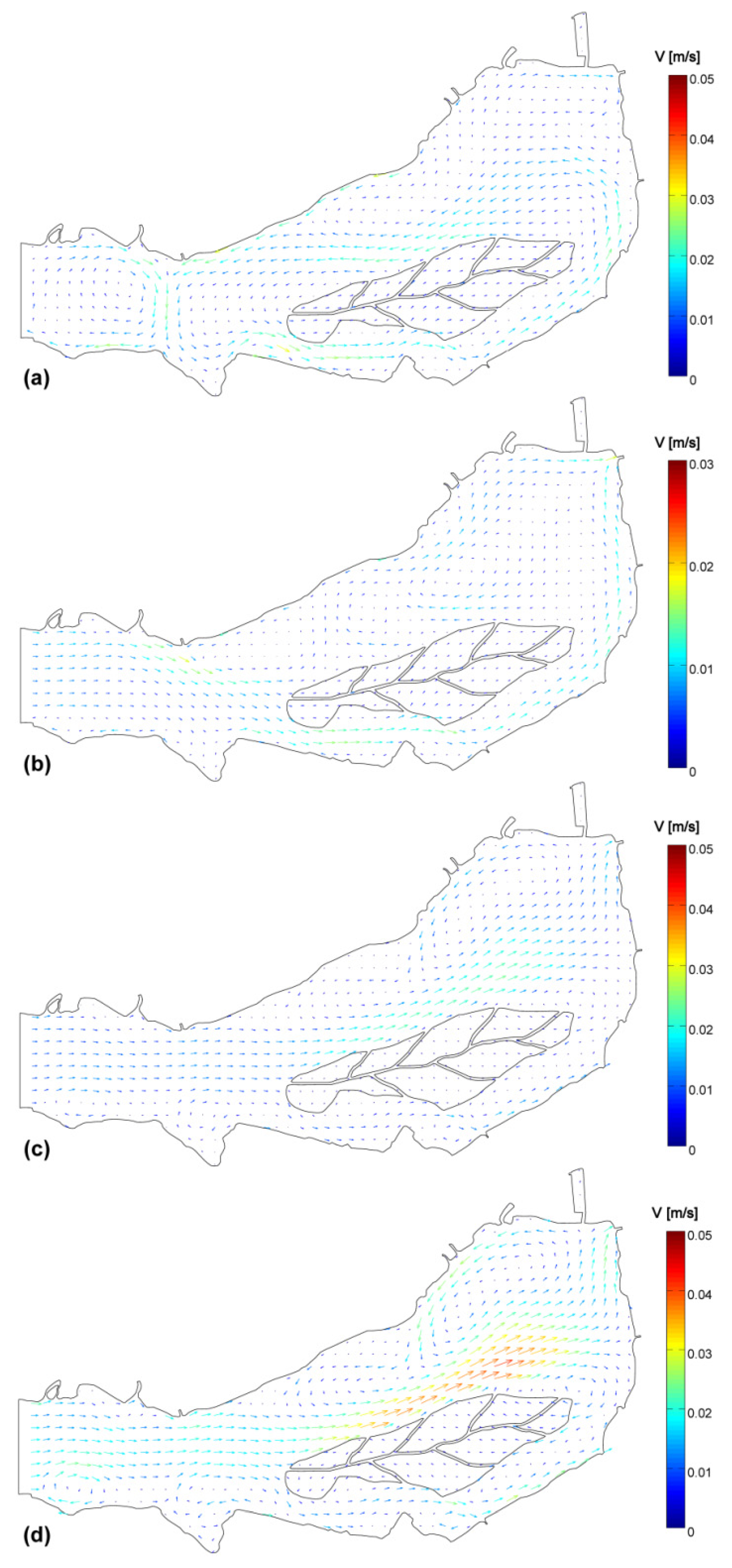
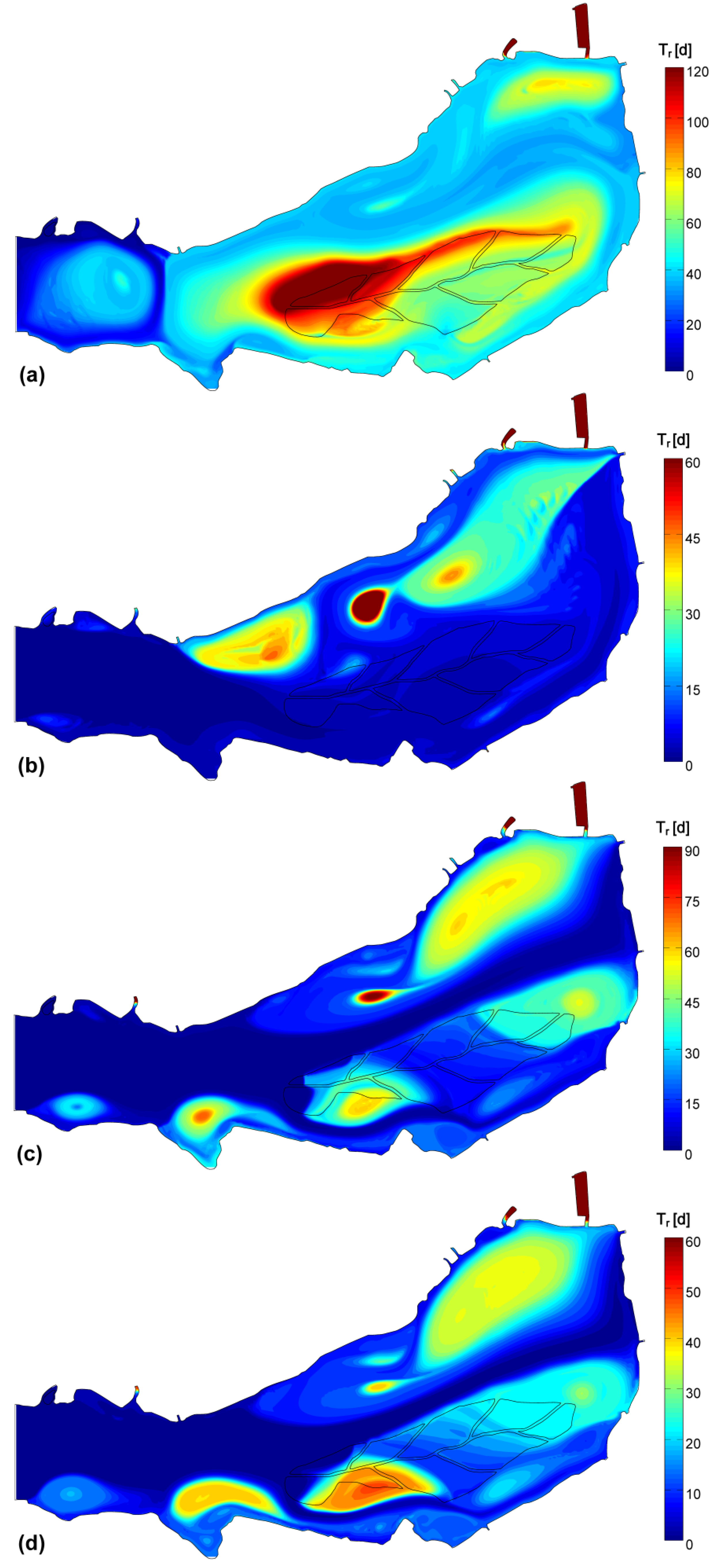
3.3. 3D Hydrodynamic Model

The hydrodynamic variables computed with the 3D model were depth-averaged along the first meter below the free surface only, in order to compare them to the remote-sensed Chl-a data, which are representative of approximately one meter of water depth due to the limited light penetration. The hydrodynamic variables which were found to be related to the chlorophyll-a horizontal patchiness were: water level variations (Δy), wind stress (τs), water velocity direction and its magnitude (V), local water renewal time (Tr).
Water level variations (obtained from pressure deviations) from the control level for the Superior Lake of Mantua of 17.50 m a.s.l., fixed as top elevation for the surface cells, are representative both of wind-induced water displacement, which occurs in the wind direction and is proportional to its intensity, and of flow head losses in the downstream direction, which are proportional to flow discharge: the overlapping of these effects determines the actual surface setup. For the ordinary wind intensities of the analyzed images situations, wind-induced level differences within the model are in the order of 10−4 to 10−3 m, while head losses for the low to average discharge conditions herein examined are in the order of 10−6 to 10−5 m, so that wind action always prevails: the two 2011 simulations with westerly winds show higher water levels downstream (e.g., Figure 3). Surface setup can then be used as a general indicator for the transport direction of the water mass and its associated phytoplankton content.
Figure 3. Water level variations for the CHRIS-PROBA 28 August 2011 simulation.
Water 07 01921 g003
Wind stress according to the adopted IBL model grows in the windward direction, with sheltered areas adjacent to the windward shores, downwind of the lotus flowers island and next to leeward vegetated shores. Simulations of the 2007 and 2008 conditions with easterly winds show higher wind stresses in the upstream part of the lake (e.g., Figure 4), while the opposite occurs in the 2011 cases with westerly winds.
Figure 4. Wind stress field for the CHRIS-PROBA 29 June 2008 simulation.
Water 07 01921 g004
In the MIVIS 2007 conditions with very low discharge, almost non-fluvial lake circulations are obtained (Figure 5a), as a lake-wide counter-clockwise gyre forms around the lotus flower island: an upstream backflow, parallel to the wind direction, is present in the wind-exposed channel north of the island, while a downstream flow forms in the sheltered southern channel. In the upstream part of the lake, a clockwise gyre develops, which limits the development of the main gyre. The exact layout of this upstream gyre may be possibly influenced by the fictitious upstream boundary of the numerical model, but its presence is indeed realistic, because of the differential wind stress between the sheltered northern and the wind-exposed southern shores. Inside the lotus flower island, water flows opposite to the wind, a character common to all simulations because of sheltering. A stagnation area also forms in the downstream part of the lake, north of the large gyre. Local water renewal times are higher inside recirculation areas, especially in the main one, but an almost uniform distribution is attained elsewhere because of low flow and wind-induced circulations (Figure 6a).
In the CHRIS-PROBA 2008 conditions, instead, wind and through-flowing discharge contrast one another in determining the circulations layout (Figure 5b). The riverine current, which is opposite to the wind direction, flows in wind-sheltered areas (Figure 4), first channeling along the northern shore in the upstream part of the lake, then shifting into the channel south of the island and finally flowing towards the Vasarone sluice gate along the downstream shore. Multiple recirculation structures form nearby the northern shore and downstream of the lotus flower island. The local simulated Tr distribution echoes the circulations layout: lower values are attained in the stronger flow areas, higher values in the stagnation regions (Figure 6b).
The 2011 simulations with westerly winds, concordant to the riverine flow direction, give similar results (Figure 5c,d): the flow fields have the same structure, although higher velocity magnitudes are attained in the APEX case because of the higher wind intensity. A river-like behavior is evident in the upstream part of the lake, with a flow parallel to the shores; circulations start to develop where the lake cross section widens. Downstream, the main flow concentrates in the most wind-exposed central region of the lake, north of the lotus flower island. Multiple large recirculation zones develop close to the northern shore, which is sheltered by wind and vegetation. A relevant stagnation area is present about halfway along that shore, caused by a deeper region in the lake bathymetry (Figure 1b). The flow in the channel south of the lotus flower island is much less intense than north of it, especially in its sheltered downstream half. Another stagnation area is present downstream of the island, due to wind sheltering and to wake effect. The local water renewal times are consistent with the described flow field: higher values are obtained inside gyres and in low velocity zones (Figure 6c,d).
Figure 5. Surface 1 m depth-integrated flow fields for the MIVIS 26 July 2007 (a); CHRIS-PROBA 29 June 2008 (b); CHRIS-PROBA 28 August 2011 (c) and APEX 21 September 2011 (d) simulations.
Water 07 01921 g005
Figure 6. Surface 1 m local water renewal times for the MIVIS 26 July 2007 (a); CHRIS-PROBA 29 June 2008 (b); CHRIS-PROBA 28 August 2011 (c) and APEX 21 September 2011 (d) simulations.
Water 07 01921 g006

3.4. Data and Simulation Analyses

Table 4 reports the μ and CV values of the simulated local Tr and of the remote-sensed Chl-a concentrations. The mean values of Tr can be compared to the theoretical water renewal times (also shown in Table 4), obtained as the ratio between the volume of the model (9.68 Mm3) and the discharge. Low values of renewal time CV imply better mixing conditions; the same can be said for the CV of the Chl-a concentration, which also hints at phytoplankton distribution inhomogeneity between the upstream and the downstream part of the lake, owing to advection effects e.g., [10].
Table 4. Theoretical Tr estimates and μ and CV values of simulated Tr and remote-sensed Chl-a concentration for the simulated images conditions.
ParameterMIVIS
26 July 2007
CHRIS-PROBA
29 June 2008
CHRIS-PROBA
28 August 2011
APEX
21 September 2011
Theoretical Tr [d]43.611.211.68.8
Simulated Trμ [d]45.910.020.016.1
CV59%150%129%118%
Remote-sensed Chl-aμ [mg/m3]107.845.932.315.1
CV9%12%30%86%
A qualitative comparison of the simulated hydrodynamic fields to the remote-sensed Chl-a distributions shows that the general characters of the phytoplankton horizontal patchiness can be deduced from the numerical model results.
In the MIVIS 2007 case, the simulated local water renewal time distribution (Figure 6a) is approximately constant, matching with the generally uniform trophic state of the Superior Lake (Figure 2a, see also low CV in Table 4). The higher Chl-a concentration in the upstream part of the lake can be due to wind transport from downstream, in particular along the sheltered northern shore, where currents from upstream and downstream merge (Figure 5a), advecting phytoplankton from both directions. In this area, the small inflow from two drainage channels (not reproduced in the model) can contribute to the formation of local phytoplankton patches due to additional nutrients discharge [9,19]. Phytoplankton accumulation seems to follow the path of the significant backflow induced by the main gyre. The results in the channel south of the lotus flower island are most likely affected by the fact that during summer 2007 the lotus flower island was 35% larger than that reproduced by the model, so that a flow weaker than the simulated one may have occurred in that area (Chl-a data are not available in the image). In fact, a macrophytes control plan was started by local authorities in late 2007, aiming at the reduction of the macrophyte islands extension.
In the CHRIS-PROBA 2008 conditions, the Chl-a concentration field (Figure 2b) results from the contrasting actions of the riverine current, conveying phytoplankton downstream, and of the wind, pushing it upstream. In particular, the mean estimated Tr is even smaller than the theoretical one (Table 4), highlighting how easterly winds produce a better mixing, as opposed to the CHRIS-PROBA 2011 case, which is characterized by similar discharge and wind intensity, but by opposite wind direction (Table 2 and Table 4). Apart from the maximum in the upstream part of the lake, most likely due to wind advection, the highest Chl-a concentrations were observed in correspondence of the deepest part of the lake, where the numerical simulation highlights a central recirculation structure, receiving water from both upstream and downstream (Figure 5b); in the same area, the highest local water renewal times are found (Figure 6b), hence supporting phytoplankton accumulation. The quite high concentration adjacent to the downwind shore may be due to the well-defined flow towards the Vasarone outlet (Figure 5b). The lowest Chl-a concentrations are instead reported, as shown by the simulation, in the sheltered regions where the riverine flow channels.
In the 2011 CHRIS-PROBA and APEX conditions, Chl-a concentrations (Figure 2c,d) were higher in the downstream part of the lake due to the wind action and to the discharge from the Mincio River, with lower values in the upstream riverine part, where the simulations show a channeled flow (Figure 5c,d). Phytoplankton was concentrated further downstream in the APEX image, because of the higher wind intensity (Table 2), resulting in the highest CV value for Chl-a concentration in Table 4. Phytoplankton packed where the strongest backflow develops in the simulation (i.e., nearby the northern shore), as well as in the wind-sheltered downstream half of the channel south of the lotus island and downstream of it, where recirculation structures, weak currents and high local water renewal times (Figure 6c,d) are simulated. Table 4 also shows that the formation of recirculation structures in the downstream part of the lake, where the phytoplankton concentration is the highest, determines the mean simulated local renewal times at almost double the theoretical ones.
The consistency in the identified relations between the hydrodynamic variables and the remote-sensed Chl-a fields suggest that the developed model is indeed robust and validated. However, some limits of the numerical simulations, which are deemed responsible for the deviations between the remote-sensed chlorophyll-a and the hydrodynamic fields, must be acknowledged. First of all, phytoplankton patchiness is the product of transient past processes, of which the steady-state hydrodynamic conditions here assumed are an approximation e.g., [7]. Secondly, a high-resolution bathymetry of the Superior Lake of Mantua, scanned with echosounder techniques, is not available at the present moment, so that the geometry of the numerical model includes some imperfections. The fictitious upstream boundary of the model, which was chosen because of the lack of topographic data for the western part of the lake, also limits the correct development of circulations in the upstream reach of the model. The intrinsic approximations of the schemes used to model the lake physics and the uncertainties in the choice of some of their parameters must be taken into account as well. Moreover, phytoplankton patchiness is remotely conditioned by biochemical factors which, even if acting over long time and very small spatial scales, are not included in the model. Finally, defects in the Chl-a concentration detection algorithms should also be taken into consideration (see Table 1).
The performed analysis suggests that hydrodynamic phenomena determine phytoplankton horizontal patchiness in the Superior Lake of Mantua over three levels:
  • The generalized transport in the wind direction is responsible for major phytoplankton arrangement, as observed, for instance, by George et al. [18]. In the Superior Lake of Mantua, the main wind axis is aligned to the riverine flow, so that, according to the wind direction, the two forces may sum up or oppose one another, resulting either in packing on one of the ends of the lake or in a more uniform distribution.
  • The stagnation in correspondence of gyres traps water and its phytoplankton content, favoring species that prefer motionless waters, such as cyanobacteria [52], to proliferate under stable hydrodynamic conditions. Opposed to this phenomenon are the lower concentrations observed where strong currents develop, because of turbulence disturbance and faster water renewal.
  • The small-scale transport by local currents is responsible for the formation of phytoplankton assemblies on top or outside of the generalized wind advection.
Such hypotheses, deduced from qualitative evaluations, are confirmed by the analysis of the Pearson correlation coefficients between the remote-sensed Chl-a distributions and the simulated hydrodynamic fields, shown in Table 5.
Table 5. Correlation coefficients between the remote sensed Chl-a distributions and the simulated hydrodynamic variables for the simulated images conditions (correlations with p >0.001 are typed in italics).
VariableMIVIS
26 July 2007
CHRIS-PROBA
29 June 2008
CHRIS-PROBA
28 August 2011
APEX
21 September 2011
Δy0.071−0.3680.4550.792
τs−0.055−0.087−0.472−0.193
Tr−0.1750.2760.2150.276
V0.170−0.159−0.1830.008
The calculated values of the correlation coefficients are generally low, due to the aforementioned limits of the numerical model and the non-linearity of the relations between hydrodynamics and phytoplankton patchiness occurring in the real world. However, their sign and the trend of the values over the four cases are meaningful to understand the underlying mechanisms relating the two processes. Elaborate statistical models e.g., [8,15] would better describe the complex, composite and, to a large extent, site-specific relations of the Chl-a concentrations to the hydrodynamic variables. Yet, such an analysis would overcome the purpose of the present research article, which is to demonstrate the feasibility of the use of a hydrodynamic model to forecast the extension and location of the areas of most probable phytoplankton accumulation and the consequent environmental risks in shallow fluvial lakes.
Given the mentioned remarks, quite high positive values are found for the correlation between Chl-a concentration and free surface level variations for the 2011 simulations, in which the downstream water level is higher (e.g., Figure 3) and wind and riverine current advections support one another, proving the major influence of these phenomena. The largest correlation is found for the APEX 2011 case, which is characterized by higher wind and discharge. A weaker positive correlation is obtained for the MIVIS 2007 simulation, as the very low discharge causes more uniform mixing conditions to occur inside the lake because of wind-induced currents (Figure 6a and Table 4). A negative correlation is instead found for the CHRIS-PROBA 2008 simulation: this can be due to the fact that the section in which riverine and wind-related currents clash, advecting phytoplankton from both ends of the lake, is placed in the downstream part of the lake.
Generally weaker negative correlations are found in all cases for the wind stress, showing that wind-sheltered areas (i.e., where wind stress is minimum) are more subject to phytoplankton packing. It must be anyway underlined that in a fluvial lake, such as the one studied here, the riverine through-flowing current tends to channel in wind-sheltered regions, provoking phytoplankton flushing, which may explain the less robust link.
Positive correlations are found in three out of four cases for the simulated local water renewal time, showing the definite effect of water stagnation on phytoplankton packing and proliferation. Small negative correlations are finally found in two cases for velocity magnitude, as phytoplankton tends to accumulate in weak flow areas. In the APEX 2011 simulation, a non-significant correlation is found for this variable. Due to the complexity of the drought condition, it is not immediately evident to explain the opposite correlation of the Chl-a concentration to water velocity and renewal time found for the MIVIS 2007 situation compared to the others. It seems that water stagnation caused phytoplankton decay and that where minimum water flow persisted algae were favored. In this case, the low discharges and higher water renewal times, causing a longer phytoplankton residence inside the lake, may allegedly result in biochemical factors such as photo-inhibition, CO2 or nutrients limitation and prey-predator dynamics to play a relevant role in determining phytoplankton distribution, reducing the physical factors dominance. Under such conditions, therefore, the use of a coupled ecologic-hydrodynamic model may be justifiable.

4. Conclusions

Shallow fluvial lakes are rapidly evolving and menaced ecosystems due to eutrophic conditions coupled to reduced water flows, rapid infilling and occurrence of algal blooms, including potentially harmful cyanobacteria. They are extremely patchy, with a mosaic of very different hydrodynamic, physico-chemical and biological conditions, and for these reasons difficult to analyze comprehensively. This study demonstrates the capabilities of hyperspectral remote-sensing products to validate numerical hydrodynamic lake models, in addition to detect most probable algal blooms location and extension. Remote sensing techniques, despite the still existing spatial resolution limits, may contribute to the monitoring of fluvial lakes, offsetting the limits of occasional, conventional samplings performed on a single location. On the other hand, the costs of airborne campaigns (e.g., MIVIS, APEX) or calibration issues may prevent the mapping of chlorophyll-a in inland waters. Numerical models of lake hydrodynamics, simulating the relevant physical phenomena responsible for the circulations layout, can be used to effectively estimate the environmental risk connected to local stagnation and phytoplankton accumulation (e.g., anoxia events) under given hydrological and meteorological conditions. Relations of the hydrodynamic variables to the Chl-a distribution can be meaningfully assessed by comparing the simulations results to remote-sensed images, providing also an indirect validation of the numerical model, in which the implementation of a variable wind stress model (IBL) has been proved essential to obtain realistic flow fields.
The monitoring and protection of inland water quality may be therefore guaranteed by the integration of ecological, hydraulic, and remote-sensing techniques, with important improvements in management actions by local authorities and policy makers.
The simulation of several flow conditions in the Superior Lake of Mantua, a peculiar fluvial lake case, shows that the main hydrodynamic effects which influence Chl-a distribution are related to the combined effect of advection due to wind force and riverine current, as well as to the presence of large gyres which induce recirculation and stagnation regions, favoring phytoplankton accumulation.

Acknowledgments

The research leading to these results received funding from the European Community’s Seventh Framework Programme [FP7/2007–2013] under grant agreement No. 606865, INFORM project. Thanks to European Facility for Airborne Research (EUFAR) project and VITO for APEX data. MIVIS data were acquired by CGR-CISIG Parma (Italy). CHRIS data were made available through the ESA projects MELINOS (AO-553). We acknowledge ARPA Lombardy and AIPo Mantua office for providing historical wind, biological, physico-chemical data and water discharge data, respectively. We also thank MeteoMincio and the CML for providing the other wind data. The contributions of three anonymous reviewers to the improvement of the original manuscript are likewise acknowledged.

Author Contributions

Monica Pinardi performed the biochemical evaluations, wrote the relative part of the paper and joined the different contributions, writing also the introduction and the conclusions. Andrea Fenocchi developed the hydrodynamic model, conceived the simulations, wrote the connected portion of the manuscript and prepared the figures. Claudia Giardino contributed to the remote-sensing analysis and to the writing of the relative section of the paper. Stefano Sibilla supervised the hydrodynamic modelling as advisor for A. Fenocchi’s Ph.D. and revised the paper. Marco Bartoli participated to the ecological analysis and revised the paper. Mariano Bresciani produced the Chl-a distribution maps and wrote the relative part of the paper.

Conflicts of Interest

The authors declare no conflicts of interest.

References

  1. Teodoru, C.; Wehrli, B. Retention of sediments and nutrients in the Iron Gate I Reservoir on the Danube River. Biogeochemistry 2005, 76, 539–565. [Google Scholar] [CrossRef]
  2. Humborg, C.; Ittekkot, V.; Cociasu, A.; Bodungen, B.V. Effect of Danube River dam on Black Sea biogeochemistry and ecosystem structure. Nature 1997, 386, 385–388. [Google Scholar] [CrossRef]
  3. McCartney, M. Living with dams: Managing the environmental impacts. Water Policy 2009, 11, 121–139. [Google Scholar] [CrossRef]
  4. Bresciani, M.; Rossini, M.; Morabito, G.; Matta, E.; Pinardi, M.; Cogliati, S.; Julitta, T.; Colombo, R.; Braga, F.; Giardino, C. Analysis of within- and between-day chlorophyll-a dynamics in Mantua Superior Lake, with a continuous spectroradiometric measurement. Mar. Freshwater Res. 2013, 64, 303–316. [Google Scholar]
  5. Harris, G.P. Phytoplankton productivity and growth measurements: Past, present and future. J. Plankton Res. 1984, 6, 219–237. [Google Scholar] [CrossRef]
  6. Reynolds, C.S. Scales of disturbance and their role in plankton ecology. Hydrobiologia 1993, 249, 157–171. [Google Scholar] [CrossRef]
  7. Verhagen, J.H.G. Modeling phytoplankton patchiness under the influence of wind-driven currents in lakes. Limnol. Oceanogr. 1994, 39, 1551–1565. [Google Scholar] [CrossRef]
  8. De Souza Cardoso, L.; da Motta Marques, D. Hydrodynamics-driven plankton community in a shallow fluvial lake. Aquat. Ecol. 2009, 43, 73–84. [Google Scholar]
  9. George, D.G.; Heaney, S.I. Factors Influencing the Spatial Distribution of Phytoplankton in a Small Productive Lake. J. Ecol. 1978, 66, 133–155. [Google Scholar] [CrossRef]
  10. Jones, R.I.; Fulcher, A.S.; Jayakody, J.K.U.; Laybourn-Parry, J.; Shine, A.J.; Walton, M.C.; Young, J.M. The horizontal distribution of plankton in a deep, oligotrophic lake—Loch Ness, Scotland. Freshwater Biol. 1995, 33, 161–170. [Google Scholar] [CrossRef]
  11. Ciraolo, G.; Lipari, G.; Napoli, E.; Józsa, J.; Krámer, T. Three-dimensional numerical analysis of turbulent wind-induced flows in the lake Balaton (Hungary). In Shallow Flows—Research Presented at the International Symposium on Shallow Flows, Delft, Netherlands, 16–18 June 2003; Uijttewaal, W.S.J., Jirka, G.H., Eds.; CRC Press/Balkema: Leiden, The Netherlands, 2004. [Google Scholar]
  12. Wiens, J.A. Spatial Scaling in Ecology. Funct. Ecol. 1989, 3, 385–397. [Google Scholar] [CrossRef]
  13. Pinel-Alloul, B. Spatial heterogeneity as a multiscale characteristics of zooplankton community. Hydrobiologia 1995, 104, 17–42. [Google Scholar] [CrossRef]
  14. Legendre, L.; Demers, S. Towards Dynamic Biological Oceanography and Limnology. Can. J. Fish. Aquat. Sci. 1984, 41, 2–19. [Google Scholar] [CrossRef]
  15. Thackeray, S.J.; George, D.G.; Jones, R.I.; Winfield, I.J. Quantitative analysis of the importance of wind-induced circulation for the spatial structuring of planktonic populations. Freshwater Biol. 2004, 49, 1091–1102. [Google Scholar] [CrossRef]
  16. George, D.G. Wind-induced water movements in the South Basin of Windermere. Freshwater Biol. 1981, 11, 37–60. [Google Scholar] [CrossRef]
  17. Livingstone, D.A. On the orientation of lake basins. Am. J. Sci. 1954, 252, 547–554. [Google Scholar] [CrossRef]
  18. George, D.G.; Edwards, R.W. The Effect of Wind on the Distribution of Chlorophyll A and Crustacean Plankton in a Shallow Eutrophic Reservoir. J. Appl. Ecol. 1976, 13, 667–690. [Google Scholar] [CrossRef]
  19. George, D.G.; Winfield, I.J. Factors influencing the spatial distribution of zooplankton and fish in Loch Ness, UK. Freshwater Biol. 2000, 43. [Google Scholar] [CrossRef]
  20. Pinardi, M.; Bartoli, M.; Longhi, D.; Viaroli, P. Net autotrophy in a fluvial lake: the relative role of phytoplankton and floating-leaved macrophytes. Aquat. Sci. 2011, 73, 389–403. [Google Scholar] [CrossRef]
  21. Bolpagni, R.; Bresciani, M.; Laini, A.; Pinardi, M.; Matta, E.; Ampe, E.M.; Giardino, C.; Viaroli, P.; Bartoli, M. Remote sensing of phytoplankton-macrophyte coexistence in shallow hypereutrophic fluvial lakes. Hydrobiologia 2014, 737, 67–76. [Google Scholar] [CrossRef]
  22. Søballe, D.M.; Bachmann, R.W. Influence of reservoir transit on riverine algal transport and abundance. Can. J. Fish. Aquat. Sci. 1984, 41, 1803–1813. [Google Scholar] [CrossRef]
  23. Walz, N.; Welker, M. Plankton development in a rapidly flushed lake in the River Spree system (Neuendorfer See, Northeast Germany). J. Plankton Res. 1998, 20, 2071–2087. [Google Scholar] [CrossRef]
  24. Welker, M.; Walz, N. Plankton dynamics in a river-lake system—On continuity and discontinuity. Hydrobiologia 1999, 408, 233–239. [Google Scholar] [CrossRef]
  25. Rennella, A.M.; Quiros, R. The effects of hydrology on plankton biomass in shallow lakes of the Pampa Plain. Hydrobiologia 2006, 556, 181–191. [Google Scholar] [CrossRef]
  26. Gower, J.F.R.; Denman, K.L.; Holyer, R.J. Phytoplankton patchiness indicates the fluctuation spectrum of mesoscale oceanic structure. Nature 1980, 288, 157–159. [Google Scholar] [CrossRef]
  27. Blauw, A.N.; Los, H.F.J.; Bokhorst, M.; Erftemeijer, P.L.A. GEM: A generic ecological model for estuaries and coastal waters. Hydrobiologia 2009, 618, 175–198. [Google Scholar] [CrossRef]
  28. Salacinska, K.; El Serafy, G.Y.; Los, H.F.J.; Blauw, A. Sensitivity analysis of the two dimensional application of the Generic Ecological Model (GEM) to algal bloom prediction in the North Sea. Ecol. Model. 2010, 221, 178–190. [Google Scholar] [CrossRef]
  29. Mooij, W.M.; Trolle, D.; Jeppesen, E.; Arhonditsis, G.; Belolipetsky, P.V.; Chitamwebwa, D.B.R.; Degermendzhy, A.G.; DeAngelis, D.L.; de Senerpont Domis, L.N.; Downing, A.S.; et al. Challenges and opportunities for integrating lake ecosystem modelling approaches. Aquat. Ecol. 2010, 44, 633–667. [Google Scholar] [CrossRef] [Green Version]
  30. Los, H.F.J.; Villars, M.T.; Van der Tol, M.W.M. A 3-dimensional primary production model (BLOOM/GEM) and its applications to the (southern) North Sea (coupled physical-chemical-ecological model). J. Mar. Syst. 2008, 74, 259–294. [Google Scholar] [CrossRef]
  31. Bresciani, M.; Giardino, C.; Longhi, D.; Pinardi, M.; Bartoli, M.; Vascellari, M. Imaging spectrometry of productive inland waters. Application to the lakes of Mantua. Ital. J. Remote Sens. 2009, 41, 147–156. [Google Scholar] [CrossRef]
  32. Bresciani, M.; Giardino, C.; Bartoli, M.; Longhi, D.; Pinardi, M. Assessment of chlorophyll-a and algal blooms in inland waters from hyperspectral data. In Proceedings of the Hyperspectral 2010 Workshop, ESA SP-683, Frascati, Italy, 17–19 March 2010.
  33. Cutter, M.A. A low cost hyperspectral mission. Acta Astron. 2004, 55, 631–636. [Google Scholar] [CrossRef]
  34. Gitelson, A.A.; Schalles, J.F.; Hladik, C.M. Remote chlorophyll-a retrieval in turbid, productive estuaries: Chesapeake Bay case study. Remote Sens. Environ. 2007, 109, 464–472. [Google Scholar] [CrossRef]
  35. Levasseur, M.; Therriault, J.-C.; Legendre, L. Tidal currents, winds and the morphology of phytoplankton spatial structures. J. Mar. Res. 1983, 41, 655–672. [Google Scholar] [CrossRef]
  36. Józsa, J. On the internal boundary layer related wind stress curl and its role in generating shallow lake circulations. J. Hydrol. Hydromech. 2014, 62, 16–23. [Google Scholar]
  37. Ottesen Hansen, N.-E. Effects of Boundary layers on mixing in small Lakes. Dev. Water Sci. 1979, 11, 341–356. [Google Scholar]
  38. Krámer, T. Solution-Adaptive 2D Modelling of Wind-Induced Lake Circulation. Ph.D. Thesis, Budapest University of Technology and Economics, Budapest, Hungary, 2006. [Google Scholar]
  39. Coastal Engineering Research Center (CERC). Shore Protection Manual, 4th ed.; Waterways Experiment Station: Vicksburg, MS, USA, 1984. [Google Scholar]
  40. Józsa, J. Shallow Lake Hydrodynamics—Theory, Measurement and Numerical Model Applications; Mundus-Euroaquae lecture notes; Budapest University of Technology and Economics: Budapest, Hungary, 2006. [Google Scholar]
  41. CD-adapco. STAR-CCM+ 9.02 User Guide; online manual; CD-adapco: Melville, NY, USA, 2014. [Google Scholar]
  42. Shih, T.H.; Liou, W.W.; Shabbir, A.; Yang, Z.; Zhu, J. A New k-ε Eddy Viscosity Model for High Reynolds Number: Model Development and Validation; NASA Technical Memorandum 106721; NASA Lewis Research Center: Cleveland, OH, USA, 1994.
  43. Teeter, A.M.; Johnson, B.H.; Berger, C.; Stelling, G.; Scheffner, N.W.; Garcia, M.H.; Parchure, T.M. Hydrodynamic and sediment transport modeling with emphasis on shallow-water, vegetated areas (lakes, reservoirs, estuaries and lagoons). Hydrobiologia 2001, 444, 1–23. [Google Scholar] [CrossRef]
  44. Zinke, P. Application of a porous media approach for vegetation flow resistance. In River Flow 2012, San José, Costa Rica, 5–7 September 2012; Murillo Muñoz, R., Ed.; CRC Press/Balkema: Leiden, The Netherlands, 2012. [Google Scholar]
  45. Grant, W.D.; Madsen, O.S. Combined wave and current interaction with a rough bottom. J. Geophys. Res. 1979, 84, 1797–1808. [Google Scholar] [CrossRef]
  46. Dickman, M. Some effects of lake renewal on phytoplankton productivity and species composition. Limnol. Oceanogr 1969, 14, 660–666. [Google Scholar] [CrossRef]
  47. Krivtsov, V.; Sigee, C. Importance of biological and abiotic factors for geochemical cycling in a freshwater eutrophic lake. Biogeochemistry 2005, 74, 205–230. [Google Scholar] [CrossRef]
  48. Yamamuro, M.; Hiratsuka, J.; Ishitobi, Y.; Hosokawa, S.; Nakamura, Y. Ecosystem shift resulting from loss of eelgrass and other submerged aquatic vegetation in two estuarine lagoons, Lake Nakaumi and Lake Shinji, Japan. J. Oceanogr. 2006, 62, 551–558. [Google Scholar] [CrossRef]
  49. Ekholm, P.; Malve, O.; Kirkkala, T. Internal and external loading as regulators of nutrient concentrations in the agriculturally loaded Lake Pyhajarvi (southwest Finland). Hydrobiologia 1997, 345, 3–14. [Google Scholar] [CrossRef]
  50. Burger, D.F.; Hamilton, D.P.; Pilditch, C.A.; Gibbs, M.M. Benthic nutrient fluxes in a eutrophic, polymictic lake. Hydrobiologia 2007, 584, 13–25. [Google Scholar] [CrossRef]
  51. Luettich, R.A.; Harleman, D.R.F.; Somlyody, L. Dynamic Behavior of Suspended Sediment Concentrations in a Shallow Lake Perturbed by Episodic Wind Events. Limnol. Oceanogr. 1990, 35, 1050–1067. [Google Scholar] [CrossRef]
  52. Becker, V.; de Souza Cardoso, L.; da Motta Marques, D. Development of Anabaena Bory ex Bornet & Flahault (Cyanobacteria) blooms in a shallow, subtropical lake in southern Brazil. Acta Limnol. Bras. 2004, 16, 306–317. [Google Scholar]

