Comparative Analysis of Spatial Interpolation Methods in the Mediterranean Area: Application to Temperature in Sicily

Abstract

An exhaustive comparison among different spatial interpolation algorithms was carried out in order to derive annual and monthly air temperature maps for Sicily (Italy). Deterministic, data-driven and geostatistics algorithms were used, in some cases adding the elevation information and other physiographic variables to improve the performance of interpolation techniques and the reconstruction of the air temperature field. The dataset is given by air temperature data coming from 84 stations spread around the island of Sicily. The interpolation algorithms were optimized by using a subset of the available dataset, while the remaining subset was used to validate the results in terms of the accuracy and bias of the estimates. Validation results indicate that univariate methods, which neglect the information from physiographic variables, significantly entail the largest errors, while performances improve when such parameters are taken into account. The best results at the annual scale have been obtained using the the ordinary kriging of residuals from linear regression and from the artificial neural network algorithm, while, at the monthly scale, a Fourier-series algorithm has been used to downscale mean annual temperature to reproduce monthly values in the annual cycle.

1. Introduction

Climatic data are used for scientific and technical purposes in many different areas of environmental research and resource management [1], hydrology and agriculture [2].

Climate series are often limited in spatial and temporal coverage. The management and maintenance of gauge stations to obtain reliable data can be very expensive and problematic. In order to tackle this problems, it is useful to develop spatial interpolation techniques to assess climatic variables at ungauged sites. In general, spatial interpolation techniques use observations of the same variable made at other sites. The methods used to estimate precipitation and temperature at ungauged sites can be grouped into: (I) weighting methods which, in turn, can be classified into deterministic interpolation methods (inverse distance weighting, non-linear interpolation as spline techniques, etc.) and statistic interpolation methods (different varieties of kriging); and (II) data-driven methods (regression, artificial neural networks, etc.) [3].

Even though spatial interpolation techniques have been largely analyzed and compared, an optimum spatial interpolation algorithm is difficult to identify. Indeed, the suitability of a spatial interpolator is strongly related to the specific variable considered, the specific context and the spatial scale desired for mapping [4–7]. Moreover, other factors may also influence the choice of the interpolation method and the accuracy of the results. Among these, station density [8], the duration and the nature of the climate variable [9] (e.g., temperature and sea level pressure are continuous in both time and space, whereas precipitation fields are spatially discontinuous on shorter timescales and more continuous on longer timescales), and geographical factors, such as elevation [10], aspect and distance to the coast [11], are probably the most important. The comparison among algorithms based on deterministic and data-driven methods or methods that integrate stochastic and regressive approaches has usually demonstrated the superiority of the latter two approaches, making them a good solution to the spatial interpolation of climatological variables [12–14].

Among data-driven algorithms, the regression methods can be considered as direct and explicit procedures. These methods use ancillary geographical information as independent variables to improve the estimation of the spatial distribution of the considered climate variables. Several studies present GIS-based spatial interpolation algorithms in order to derive tools for the analysis and the characterization of the spatial structure of precipitation for different applications [15]. Claps et al. [16] applied regression analysis to annual and monthly average temperatures to characterize the temperature regime in Italy. Data from 738 weather stations were used to estimate the temperature normals. In particular geo-regressive methods were used, taking into account geographic and morphological parameters, and through a stepwise regression analysis, the significant variables were detected. The temperature regime was reproduced with a two-harmonic Fourier series, leading to satisfactory results for large-scale climatic characterization.

Another data-driven algorithm widely used to derive the spatial distribution of climatic data is the artificial neural network (ANN) [17,18]. Among the applications of this approach, Rigol et al. [19] used a feed-forward back-propagation network method for the interpolation of geographical data that incorporated both trend and spatial association and applied the method to the daily minimum temperatures in England and Wales. Coulibaly and Evora [20] performed a comparison of six different types of ANN techniques for assessing precipitation and temperature at ungauged sites. The evaluation of the accuracy of the different models, carried out using daily series from 15 validation weather stations, highlighted that multi-layer perceptron (MLP) was the most effective method.

Several geostatistical methods have been used for assessing the performances of the spatial processing of precipitation fields in several works focused on this issue, e.g., [21–23]. As highlighted by Haining et al. [24], geostatistical methods can be used to perform the characterization of the spatial structure of the process considered and provide useful insights into the uncertainty associated with the interpolation analysis. Hudson and Wackernagel [25] analyzed the spatial structure of mean temperature using variograms computed for different directions. Since this anisotropic variogram for universal kriging does not fully explain the spatial variation in temperature, the authors exploited the correlation with elevation, adopting the kriging with elevation as external drift, obtaining better results.

Geostatistics were also used together with ANNs. In particular, Demyanov et al. [26] proposed a two-step spatial interpolation method named direct neural network residual kriging: the first step is a data-driven approach, which includes estimating the large-scale spatial structure by an ANN, while the second step is the analysis of residuals carried out by using a geostatistical method; final estimates are produced as a sum of ANN estimates and ordinary kriging estimates of residuals. A similar approach was followed by Antonic and Krizan [27], who built empirical models based on neural networks for seven climatic variables using 127 weather stations; the residuals coming from the ANN were spatially interpolated by kriging and used as a model correction.

In order to obtain yearly averaged temperature maps providing complete and continuous information in the territory, several algorithms of spatial interpolation are presented and applied in this study to annual and monthly average temperature data of Sicily (Italy) measured at 84 sites. Considering the relevant role of elevation in estimating temperature, e.g., [28,29], a set of specific data-driven and regressive approaches have been chosen. In these methods, the elevation information, as well as other physiographic information, provided by a digital elevation model (DEM), were added to improve the estimation of missing data. Moreover, simple univariate methods have been considered in order to compare their performances with those of more complex methodologies, evaluating the improvements. These different models were first calibrated using a modeling subset and then compared through a validation procedure. Finally, the best method was used to derive maps of annual and monthly average temperature, aiming at the preparation of a climate atlas for Sicily.

2. Methods and Study Area

The selection of methods has been performed in order to exploit the range of interpolators features and potentialities. Following the considerations reported above, methods have been classified among univariate methods and variable aided methods. Among univariate methods, the inverse distance weighting (IDW) has been selected as the most simple spatial interpolation procedure. The radial basis functions (RBF) provide a general mathematical tool that is able to identify a continuous surface representing the variable behavior. Ordinary kriging (OK) has been selected as the method for the exploitation of the spatial variability, as can be observed by means of specific tools, such as the semivariogram. The evaluation of variable-aided interpolators has been first explored with simple linear regression models. Later, more complex methods have been tested. In particular, the geographically-weighted regression has been applied in order to consider the spatial variability of the regressive relationship, and the ANN has been chosen because it is able to model the non-linear relationship between variables. Finally, residual kriging has been explored across different base variable-aided methods in order to evaluate the effects of further modeling the residual variability by means of other methods. Analyses have been performed using ESRI ArcGIS and MATLAB software.

2.1. Climatic and Geographic Features of the Area

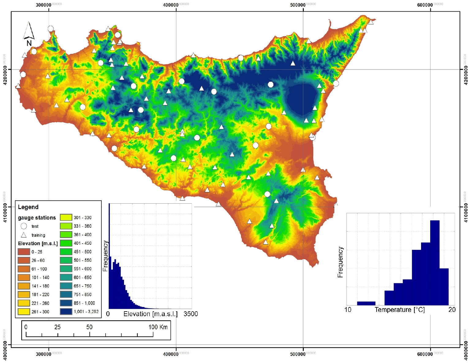
This study concerned the largest island in the Mediterranean Sea, Sicily (Italy), extending over an area of 25,700 km². The ancillary information regarding elevation was embedded through the use of a DEM of the region having a resolution of 100 m (Figure 1). The surface of the island is mainly characterized by a hilly morphology (62%) and, for the rest, by a mountainous and flat morphology among which the widest is around Catania, in the eastern part of the island. The overall island average elevation is around 400 m, but the range of variation of elevation is between 0 and 3263 m (the Etna volcano, the highest peak of Sicily).

Sicily is a region with a temperate-mesothermal (Mediterranean) climate, with a dry summer, having an average temperature in the hottest month greater than 22 °C, with a precipitation regime more intense in the coldest season.

Some physiographic parameters were also considered in this study in order to evaluate their relationship with temperature measurements. Following the criteria of Prudhomme and Reed [30], such physiographic and geographic factors, chosen taking into account the temperature pattern over the area, are the minimum absolute distance from the sea, d_min, the angle α formed by the minimum distance vector and the south, the distance d_i from the sea in the eight cardinal directions i and the azimuthal angle β_i of the horizon in the eight cardinal directions.

The latter variable is the obstruction factor [31], defined as the angle subtended by the highest topographical barrier in the i-th direction, such that tan(β_i) = ΔH/ΔX, with ΔH as the difference of elevation between the barrier and the station, and ΔX as the distance between the two points. These variables have been derived using spatial analysis techniques in a GIS environment, using a vector representation of the Sicilian coastal line and the DEM. These variables were used to produce the three following parameters:

• - the distance measure, D_s, that is the geometric mean of the distance from the sea in the eight cardinal directions:

  $$D_s=\sqrt[8]{d_1\ast d_2\ast \dots \ast d_8}$$

  (1)

• - the aspect variable, A_s, a combined measure of aspect orientation and sea proximity:

  $$A_s=\frac{10\mathit{cos}\mathrm{\alpha }}{1+d_{\mathit{min}}}$$

  (2)

• - the concavity index, C, obtained by weighting the azimuthal angle iin the eight directions:

  $$C=\sqrt[8]{{\displaystyle \prod _{i=1}^8{10}^{2\mathit{tan}{\mathrm{\beta }}_i}}}$$

  (3)

2.2. Climatic Dataset

The temperature dataset used in this study was provided by OA-ARRA (Osservatorio delle Acque-Agenzia Regionale dei Rifiuti e delle Acque) and comes from 84 weather stations with observations recorded from 1924 to 2006. The entire station dataset was divided into two subsets: (I) the modeling subset, used to calibrate the different interpolation methods, containing about 70% of the stations (N_t = 59); and (II) the validation subset, used to validate the calibration results, containing the remaining 30% of the stations (N_v = 25). The partition of the dataset into two subsets was done by trying to maintain the distribution of sites, both in the horizontal domain and in the altitudinal distribution.

In order to provide the estimate $\widehat{z}$ of the temperature variable z, both annual or monthly, at an ungauged location x₀ using temperature data at instrumented sites, denoted with {z (x_i), i = 1, 2, ….N}, the temperature vector measured at the N sites x_i, two different classes of interpolators were used: univariate methods and variable-aided interpolation (VAI) methods. While the former class takes into account only the data and the spatial coordinates x_i, the latter also uses supplementary data, such as elevation q (x_i), and other physiographic variables. These methods will be shortly described in the following subsections.

2.3. Univariate Interpolators

The radial basis function [32] represents a large family of exact interpolators similar to those used in geostatistical interpolation (see further), but without the benefit of a prior analysis of spatial correlation. These interpolators, which do not make any assumption on the input data and provide excellent interpolators for a wide range of data, have been used in many disciplines. The simplest variant of this method can be viewed as a weighted linear function of (inverse) distance from grid point to data point, plus a “bias” factor. The temperature at an ungauged site x₀ can be estimated by:

$$\widehat{z}({\mathit{x}}_0)={\displaystyle \sum _{i=1}^N{\mathrm{\lambda }}_i\mathrm{\varphi }(\Vert {\mathit{x}}_i-{\mathit{x}}_0\Vert )+\mathrm{\mu }}$$

(4)

where ϕ (ρ) is the selected radial basis function, ρ is the radial distance from point x₀ to the i-th data point x_i (ρ = ║x_i − x₀║) and λ_i are the weights to be estimated together with the bias value μ (or Lagrangian multiplier). These weights are given by the solution of a system of (n + 1) linear equations. The radial basis function used in this work is the thin plate spline, which has the following expression:

$$\mathrm{\varphi }(\mathrm{\rho })=c^2{\mathrm{\rho }}^{2}ln(c\mathrm{\rho })$$

(5)

This interpolation method requires the choice of a minimum number of neighbor points.

The second univariate method taken into account here was the inverse distance weighting (IDW). The temperature is a linear combination of several surrounding observations, while the weights are proportional to the distance between observations and x₀:

$$\widehat{z}({\mathit{x}}_0)={\displaystyle \sum _{i=1}^N{\mathrm{\lambda }}_{i}z({\mathit{x}}_i)}$$

(6)

where the weights λ_i are expressed as a function of distance as follows:

$${\mathrm{\lambda }}_i=\frac{d_{i^0}^{-r}}{{\displaystyle \sum _{i=1}^N{d}_{i^0}^{-r}}}$$

(7)

This exact interpolation method requires the choice of the exponent r and of a search radius R or the minimum number of points N.

The third univariate method taken into account, is OK, which belongs to geostatistical interpolators [33,34]. This method uses a particular function, called the semivariogram, instead of simple Euclidean distance functions in order to measure the dissimilarity between observations. The experimental semivariogram is a function of both distance and direction. If anisotropic spatial patterns exist, different semivariograms should be computed along different directions. The semivariogram is used to derive the weights of an unbiased linear interpolator by means of the minimization of the error estimate variance. Thus, the OK can be labeled as a BLUE method (best linear unbiased estimator). The relationship between such weights and the semivariogram results:

$$\overline{\overline{\mathrm{\gamma }}}=\overline{\mathrm{\Gamma }}\cdot \overline{\mathrm{\lambda }}$$

(8)

where $\overline{\mathrm{\gamma }}$ is the semivariogram vector relative to each sample point and that to which the estimation is referred, $\overline{\overline{\mathrm{\Gamma }}}$ is the semivariogram matrix relative to sample points and $\overline{\mathrm{\lambda }}$ is the weight vector relative to the point to be estimated. A detailed characterization of this topic can be found, for instance, in Kitanidis [34], Goovaerts [35].

2.4. Variable-Aided Interpolators

2.4.1. Linear Models

The most simple method belonging to VAI methods is linear regression (LR). It consists of temperature estimation as a function of the elevation of the instrumented sites q (x₀), in the case of simple linear regression, or as a function of more than one physiographic variable, in the case of multiple linear regression (MLR). The equation used for simple and multiple linear regressions is:

$$\widehat{z}({\mathit{x}}_0)=f[v_j({\mathit{x}}_0)]=\mathrm{\alpha }+{\displaystyle \sum _{j=1}^{n_v}{\mathrm{\beta }}_j{v}_j({\mathit{x}}_0)}$$

(9)

where v_j (x₀) are the n_v independent variables for the MLR (n_v = 1 simple regression), while the regression coefficients α, β (or β_j), constant over the whole study area, can be estimated, using the least squares method, from the set of temperature and the independent variables data at N ungauged sites {z (x_i), v (x_i), i = 1, 2, …, N}.

In order to assess regression coefficients, the standard OLS (ordinary least squares) methodology has been compared with the results provided by the robust regression method (ROB) [36]. Physiographic and geographic parameters used in MLR were the elevation q, the latitude L, the minimum absolute distance from the sea, d_min, the angle α formed by the minimum distance vector and the south, the distance d_i from the sea in the eight cardinal directions i, the azimuthal angle β_i of the horizon in the eight cardinal directions and three indices D_s, A_s, C, as previously defined in Equations (1)–(3), respectively.

2.4.2. Geographically Weighted Regression

Geographically Weighted Regression (GWR) [37] considers the variability of coefficients α and β of a regression expression linking temperature to the topographic features allowing these two parameters to change over space using the following relationship:

$$\widehat{z}({\mathit{x}}_0)=f[q({\mathit{x}}_0)]=\mathrm{\alpha }({\mathit{x}}_0)+\mathrm{\beta }({\mathit{x}}_0)q({\mathit{x}}_0)$$

(10)

Each coefficient may be thought of as a 3D surface over the geographical study area rather than a single constant value. The estimation of the two coefficients α (x₀) and β (x₀) can be carried out by one of the two following approaches: GWR with fixed spatial kernels and GWR with adaptive spatial kernels. The latter approach, used in this study, is based on a circle of radius R drawn around a point to calibrate an ordinary least squares regression model on the basis of the observations that fall within this circle; the coefficients α and β are an estimation of the local coefficients at the point x₀. The spatial kernel can be adapted depending on the density of the data [38].

2.4.3. Artificial Neural Networks

ANNs have been extensively applied in the past decade for estimating and forecasting hydrological variables [39,40]. In this work, the MLP method has been applied. An MLP is a feedforward neural network consisting of a number of units (perceptrons or neurons), which are connected by weighted links. The units are organized in layers: an input layer, with a number of neurons defined by the input independent variables, an output layer, with a number of neurons defined by the dependent variable, and, finally, one or more hidden layers. In an MLP, an arbitrary input vector is propagated forward through the network, where the hidden layers of neurons make a linear combination of input signals and convert it through a generally nonlinear function (activation function). Each layer output forms the input to the following layers.

MLP was used like a VAI technique to estimate temperature values at ungauged sites using the elevation information, as well. The implemented MPL consists of three layers: the input layer with three neurons, the output layer with one neuron and one hidden layer.

ANN techniques require a training stage, to learn the dynamics of the causal relationship. In the training phase of an MLP, known input-output pairs are presented to the network, and the weights are updated by following pre-determined learning rules. In our work, the “error backpropagation rule” (EBP) was used.

2.4.4. Use of Residual Spatial Interpolation (Residual Kriging)

The above-mentioned VAI methods (LR, MLR, GWR and ANN) can provide, for each one of the N gauged sites, a residual error defined as the difference between the estimated value ${\widehat{z}}_A({\mathit{x}}_i)$ and the observed value z(x_i):

$$r_A({\mathit{x}}_i)={\widehat{z}}_A({\mathit{x}}_i)-z({\mathit{x}}_i)withA=LR,MLR,GWR,ANNandi=1,2,\dots ,N$$

(11)

The spatial correlation of residuals r_A (x_i) can be taken into account using a geostatistical algorithm denoted as residual kriging (RK). In this case, the four methods estimate large-scale structures of temperature data, valid for the whole domain, and then, the interpolation of residuals r_A(x_i), carried out with the OK method, produces a map of r_A(x_i) representing the corrections to apply to each one of the three models. Final estimates at an ungauged site x₀ are produced as a sum of the VAI method estimates and ordinary kriging estimates of residuals:

$${\widehat{z}}_{RK-A}({\mathit{x}}_0)={\widehat{z}}_A({\mathit{x}}_0)+{\widehat{r}}_A({\mathit{x}}_0)withA=LR,MLR,GWR,ANN$$

(12)

This approach has been extensively used for mapping climatic variables [21,30,41].

2.5. Fitting Monthly Temperature by Fourier Series

Another method, based on the seasonal scaling of annual temperature, was implemented in the case of monthly analysis. This method, described in Claps et al. [16], allows one to derive the monthly temperature by means of the estimation of the whole parameterized curve of the temperature regime at each point over the domain. With such an approach, it is possible to describe with a single model the causal relationship between physiographic and geographic predictors and the seasonality of temperature in Mediterranean climates. Starting from estimates of the spatial variability of the mean annual temperatures, the monthly deviations from the annual mean can be analyzed, considering the zero-mean temperature regime t (j) given by this expression:

$$t(j)=T(j)-T_a$$

(13)

where j denotes the month of the year, T(j) is the average temperature at month j and T_a is the mean annual temperature. The sequence of 12 monthly temperature deviations t (j) can be well approximated by means of sinusoidal curves obtained by Fourier series using the following expression:

$$t(j)=A_0+{\displaystyle \sum _{i=1}^N{A}_i\mathit{cos}\left(\frac{2\mathrm{\pi }}{\mathrm{\tau }}j+\frac{\mathrm{\tau }}{{\mathrm{\tau }}_i}{\mathrm{\varphi }}_i\right)}$$

(14)

where A₀ is the mean of t (j) (here, equal to zero), τ, here equal to 12, is the fundamental period of the cycle, N is the number of the harmonics, A_i is the amplitude, ϕ_i is the phase and τ_i is the period of the i-th harmonic. For the estimation of the Fourier series parameters, the cosine argument in Equation (14) can be decomposed to a polynomial form:

$$t(j)=A_0+{\displaystyle \sum _{i=1}^N\left[b_i\ast \mathit{cos}\left(\frac{2\mathrm{\pi }}{12}j\right)+c_i\ast sin\left(\frac{2\mathrm{\pi }{n}_i}{12}j\right)\right]}$$

(15)

where b_i = A_icos (n_iϕ_i); c_i = −A_icos (n_iϕ_i), and $\frac{\mathrm{\tau }}{{\mathrm{\tau }}_i}$. The amplitude and phase of the i-th harmonic can then be obtained as:

$$A_i=\frac{b_i}{\mathit{cos}(n_i{\mathrm{\varphi }}_i)}$$

(16)

$${\mathrm{\varphi }}_i=arc\mathit{tan}\left(-\frac{c_i}{b_i}\right)$$

(17)

2.6. Evaluation of Different Algorithms

For a general comparison among methods, it was not possible to use the geostatistical cross-validation [33] because of the presence of global interpolation methods, such as LR and GWR. Therefore, the comparison criteria were based on the following different indices used to measure the strength of the statistical relationship between estimated $\widehat{z}({\mathit{x}}_i)$ and measured z (x_i) temperatures in the N_v points of the validation subset.

• The RMSE (root mean square error of the prediction), which measures the average square difference between the true temperature and its estimate at the validation points:

  $$RMSE=\sqrt{\frac{1}{N_v}{\displaystyle \sum _{i=1}^{N_v}{[\widehat{z}({\mathit{x}}_i)-z({\mathit{x}}_i)]}^2}}$$

  (18)

• The MBE (mean bias error) or simply bias:

  $$MBE=\frac{1}{N_v}{\displaystyle \sum _{i=1}^{N_v}[\widehat{z}({\mathit{x}}_i)-z({\mathit{x}}_i)]}$$

  (19)

• The MAE (mean absolute error):

  $$MAE=\frac{1}{N_v}{\displaystyle \sum _{i=1}^{N_v}[\left|\widehat{z}({\mathit{x}}_i)-z({\mathit{x}}_i)\right|]}$$

  (20)

• The CC (linear correlation coefficient):

  $$CC=\frac{{\displaystyle {\sum }_{i=1}^{N_v}[z({\mathit{x}}_i)-z_m][\widehat{z}({\mathit{x}}_i)-{\widehat{z}}_m]}}{{\mathrm{\sigma }}_e{\mathrm{\sigma }}_o{N}_v}$$

  (21)
  where z_m and ${\widehat{z}}_m$ are the mean of measured and estimated temperature values, respectively, and σ_e and σ_o are the standard deviation of measured and estimated temperature values, respectively.

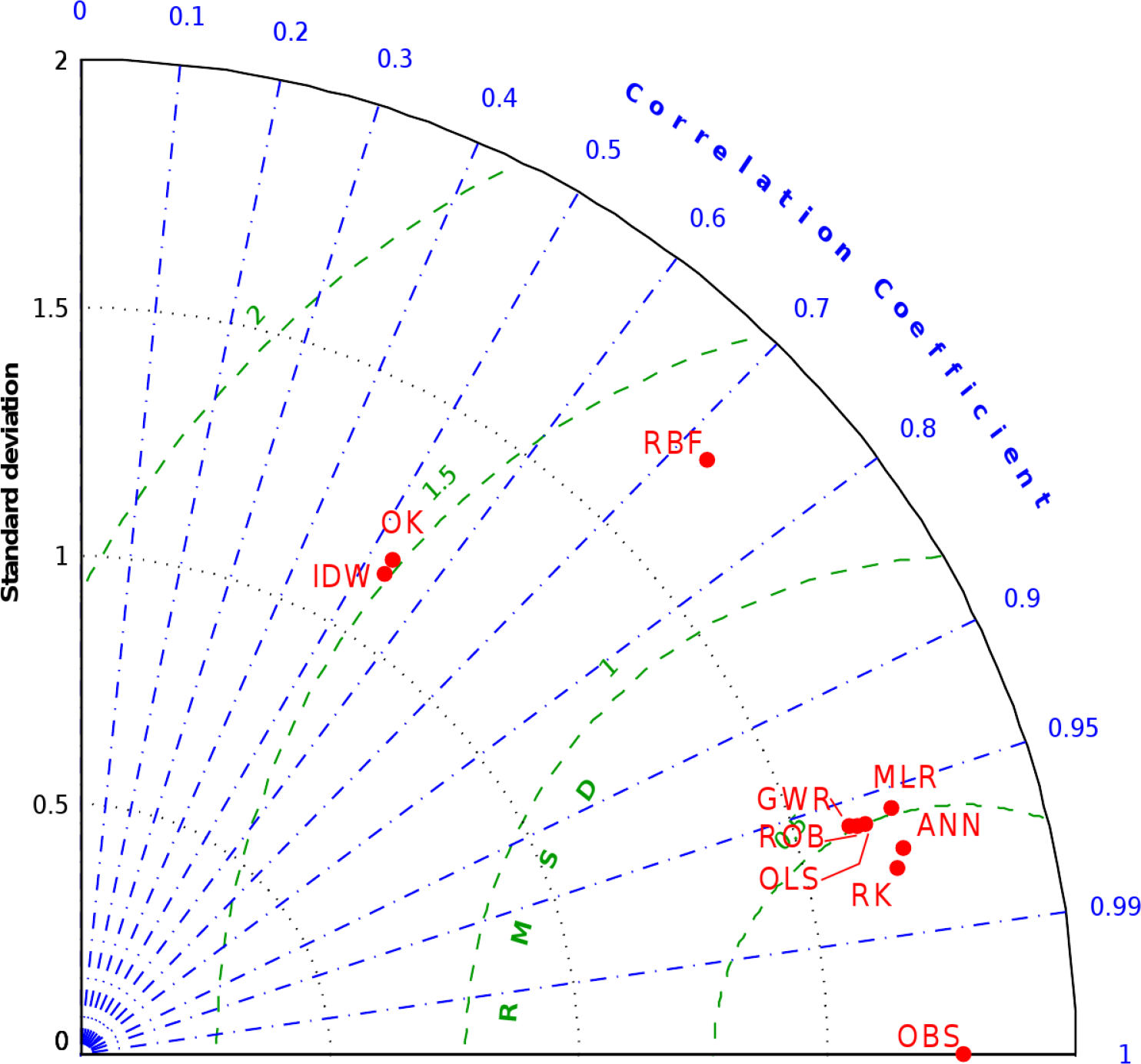
Another tool used to compare the different methods is the Taylor diagram [42]. This tool is based on a trigonometric similitude between the standard deviation of series (SD), CC and centered pattern root mean square difference (RMSD), and it allows the measuring of estimate performances, in terms of RMSD, given SD and CC values calculated between estimates and measurements for the validation subset.

3. Results

3.1. Univariate Methods

The application of the first univariate method, RBF with a thin plate spline, has been performed by varying the minimum number of points N.

Table 1. Comparison of goodness of interpolation for the univariate methods applied to mean annual temperature.

Methods				RMSE [°C]	MBE [°C]	MAE [°C]	CC
RBF			N = 10	1.3400	−0.1961	1.0211	0.6883
			N = 12	1.3556	−0.2205	1.0218	0.6964
			N = 15	1.3223	−0.2355	0.9902	0.7146
			N = 20	1.3139	−0.2296	0.9752	0.7157
			N = 25	1.3023	−0.2231	0.9655	0.7203
			N = 30	1.2883	−0.2117	0.9527	0.7250
			N = 35	1.2878	−0.2117	0.9528	0.7250
			N = 40	1.2878	−0.2117	0.9528	0.7250
IDW	Number of points	r = 2	N = 3	1.5518	−0.4396	1.1974	0.5490
			N = 5	1.5154	−0.3744	1.1578	0.5526
			N = 10	1.5440	−0.3173	1.1936	0.4990
			N = 20	1.5388	−0.2515	1.2020	0.4840
		r = 3	N = 3	1.5510	−0.4311	1.1905	0.5497
			N = 5	1.5603	−0.3926	1.1893	0.5205
			N = 10	1.5557	−0.3582	1.1855	0.5114
			N = 20	1.5557	−0.3419	1.1858	0.5055
		r = 5	N = 3	1.6190	−0.5010	1.2637	0.5293
			N = 5	1.6188	−0.4891	1.2680	0.5212
			N = 10	1.6161	−0.4828	1.2667	0.5202
			N = 20	1.6160	−0.4816	1.2669	0.5196
	Radius search	r = 2	R = 20 Km	1.7914	−0.5241	1.3502	0.4114
			R = 40 Km	1.5046	−0.3018	1.1520	0.5348
			R = 60 Km	1.5546	−0.2492	1.2088	0.4737
			R = 100 Km	1.5425	−0.1678	1.2127	0.4639
		r = 3	R = 20 Km	1.7874	−0.5299	1.3585	0.4204
			R = 40 Km	1.5331	−0.3893	1.1610	0.5452
			R = 60 Km	1.5538	−0.3586	1.1778	0.5158
			R = 100 Km	1.5501	−0.3272	1.1822	0.5056
		r = 5	R = 20 Km	1.7843	−0.5399	1.3718	0.4286
			R = 40 Km	1.6096	−0.4891	1.2580	0.5299
			R = 60 Km	1.6142	−0.4818	1.2638	0.5221
			R = 100 Km	1.6153	−0.4805	1.2662	0.5197
OK				1.4990	−0.2453	1.1050	0.5343

shows the results of the different trials carried out on the validation set to get the best parameter choice for all univariate methods. The best result, in terms of RMSE and CC, is obtained for N = 30, even if the relative MBE value is slightly worse than that obtained for N = 10.

The estimate made by the second method, IDW, depends on the selection of the exponent r and the neighborhood search strategy. As can be seen in Table 1, several attempts were done to get the optimal combination of these settings. These trials were carried out by fixing the exponent r and changing the minimum number of points N and the search radius R. The best performance was achieved for r = 2 and R = 40 km, both in terms of RMSE and bias. Instead, the best result, in terms of CC, is obtained for r = 2 and N = 5. The bias of RBF and IDW is negative, pointing out that these univariate methods underestimate the annual temperature at the validation sites.

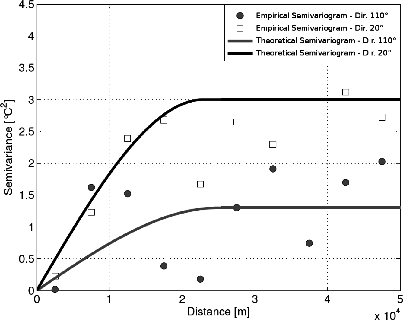
For the OK method, the possible presence of anisotropic patterns was explored, despite the limited number of available stations. Indeed, the experimental semivariogram is a function of both distance and direction, so it can account for anisotropic patterns revealed by the data. In particular, it was observed that the sill varies along different directions, determining the phenomenon known as zonal anisotropy [35]. The zonal direction, i.e., the direction of maximum variability, was found at 20 degrees measured clockwise from the north (Figure 2).

The theoretical zonal anisotropic semivariogram was operationally modeled by summing an isotropic semivariogram, given by the first term, to a geometrical anisotropic semivariogram with a small anisotropy ratio (according to the procedure suggested for the GSTAT software; see Pebesma and Wesseling [43]). With regard to the average annual temperature data, the theoretical semivariogram, calibrated with a manual procedure, assumes the following form:

$$\mathrm{\gamma }=1.3Sph(25000)+1.7Gau(2.5\times {10}^4,110,0.0001)$$

(22)

In particular, 1.25 °C² is the partial sill of the theoretical semivariogram at the principal direction (called c₁, in GSTAT nomenclature); 1.75 °C² is the value that was summed to c₁ to obtain partial sill in the zonal direction (called c₂); 25, 000 m is the maximum range of the variogram model (called a₁), 1.25 × 10⁴ m is the maximum range amplified (called a₂); 110 degrees is the angle for the principal direction (called p); 0.0001 is the range ratio (i.e., the ratio between the minor range and the maximum range, called s). It has been decided not to consider the nugget effect, because information about possible sensor errors was not available. Furthermore, data have been preprocessed and possible data anomalies checked. In order to model possible high variability in the short range, the spherical model (Sph), almost linear at its origin, has been selected. The additive model used for the anisotropic formulation is the Gaussian model (Gau), varying very smoothly at the origin and allowing for a gradual development with respect to the principal direction semivariogram.

Performance indices (RMSE, MBE and CC) of OK are comparable to those obtained with the best IDW trial, but worse than those obtained with RBF, which can be definitely considered the best method, among the univariate, in terms of accuracy, bias and correlation for annual temperature field.

3.2. Variable Aided Methods

The results of the application of VAI algorithms for the spatial interpolation are reported in

Table 2. Comparison of indices of interpolation goodness of the variable-aided (VAI) interpolation methods applied to mean annual temperature.

Methods			RMSE [°C]	MBE [°C]	MAE [°C]	CC
LR	OLS	z = f(q)	0.4886	−0.0014	0.376	0.9598
		log(z) = f(q)	0.5369	−0.0039	0.4196	0.9445
		sqrt(z) = f(q)	0.5113	−0.0028	0.3954	0.9535
	ROB	z = f(q)	0.4909	−0.0098	0.3784	0.9598
		log(z) = f(q)	0.5423	−0.0058	0.4218	0.9452
		sqrt(z) = f(q)	0.5165	−0.0012	0.4	0.9537
MLR	SW	Ts = 18.68 – 0.0057 q – 8 × 10−6 Ds	0.501	0.0159	0.3617	0.9572
GWR		N = 5	0.7363	0.1176	0.5366	0.9113
		N = 10	0.5376	−0.0064	0.4081	0.9515
		N = 15	0.5585	−0.0026	0.4509	0.9469
		N = 20	0.4996	0.028	0.3939	0.9588
		N = 25	0.5131	0.0298	0.4132	0.9562
		N = 30	0.5176	0.0762	0.4179	0.9592
		N = 35	0.5068	0.0688	0.4034	0.9595
ANN		MLP 3 - 3 - 1	0.4464	−0.0153	0.3478	0.9663
		MLP 3 - 4 - 1	0.4193	−0.0158	0.3161	0.9703
		MLP 3 - 6 - 1	0.4849	−0.0186	0.3455	0.9607
		MLP 3 - 8 - 1	0.51	−0.005	0.3689	0.9556
		MLP 3 - 10 - 1	0.5833	−0.0816	0.4592	0.9435
		MLP 3 - 15 - 1	0.6304	−0.127	0.4984	0.9348
RK		GWR: N = 20	0.3592	−0.0582	0.274	0.9692
		LR-OLS; z = f(q)	0.33	−0.0124	0.1098	0.9797
		ANN-MLP 3 - 4 - 1	0.3655	0.015	0.2505	0.9779
		ML	0.347	0.0171	0.2677	0.9676

. The ordinary least squares (OLS) and the robust (ROB) regression methods were used for regression coefficient estimation. The first of these provides the best results in terms of both MBE and RMSE, but the differences in terms of accuracy and unbiasedness between the two methods are negligible, suggesting the absence of outliers in the temperature dataset.

The second VAI method (GWR) was applied adopting a searching strategy based on the number of closest points to be considered in the estimate. The best performance, in terms of accuracy and correlation, was obtained for N greater than 20, while, in terms of bias, for N equal to 15. In general, the best results of GWR are comparable to those of LR.

The third VAI method is the multiple linear regression (MLR), which estimates temperature by exploiting its dependence on geographic and physiographic features. Once the indices listed in Section 2.4 were derived, a stepwise regression procedure was applied to the training set to build the model that links the mean annual temperature to the morphological parameters. This involves the generation of multiple regression models of increasing complexity, according to the number of independent variables considered. These models have been compared and evaluated using the coefficient of determination R², the RMSE and the test on coefficients significance of T stat, given by the ratio between R² and the standard error. The best results in terms of RMSE and R² were obtained by the use of q (elevation), L and D_s as independent variables, but the value of T stat for L suggests neglecting the latter variable. Finally, the best model for mean annual temperature is only based on elevation q (m a.s.l.) and the geometric mean of the distance from the sea in the eight cardinal directions D_s (m), as follows:

$${\widehat{T}}_a=18.68-0.0057q+8\times {10}^{-6}{D}_s$$

(23)

The performance indices provided by this method are satisfactory, both in terms of RMSE (lower than for GWR and LR) and for MBE. Moreover, the CC value, equal to 0.96, confirms an excellent agreement between estimates and observations.

3.2.1. Artificial Neural Networks

The results of the application of ANNs are reported together with those of VAI methods in Table 2. The ANN was trained by the scaled conjugate gradient algorithm, and the initial weights were randomly extracted from a standardized normal distribution. The learning rate decreased exponentially from 0.01 to 0.0001. Six network architectures, having different numbers of neurons in the hidden layer, were compared, and on the basis of RMSE and MBE performances, the best resulted in being a network with one hidden layer, having four neurons with a hyperbolic tangent activation function (MLP 3-4-1). In terms of RMSE, the ANN performances overcame those of LR, MLR and GWR, while the MBE value was slightly worse than that provided by MLP 3-8-1. Moreover, the correlation coefficient between estimated and measured data for the validation set was equal to 0.97, confirming an excellent agreement within the validation dataset. This confirms the ANN as a suitable algorithm to estimate nonlinear processes, such as temperature, as well as other hydroclimatic variables.

3.2.2. Residual Kriging

The correlation coefficient between measured data and residuals provided by LR, equal to −0.44, highlights that not all of the spatial data correlations can be explained by LR methods, and a similar observation can be done for the MLR and MLP with four neurons in the hidden layer, whose correlation coefficient between measured data and residuals is equal to −0.4 and −0.35, respectively. This highlights that the residuals obtained by VAI methods still show a spatial correlation that can be exploited to improve the variable estimation. Starting from these considerations, residual kriging (RK) was used as a further VAI method by applying OK to the residuals derived from LR, MLR, GWR and ANN (MLP 3-4-1). In this case, an isotropic behavior in the residuals coming from the four different methods was observed when deriving the experimental semivariograms. As previously explained, the estimated values of residuals were added to the LR, MLR, GWR and ANN, respectively. In terms of accuracy and correlation, the performances of these methods are better than the univariate method and the other VAI methods (Table 2), while the bias is comparable to that of the other VAI methods. The best method, in terms of RMSE, MBE and CC, appears to be the RK-LR (with OLS).

3.3. Monthly Analysis

The interpolation methods with the best performance, described for the case of average annual temperature data, have been also applied to mean monthly temperature. Particular attention was paid to the estimation of the semivariograms of both the average monthly data (i.e., OK) and the residuals coming from the use of four VAI and ANN methods (i.e., LR, MLR, GWR and MLP 3-4-1). In this regard, the presence of a zonal anisotropy was observed in mean monthly data for all months with the exception of the summer months (JJA). Moreover, for the mean monthly temperature, another method has been taken into account: the Fourier series with the estimation of parameters by an MLR method. In particular, the first attempt to reconstruct the zero-mean temperature regime was made with a one-harmonic (N = 1) Fourier series (F1H), with τ₁ = 12 months. The parameters A₁ and ϕ₁ of the Fourier equation were then correlated with the geographical and physiographic descriptors (q (m a.s.l.), L (hexadecimal degrees), D_s (m), A_s (m⁻¹), C), defined before, using the stepwise procedure to check the presence of any statistically significant relationship. Results of this multi-regressive analysis point out that the most efficient models found for amplitude A₁ and phase ϕ₁ are:

$$A_1=-1.1\times {10}^{-3}q+0.3024L+1.16\times {10}^{-4}{D}_s-18.69$$

(24)

$${\mathrm{\varphi }}_1=-5.88\times {10}^{-5}q+7.59\times {10}^{-7}{D}_s-0.8385$$

(25)

Despite fair model results, significant errors occur in correspondence with the pairs of consecutive months with either the lowest or highest temperature (December and January, and July and August, respectively). In order to improve the temperature cycle reproduction and to avoid this problem, a second Fourier wave (F2H) with τ₂ = 6 months was used. In this case, least-squares regressions of the four parameters for all stations produced estimates of A₁ and ϕ₁ almost identical to those obtained considering only one harmonic. The analysis of the second harmonic parameters showed that A₂ and ϕ₂ can be considered constant in space, with an average value of 0.12 and 2.03, respectively.

Finally, monthly mean temperatures can be reconstructed using the following combined model:

$$\widehat{T}(j)=T_a+t(j)=T_a+A_1\mathit{cos}\left(\frac{2\mathrm{\pi }}{12}j+{\mathrm{\varphi }}_1\right)+A_2\mathit{cos}\left(\frac{4\mathrm{\pi }}{12}j+2{\mathrm{\varphi }}_2\right)$$

(26)

where T_a is the mean annual temperature, obtained with one of the above-mentioned methods. In this application, T_a is the estimated mean annual temperature obtained by RK-ANN (MLP 3-4-1).

In

Table 3. Results of monthly analysis; each box reports the interpolation model leading to the best result for each index, and the corresponding value of the index.

Month	RMSE [°C]	MBE [°C]	MAE [°C]	CC
January	F2H	RK-OLS	RK-GWR	RK-GWR
	0.39	0.005	0.29	0.99
February	RK-OLS	RK-GWR	RK-GWR	F2H
	0.19	−0.004	0.25	0.99
March	F2H	RK-GWR	RK-GWR	F2H
	0.27	0.000	0.25	0.99
April	RK-MLP	MLP	RK-OLS	F2H
	0.41	0.002	0.27	0.99
May	RK-OLS	RK-OLS	RK-OLS	RK-OLS
	0.26	0.027	0.28	0.96
June	F1H	MLP	F2H	F2H
	0.31	0.027	0.26	0.99
July	RK-GWR	MLP	RK-OLS	F2H
	0.44	−0.002	0.32	0.99
August	RK-OLS	LR	RK-OLS	RK-OLS
	0.46	0.008	0.33	0.94
September	FH2	RK-GWR	F2H	RK-OLS
	0.19	−0.023	0.16	0.96
October	F2H	RK-OLS	RK-OLS	F2H
	0.44	0.019	0.27	0.99
November	F2H	RK-OLS	RK-MLP	RK-MLP
	0.37	−0.006	0.28	0.98
December	F2H	RK-OLS	F2H	F2H
	0.32	−0.004	0.25	0.99

, an overview of the results is shown for monthly mean temperature. The best method is given for each month together with the corresponding value of the relative statistical indices. For RMSE values, the best results were always obtained with a VAI method. In particular, in seven of the 12 months, the lowest value of RMSE was achieved using the two-step VAI method, i.e., the Fourier series with the estimation of parameters by an MLR approach (F2H). For the other five months, the lowest value of RMSE was given by two-step VAI methods (RK-OLS, RK-MLP, RK-GWR). Differently from what was obtained at the annual scale, the best results in terms of unbiasedness were achieved with the VAI methods (direct application or two-step). Therefore, on the basis of these considerations, the F2H was chosen as the interpolator to be used to create the mean monthly air temperature maps.

4. Discussion and Application of the Best Interpolation Method

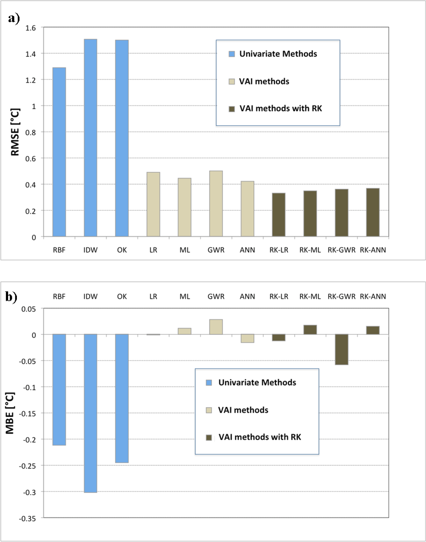
The performances of the best methods at the annual scale, respectively in terms of RMSE and MBE, for both univariate and VAI methods are shown in Figure 3. RBF with N = 30 can be considered the best univariate method. IDW skill has the worst performances, yielding higher RMSE and MBE than other univariate methods, while OK has intermediate skills between IDW and RBF. However, all univariate methods are very biased, providing a systematic underestimation of temperature. In order to improve the performance, it is necessary to switch from univariate methods to the VAI ones, by introducing the elevation information, in the case of LR, GWR and ANN methods, or by introducing elevation and physiographic information, in the case of ML. Indeed, from a comparison of the performance indices in Tables 1 and 2, it can be observed that with the VAI methods, RMSE and MBE subside dramatically. In particular, while the LR is characterized by the lowest bias, but relatively high RMSE, methods, such as GWR, ANN and MLR, provide good results, with acceptable values of RMSE and with MBEs substantially higher than those obtained with LR. The best results, in terms of RMSE, are achieved by RK and, in particular, RK-LR, which gives the lowest RMSE and the highest CC. In general, the application of OK to the residuals resulting from any VAI method remarkably decreases the RMSE of the underlying VAI method, as can be observed also in Figure 3a. However, taking into account the values of the two indices, RMSE and MBE, at the same time, one can note that a simple method such as LR (ROB), characterized by an RMSE value 36% higher than for RK -LR, has an improvement, in terms of MBE, of about 90% if compared to the MBE value of RK-LR. The values of CC are comparable.

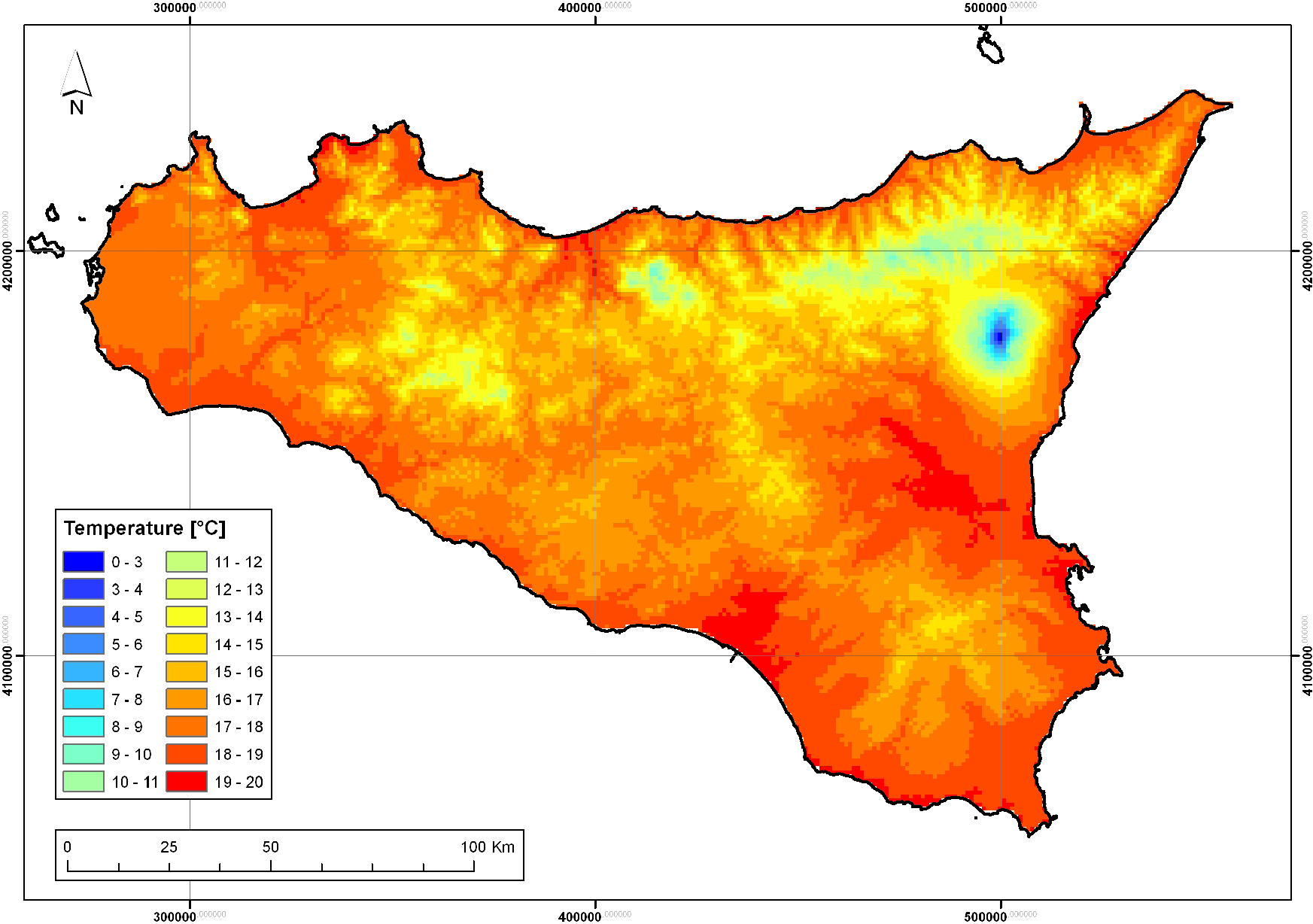
On the basis of the previous considerations, both LR and RK-LR (with OLS) could be chosen as the best method and used for spatial interpolation of the mean annual temperature. The mean annual temperature map obtained by RK-LR is shown in Figure 4.

Regarding the analysis at the monthly scale, the spatial variation of the cyclical temperature pattern was found to be linearly dependent on the distance from the sea and latitude, in addition to elevation. The parameters of the two-harmonic Fourier series reproducing the temperature regime have been related to the above-mentioned physiographic predictors through a linear multivariate model, without the need to build 12 different models, one for each month. The results of the regression analysis clearly show that the amplitude and phase of the temperature cycle are affected by elevation and distance from the sea and also by latitude (only amplitude). Different spatial dependencies had been found by Claps et al. [16], who applied the procedure over the entire Italian territory, pointing out another advantage of this method: it allows one to easily assess the influence of the various parameters at different spatial scales.

Retrieved standard deviation (SD) and correlation coefficient (CC) values were used as polar coordinates on the Taylor diagram (Figure 5), which displays the relationships of these values with the centered pattern error component, therefore not considering the bias component. OK and IDW have very similar performances, while RBF shows better performances in terms of centered root-mean-square difference (RMSD). VAI methods are clustered, with definitely better skill than the univariate methods thanks to the higher CC and SD values, at least in two of the three univariate methods, closer to those of observations. Standard deviation values for the two groups seem related to their mean CC; moreover, it seems that a minimum RMSD level related to the corresponding mean CC is reached by both groups. This effect could be due to the calibration operations performed for each interpolation method by means of parameter selection.

5. Conclusions

The availability of climatic maps, a key issue for agricultural, hydrological and environmental management, has increased in the last few decades thanks to the spread of new and efficient spatial interpolation techniques and GIS tools. Due to the relative abundance of methods, many algorithms are currently applied, and investigations continue, aiming at the definition of the “best” method for each single climatic variable. This study calibrated and compared nine different methods for spatial interpolation of temperature at the annual and monthly scale over Sicily, a Mediterranean island and a region with complex topography.

Different families of methods were considered: univariate, multivariate, artificial neural networks, a model to describe the cyclical nature of monthly temperature and a two-step application of methods. This comparison highlighted that among the univariate methods, the best performance, in terms of accuracy and unbiasedness, was obtained with RBF, performing better than the geostatistical method OK. Indeed, although RBF is a simple method that does not take into account any external variable, it yielded quite low RMSE (1.28 °C) and bias (−0.21 °C).

Several methods were implemented that take into account elevation and other geographic and physiographic parameters, from the simpler deterministic methods (i.e., linear simple or multiple regression and geographically-weighted regression) to more sophisticated ones. In particular, a reduction of 74.4% of the RMSE is possible using one of the best variable-aided interpolation methods instead of the best univariate one. The introduction of geographic and physiographic variables improves the interpolation performances, highlighting the importance of this information for modeling temperature in a complex morphology region, such as Sicily. On the whole, the best results, for mean annual temperature were achieved by both the application of a geostatistical method to the result of a deterministic one (the RK based on LR) and by the use of a simple method, such as LR.

At the monthly scale, the best results in terms of accuracy and unbiasedness have been obtained by the F2H application, which also takes into account the contribution of a second six-month harmonic. These results open the way for the implementation of a very efficient two-step interpolation technique for monthly temperatures resulting from the interpolation at the annual scale, carried out with linear regression and ordinary kriging of residuals, and the eventual monthly downscaling of annual results by the Fourier series method.

Finally, the results lead to the elaboration of reliable temperature maps, which can significantly contribute to the proper application of hydrological modeling, e.g., for water management, for the monitoring and management of the hydrogeological risk and for the climatological characterization of the territory.

References

- Krajewski, W.; Kruger, A.; Smith, J.; Lawrence, R.; Gunyon, C.; Goska, R.; Seo, B.; Domaszczynski, P.; Baeck, M.; Ramamurthy, M.; et al. Towards better utilization of NEXRAD data in hydrology: An overview of Hydro-NEXRAD. J. Hydroinform. 2011, 13, 255–266. [Google Scholar]
- Liuzzo, L.; Noto, L.; Vivoni, E.; la Loggia, G. Basin-scale water resources assessment in Oklahoma under synthetic climate change scenarios using a fully distributed hydrologic model. J. Hydrol. Eng. 2010, 15, 107–122. [Google Scholar]
- Burrough, P.; McDonnell, R.; McDonnell, R. Principles of Geographical Information Systems; Oxford University Press: Oxford, UK, 1998; Volume 333. [Google Scholar]
- Vicente Serrano, S.M.; Sánchez, S.; Cuadrat, J.M. Comparative analysis of interpolation methods in the middle Ebro Valley (Spain): Application to annual precipitation and temperature. Clim. Res. 2003, 24, 161–180. [Google Scholar]
- Hofstra, N.; Haylock, M.; New, M.; Jones, P.; Frei, C. Comparison of six methods for the interpolation of daily, European climate data. J. Geophys. Res. Atmos. 2008, 113. [Google Scholar] [CrossRef]
- Serbin, S.P.; Kucharik, C.J. Spatiotemporal mapping of temperature and precipitation for the development of a multidecadal climatic dataset for Wisconsin. J. Appl. Meteorol. Climatol. 2009, 48, 742–757. [Google Scholar]
- Li, J.; Heap, A.D. A review of comparative studies of spatial interpolation methods in environmental sciences: Performance and impact factors. Ecol. Inform. 2011, 6, 228–241. [Google Scholar]
- Willmott, C.; Robeson, S.; Feddema, J. Estimating continental and terrestrial precipitation averages from rain-gauge networks. Int. J. Climatol. 1994, 14, 403–414. [Google Scholar]
- Li, J.; Heap, A.D. Spatial interpolation methods applied in the environmental sciences: A review. Environ. Model. Softw. 2014, 53, 173–189. [Google Scholar]
- Price, D.; McKenney, D.; Nalder, I.; Hutchinson, M.; Kesteven, J. A comparison of two statistical methods for spatial interpolation of Canadian monthly mean climate data. Agric. For. Meteorol. 2000, 101, 81–94. [Google Scholar]
- Daly, C.; Gibson, W.; Taylor, G.; Johnson, G.; Pasteris, P. A knowledge-based approach to the statistical mapping of climate. Clim. Res. 2002, 22, 99–113. [Google Scholar]
- Taskinen, A.; Sirviö, H.; Vehviläinen, B. Interpolation of daily temperature in Finland. Nord. Hydrol. 2003, 34, 413–426. [Google Scholar]
- Teegavarapu, R.S.V. Estimation of missing precipitation records integrating surface interpolation techniques and spatio-temporal association rules. J. Hydroinform. 2009, 11, 133–146. [Google Scholar]
- Tobin, C.; Nicotina, L.; Parlange, M.B.; Berne, A.; Rinaldo, A. Improved interpolation of meteorological forcings for hydrologic applications in a Swiss Alpine region. J. Hydrol. 2011, 401, 77–89. [Google Scholar]
- Naoum, S.; Tsanis, I.K. A multiple linear regression GIS module using spatial variables to model orographic rainfall. J. Hydroinform. 2004, 6, 39–56. [Google Scholar]
- Claps, P.; Giordano, P.; Laguardia, G. Spatial distribution of the average air temperatures in Italy: Quantitative analysis. J. Hydrol. Eng. 2008, 13, 242–249. [Google Scholar]
- Arnone, E.; Francipane, A.; Noto, L.V.; Scarbaci, A.; la Loggia, G. Strategies investigation in using artificial neural network for landslide susceptibility mapping: Application to a Sicilian catchment. J. Hydroinform. 2014, 16, 502–515. [Google Scholar]
- Hettiarachchi, P.; Hall, M.; Minns, A. The extrapolation of artificial neural networks for the modeling of rainfall-runoff relationships. J. Hydroinform. 2005, 7, 291–296. [Google Scholar]
- Rigol, J.; Jarvis, C.; Stuart, N. Artificial neural networks as a tool for spatial interpolation. Int. J. Geogr. Inf. Sci. 2001, 15, 323–343. [Google Scholar]
- Coulibaly, P.; Evora, N. Comparison of neural network methods for infilling missing daily weather records. J. Hydrol. 2007, 34, 27–41. [Google Scholar]
- Goovaerts, P. Using elevation to aid the geostatistical mapping of rainfall erosivity. Catena 1999, 34, 227–242. [Google Scholar]
- Di Piazza, A.; lo Conti, F.; Noto, L.; Viola, F.; la Loggia, G. Comparative analysis of different techniques for spatial interpolation of rainfall data to create a serially complete monthly time series of precipitation for Sicily, Italy. Int. J. Appl. Earth Obs. Geoinf. 2011, 13, 396–408. [Google Scholar]
- Karavitis, C.A.; Alexandris, S.; Tsesmelis, D.E.; Athanasopoulos, G. Application of the standardized precipitation index (SPI) in Greece. Water 2011, 3, 787–805. [Google Scholar]
- Haining, R.P.; Kerry, R.; Oliver, M.A. Geography, spatial data analysis, and geostatistics: An overview. Geogr. Anal. 2010, 42, 7–31. [Google Scholar]
- Hudson, G.; Wackernagel, H. Mapping temperature using kriging with external drift: Theory and an example from Scotland. Int. J. Climatol. 1994, 14, 77–91. [Google Scholar]
- Demyanov, V.; Kanevsky, M.; Chernov, S.; Savelieva, E.; Timonin, V. Neural network residual kriging application for climatic data. J. Geogr. Inf. Decis. Anal. 1998, 2, 215–232. [Google Scholar]
- Antonic, O.; Krizan, J. Spatio-temporal interpolation of climatic variables over large region of complex terrain using neural networks. Ecol. Model. 2001, 138, 255–263. [Google Scholar]
- Willmott, C.; Matsuura, K. Smart interpolation of annually averaged air temperature in the United States. J. Appl. Meteorol. 1995, 34, 2577–2586. [Google Scholar]
- Wu, T.; Li, Y. Spatial interpolation of temperature in the United States using residual kriging. Appl. Geogr. 2013, 44, 112–120. [Google Scholar]
- Prudhomme, C.; Reed, D. Mapping extreme rainfall in a mountainous region using geostatistical techniques: A case study in Scotland. Int. J. Climatol. 1999, 19, 1337–1356. [Google Scholar]
- Faulkner, D.; Prudhomme, C. Mapping an index of extreme rainfall across the UK. Hydrol. Earth Syst. Sci. 1998, 2, 183–194. [Google Scholar]
- Bishop, C.M. Neural Networks for Pattern Recognition; Clarendon Press: Oxford, UK, 1995. [Google Scholar]
- Isaaks, E.; Srivastava, R. An Introduction to Applied Geostatistics; Oxford University Press: Oxford, UK, 1990. [Google Scholar]
- Kitanidis, P. Introduction to Geostatistics: Applications in Hydrogeology; Cambridge University Press: Cambridge, UK, 1997. [Google Scholar]
- Goovaerts, P. Geostatistics for Natural Resources Evaluation; Oxford University Press: Oxford, UK, 1997. [Google Scholar]
- Andrews, D.F. A Robust Method for Multiple Linear Regression. Technometrics 1974, 16, 523–531. [Google Scholar]
- Brunsdon, C.; McClatchey, J.; Unwin, D. Spatial variations in the average rainfall-altitude relationship in Great Britain: An approach using geographically weighted regression. Int. J. Climatol. 2001, 21, 455–466. [Google Scholar]
- Fotheringham, S.; Brunsdon, C.; Charlton, M. Geographically Weighted Regression: The Analysis of Spatially Varying Relationships; Wiley: Chichester, UK, 2002. [Google Scholar]
- Govindaraju, R., Rao, A., Eds.; Artificial Neural Networks in Hydrology; Kluwer Academic Publishers: Dordrecht, The Netherlands, 2000.
- Bahrami, J.; Kavianpour, M.R.; Abdi, M.S.; Telvari, A.; Abbaspour, K.; Rouzkhash, B. A comparison between artificial neural network method and nonlinear regression method to estimate the missing hydrometric data. J. Hydroinform. 2011, 13, 245–254. [Google Scholar]
- Goovaerts, P. Geostatistical approaches for incorporating elevation into the spatial interpolation of rainfall. J. Hydrol. 2000, 228, 113–129. [Google Scholar]
- Taylor, K.E. Summarizing multiple aspects of model performance in a single diagram. J. Geophys. Res. 2001, 106, 7183–7192. [Google Scholar]
- Pebesma, E.; Wesseling, C. Gstat: A program for geostatistical modeling, prediction and simulation. Comput. Geosci. 1998, 24, 17–31. [Google Scholar]