
Quantification of Water and Salt Exchanges in a Tidal Estuary


1
Dynamic Solutions International LLC, Edmonds, WA 98020, USA
2
Department of Civil Engineering, Auburn University, Auburn, AL 36849-5337, USA
*
Author to whom correspondence should be addressed.
Water 2015, 7(5), 1769-1791; https://doi.org/10.3390/w7051769
Submission received: 28 January 2015
/
Revised: 6 April 2015
/
Accepted: 20 April 2015
/
Published: 24 April 2015
(This article belongs to the Special Issue Water Quality Control and Management)
Abstract
:A calibrated three-dimensional hydrodynamic model was applied to study subtidal water and salt exchanges at various cross sections of the Perdido Bay and Wolf Bay system using the Eulerian decomposition method from 6 September 2008 to 13 July 2009. Salinity, velocity, and water levels at each cross section were extracted from the model output to compute flow rates and salt fluxes. Eulerian analysis concluded that salt fluxes (exchanges) at the Perdido Pass and Dolphin Pass cross sections were dominated by tidal oscillatory transport FT, whereas shear dispersive transport FE (shear dispersion due to vertical and lateral shear transport) was dominant at the Perdido Pass complex, the Wolf-Perdido canal, and the lower Perdido Bay cross sections. The flow rate QF and total salt transport rate FS showed distinct variation in response to complex interactions between discharges from upstream rivers and tidal boundaries. QF and FS ranged from −619 m3·s−1 (seaward) to 179 m3·s−1 (landward) and −13,480–6289 kg·s−1 at Perdido Pass when river discharges ranged 11.0–762.5 m3·s−1 in the 2008–2009 simulation period.
1. Introduction
Estuaries are extremely productive regions due to the high flux of nutrients from the land and serve as breeding and nursery grounds for many species [1]. The impact of anthropogenic activity on the estuarine environment is a frequent concern because many major cities are located next to estuaries [2]. Neither estuaries nor oceans are capable of assimilating pollutants indefinitely; therefore, the increasing environmental concerns require the proper regulation and management of pollutant released in coastal zone [3]. To study the ecology of tidal estuaries, the exchanges of fresh and salt water are important not only in determining the characteristics of the environment [4] but also for water quality control and management. The circulation and salinity distribution patterns in an estuary depend on several factors such as river inflow pushing seaward, denser ocean water sliding landward, and tidal currents stirring and mixing the two [5]. The “exchange flow” or “gravitational circulation”, which is characterized by deep inflow (denser salt intrusion in bottom layers) and shallow outflow (seaward freshwater flow in surface layers) through a cross section, dominates circulation in many estuaries [5]. Mean circulation and the circulation with frequencies lower than the semidiurnal and diurnal tides are often collectively called the residual circulation [6,7] because they are the residual of a time average over the principal periods.
The magnitude and direction of velocity and salinity determine the salt transport, which may affect inlet design of water supply in an estuary. The net outflow continually removes salt from the estuary whereas salt is brought back into the estuary by the “estuarine salt transport”, i.e., the vertical and lateral variations of tidally-averaged velocity and salinity, and “tidal dispersion”, i.e., the tidal correlations of velocity and salinity [8]. The magnitude of salt transport and the processes that contribute to it depend on the bathymetry of the estuary and on the strength of the physical forcing (e.g., tides, freshwater inflows, wind, etc.). In strongly stratified estuaries, salt transport is predominantly due to advection by the net landward flow and the estuarine salt transport [9]. However, in relatively well-mixed estuaries that are weakly stratified, tidal dispersion plays a larger role in the salt balance [10]. The stratification of partially stratified estuaries varies between these extremes. To understand characteristics of the time-variant estuary fluxes at different cross sections, these fluxes are further divided into two components: a subtidal component, which is a result of residual velocity and salinity; and an oscillatory tidal component, which is related to correlations in velocity and salinity at tidal time scales [11,12].
Several methods of determining the flow and salt exchange in estuaries have been formulated and verified successfully by various scientists [3,5,13,14,15,16,17,18]. Ketchum [4] developed an empirical method which computes the average distribution of fresh and salt water in an estuary and explains the exchange across various cross sections resulting from tidal oscillations. Bilgili et al. [3] used a Lagrangian particle tracking method embedded within a two-dimensional finite element model to study the transport and ocean-estuary exchange processes in the relatively well-mixed Great Bay Estuarine System in New Hampshire, USA. Using the Regional Ocean Modeling System, Chen et al. [18] used isohaline coordinate analysis to study the exchange flow characteristics in two different estuaries: the long (with respect to tidal excursion) Hudson River and the short Merrimack River.
This study used a previously calibrated Environmental Fluid Dynamic Code (EFDC) model [19] to investigate the flow and salt exchange across various cross sections to understand the underlying transport phenomena and mechanisms in the Perdido Bay and Wolf Bay (PBWB) system (Figure 1) including additional calibration on filtered water surface elevation (Figure 2). Xia et al. [20] used the EFDC model to understand distributions and dynamics of salinity and dissolved oxygen at Perdido Bay and the Gulf of Mexico. Xia et al. [21] studied the responses of estuarine plumes near the shoreline of the Gulf of Mexico under different wind conditions. They found that outflow from the estuary to the Gulf were strongest under northerly winds and could be stopped by southerly winds. Xia et al. [21] used the EFDC model to understand plume dynamics in Perdido Bay using idealized sensitivity experiments to examine the influence of wind stress on the three-dimensional plume signatures.
Figure 1.
Environmental Fluid Dynamic Code (EFDC) model domain for Wolf Bay and Perdido Bay connected to the Gulf of Mexico through Perdido Pass, to eastern Big Lagoon through Dolphin Pass, and to western Mobile Bay through the Gulf Intracoastal Waterway (GIWW), showing the colored contours of bottom elevation and cross sections (A–A, B–B, C–C, D–D, and E–E) where water and salt fluxes were calculated. A centerline from Perdido Pass to Perdido River is represented using a series of dots for studying the salinity profile. White dashed lines refer to three cross sections used in Figure 3 and for discussion in the paper.
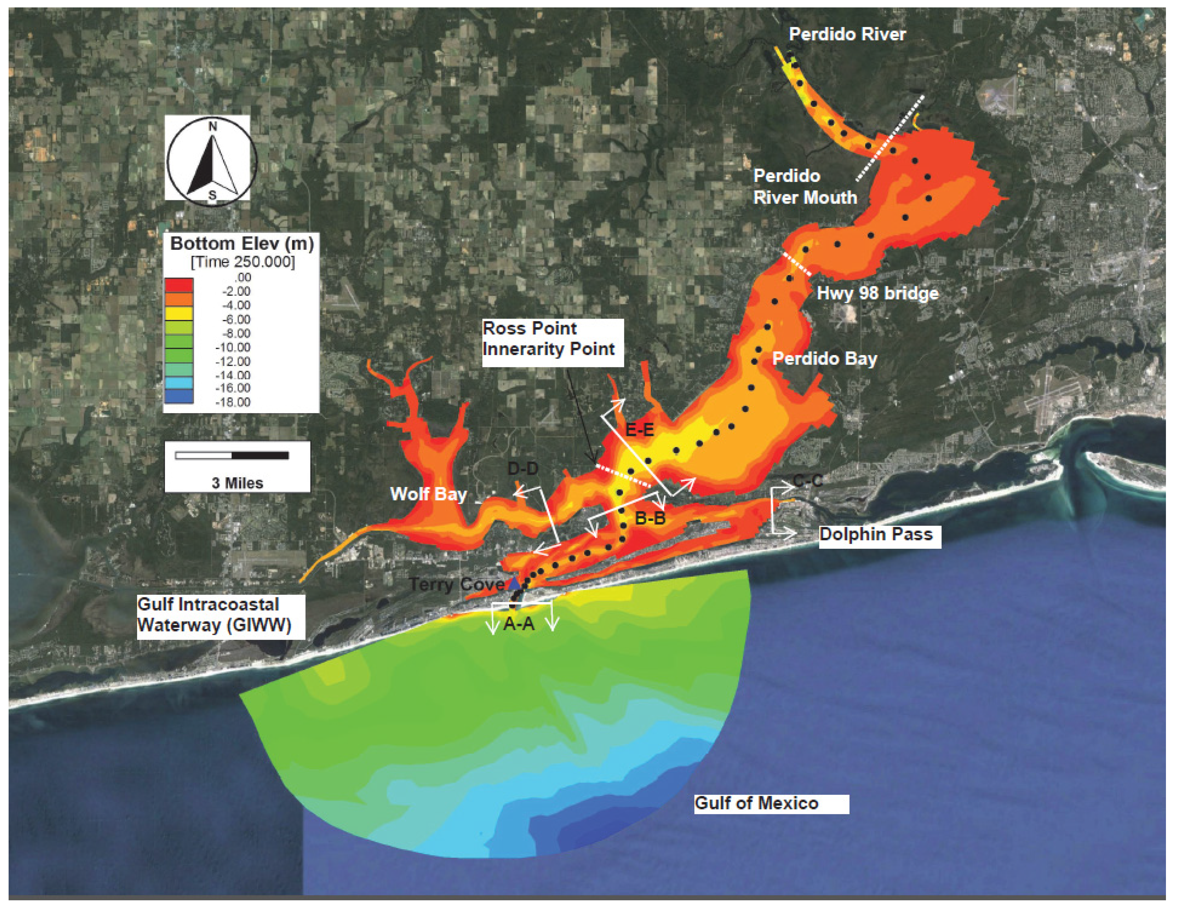
Devkota et al. [19] developed and calibrated an EFDC model for the PBWB system to understand the age of water in the system under different inflows from the rivers flowing into Wolf Bay and Perdido Bay. The model was calibrated from 6 September 2008 (Julian Day 250) to 13 July 2009 (Julian Day 560 starting from 1 January 2008). The PBWB system is connected to the Gulf of Mexico via three open boundaries (Figure 1): Perdido Pass on the south, Dolphin Pass—Connected to Big Lagoon and eventually to Pensacola Bay—On the East, and the Gulf Intracoastal Waterway (GIWW—Connected to the Mobile Bay and eventually to the Gulf of Mexico—To the West.
Figure 2.
Modeled and observed filtered water surface elevations at Terry Cove from 27 October 2008 (Julian Day 300) to 3 July 2009 (Julian Day 184).
Figure 2.
Modeled and observed filtered water surface elevations at Terry Cove from 27 October 2008 (Julian Day 300) to 3 July 2009 (Julian Day 184).
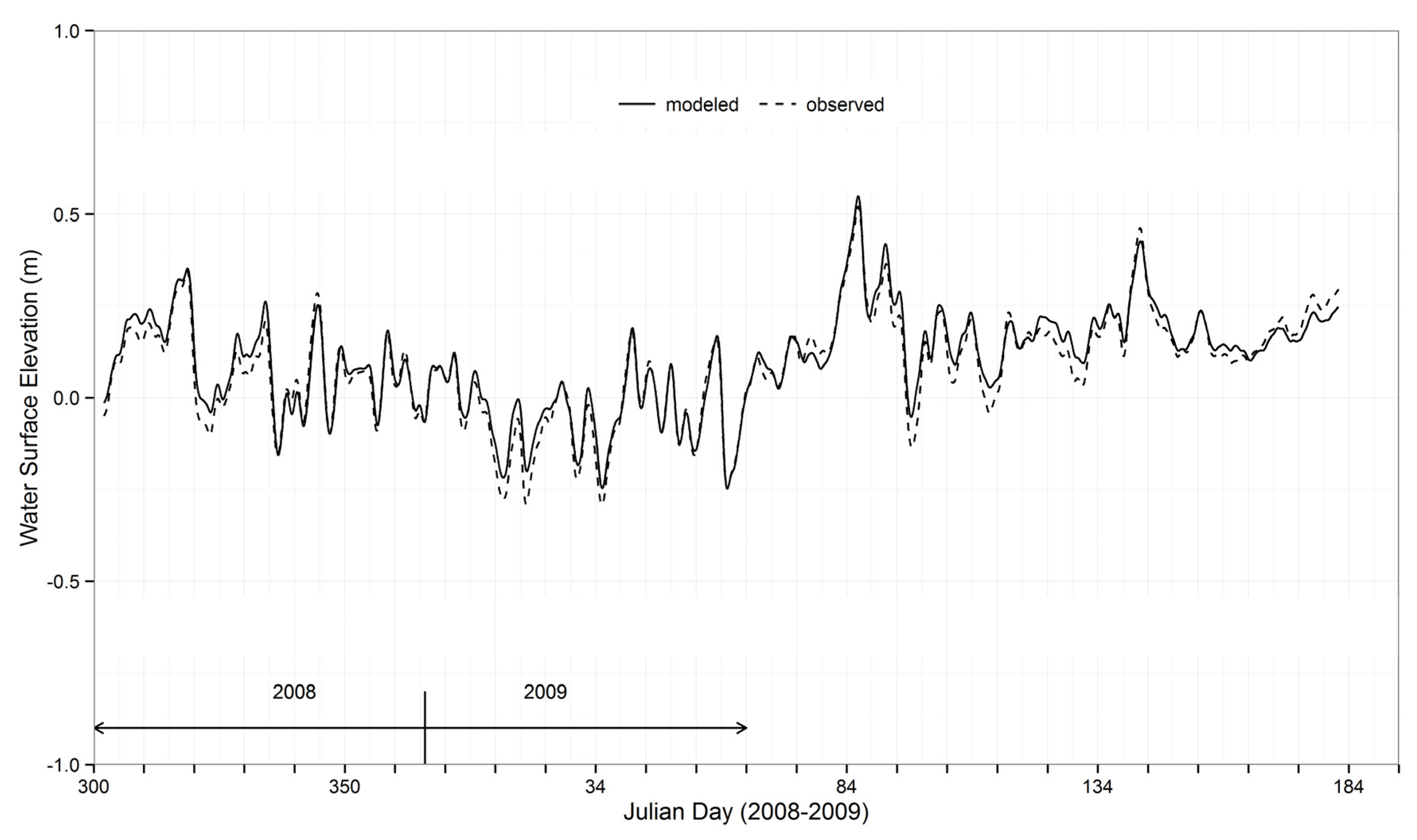
Figure 3.
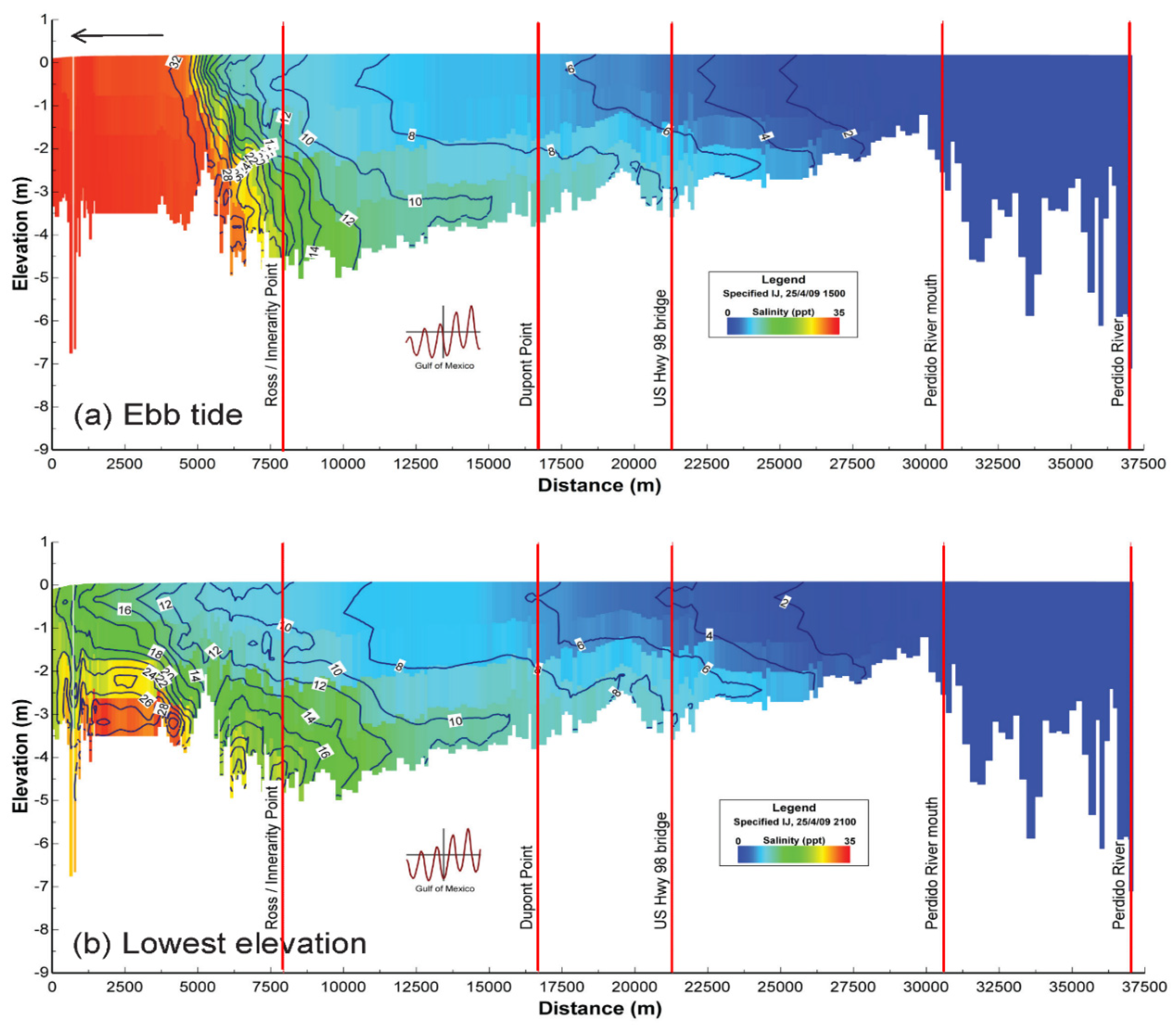
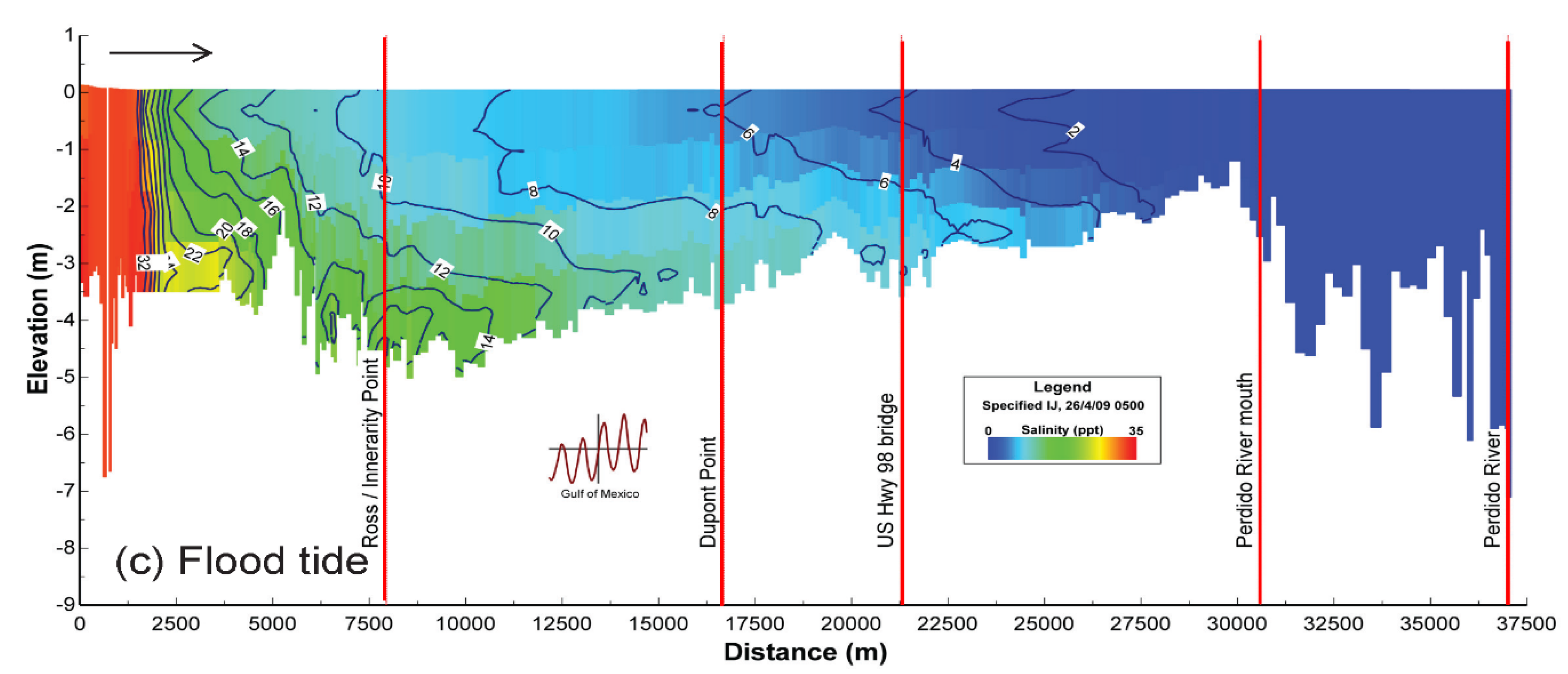
Simulated salinity profile contour plots through the centerline (Figure 1) from Perdido Pass to Perdido River during low flows from upstream under (a) ebb tide (15:00 25 April 2009) (b) the lowest water surface elevation (21:00 25 April 2009); and (c) flood tide (05:00 26 April 2009) at the Gulf of Mexico. Simulated salinity contour lines of 0–34 psu are shown in addition to colored contour maps.
Figure 3.
Simulated salinity profile contour plots through the centerline (Figure 1) from Perdido Pass to Perdido River during low flows from upstream under (a) ebb tide (15:00 25 April 2009) (b) the lowest water surface elevation (21:00 25 April 2009); and (c) flood tide (05:00 26 April 2009) at the Gulf of Mexico. Simulated salinity contour lines of 0–34 psu are shown in addition to colored contour maps.


In this study, we tried to answer the following three flow and salt exchange related questions: (1) How much salt is imported into Perdido Bay via Perdido Pass connection and how much fresh water is discharged from Perdido Bay to the Gulf of Mexico? (2) What factors are responsible for flow exchanges at different locations? (3) How much salt and water exchange takes place between Wolf Bay and Perdido Bay? In this paper we attempted to answer these questions by using the Eulerian salt decomposition method [5,22,23] with the calibrated EFDC model.
2. Materials and Methods
2.1. Study Area
The PBWB system (Figure 1) is a shallow to moderately deep inshore body of water [24] which has a length of 53.4 km and an average width of 4.2 km. Perdido Bay has an average depth of 2.6 m that increases gradually from the Perdido River mouth via lower Perdido Bay to the Gulf as indicated by elevation contours in Figure 1. The water depth in Perdido Bay tends to increase southward with the deepest parts of the estuary located at lower Perdido Bay, i.e., the cross section connecting Ross Point and Innerarity Point (Figure 1). The major freshwater inflows into Perdido Bay are Perdido River, Styx River, Elevenmile Creek, and Bayou Marcus [24]. The Perdido River combined with the Styx River provides more than 70% of the freshwater input into the estuary, and mean river discharge recorded at the U.S. Geological Survey (USGS) station at Barrineau Park, Florida is 21 m3·s−1 [19,21]. Perdido Pass is the primary pathway of salt water to Perdido Bay and controls salinity distributions in Perdido Bay [24]. The width of Perdido Pass ranges from 200 to 500 m, and depth is around 5 m. The diurnal tidal range at Perdido Pass is about 0.2 m [19,20]. Using a 48-hour Lanczos low-pass filter [25], the filtered water surface elevations at three open boundaries (GIWW, the Gulf of Mexico, and Big Lagoon, Table 1) have similar statistical characteristics during the calibration period. Wolf Bay is a sub-estuary of Perdido Bay with a connection to the GIWW (Figure 1) and has a contributing watershed area of 126 km2 [26]. The rivers that flow into Wolf Bay are Wolf Creek, Miflin Creek, Owens Bayou, Graham Bayou, and Hammock Creek, and combined flow into Wolf Bay ranged from 0.95–15.37 m3·s−1 with mean flow of 1.95 m3·s−1, which is very small in comparison to stream inflows to Perdido Bay (Table 1). Water in Wolf Bay flows through the GIWW into either Perdido Bay or Mobile Bay and ultimately into the Gulf of Mexico, and the flow directions depend on the magnitudes of wind and tide and the effect of the moon [27].

Table 1.
Statistical summary of river inflows into Wolf Bay and Perdido Bay and filtered water surface elevations at GIWW (Gulf Intracoastal Waterway, west boundary), the Gulf of Mexico (south boundary), and Big Lagoon (east boundary).
| Statistical Parameters | Discharges (m3·s−1) | Water Surface Elevation (m) | |||
|---|---|---|---|---|---|
| Wolf-Bay Rivers | Perdido-Bay Rivers | GIWW | Gulf of Mexico | Big Lagoon | |
| Minimum | 0.95 | 11.05 | −0.29 | −0.31 | −0.19 |
| Maximum | 15.37 | 762.45 | 0.58 | 0.56 | 0.54 |
| Mean | 1.95 | 38.81 | 0.10 | 0.10 | 0.14 |
| Standard Deviation | 1.97 | 66.05 | 0.14 | 0.15 | 0.17 |
| 1st Quartile | 1.11 | 14.61 | 0.019 | 0.01 | 0.00 |
| Median | 1.24 | 16.56 | 0.11 | 0.11 | 0.13 |
| 3rd Quartile | 1.74 | 32.83 | 0.20 | 0.20 | 0.25 |
2.2. Hydrodynamic Model
The calibrated EFDC model used for this study was developed by Devkota et al. [19] for the PBWB system, called the Perdido EFDC model with site-specific model inputs. EFDC is a three-dimensional hydrodynamic model framework that solves continuity, momentum, salt and heat transport equations. EFDC uses hydrostatic and Boussinesq approximations [28]. EFDC uses orthogonal curvilinear or Cartesian horizontal coordinates and a stretched sigma vertical coordinate. EFDC uses an internal-external mode splitting to numerically solve the momentum equations and solves internal and external modes at the same time step, but it solves the external mode semi-implicitly with respect to barotropic pressure gradient term in depth-averaged momentum equations [28,29,30]. The Mellor and Yamada level 2.5 turbulence closure scheme is implemented in the model [31,32]. EFDC simulates density and topographically-induced circulation, and tidal and wind-driven flows in an estuary in order to predict spatial and temporal distributions of salinity and temperature [28,33]. The Perdido EFDC model has a total of 4878 curvilinear horizontal grids and 4 uniform spacing vertical sigma layers. The grid sizes for the model ranged from 27 to 368 m and layer thicknesses ranged from 0.04 to 1.78 m in the PBWP system (not including the small portion of the Gulf). The details of the model configurations are presented by Devkota et al. [19].
Upstream boundaries for the Perdido EFDC model include inflows from the four rivers into Perdido Bay and the five streams into Wolf Bay [19]. During the simulation period (2008–2009) of this study, the mean and maximum inflow rates from the four rivers to Perdido Bay are 38.8 m3·s−1 and 762.45 m3·s−1 (Table 1), respectively. Overall, the discharges from upstream rivers during the calibration period 2008–2009 represent the typical flows, which resulted from typical rainfall in 2008 and 2009 (49.84 inches in dry 2008 and 91.40 inches in wet 2009). Wind speed plays an important role in Wolf Bay and Perdido Bay and ranged from 0 to 11.5 m·s−1 with an average value of 2.9 m·s−1 during the simulation period (2008–2009). The dominant winds during simulation periods are northerly, southerly and northeasterly winds. Southerly winds tend to push the water into the system via Perdido Pass whereas northerly and northeasterly winds push water out of the Perdido Bay. There are three locations in the model where the flow exchange takes place between the Perdido Wolf system and the Gulf of Mexico, Mobile Bay, and Pensacola Bay. The southern boundary “the Gulf of Mexico” (Figure 1) is the measured water surface elevation at Dauphin Island, a NOAA’s tides and currents station. Dolphin Pass is the location where the flow exchange between Perdido Bay and Pensacola Bay takes place via Big Lagoon. Measured time series of water surface elevation from the U.S. Army Corps of Engineers was used as the boundary condition at Dolphin Pass. The boundary condition at GIWW is the measured water surface elevation at the Gulf Shores NOAA’s tides and currents station to represent the flow exchange taking place between Wolf Bay and Mobile Bay (Figure 1).
2.3. Theoretical Formulation for Eulerian Decomposition Method
Eulerian decomposition approach can be used to study the salt flux in tidal rivers and estuaries and has been successfully used to predict the estuarine exchange [5,18,22,23]. In this approach, the tidally averaged (subtidal) salt flux (FS) through an estuarine cross section is decomposed into river flux (FR), exchange flow flux (FE), and tidal flux (FT). The equation to compute the subtidal salt flux FS (mass flow rate in kg·s−1) is given below based on Lerczak et al. [22]:
where 〈 〉 denotes a low-pass, subtidal temporal filter that produces tidally averaged/integrated component, u is the velocity in m·s−1 normal to the cross section as function of time and position on the cross section, s is the salinity in psu, and is the differential area of integration in m2. The subtidal volumetric flow rate (m3·s−1) through a cross-sectional area (A) is determined as
To simplify the calculation of salt fluxes through a cross section, the area is divided into a number of the cells along the section with constant differential areas dA along depth, but dA varies with time (expands and contracts tidally) and cell location (bottom elevation change). Velocity, salinity, and salt flux are also separated (decomposed) into three components. They are (a) tidally and cross-sectionally averaged; (b) tidally averaged and sectionally varying; and (c) tidally and sectionally varying remainder.
The tidally averaged properties are normalized using the tidally averaged, cross-sectional area [22]. Therefore, the tidally and sectionally averaged velocity ( ) and salinity ( ) are given by
Both and are negative when they are towards the ocean (seaward) because flow coming from the open boundary towards the model domain is considered positive. The tidally averaged and sectionally varying velocity () and salinity () are defined as
where is tidally averaged integration area. The exchange flow components ( and ) include the laterally and vertically varying part of the gravitational circulation [5]. The tidally varying and sectionally varying velocity () and salinity (), which vary with time and over the cross section, are defined by Lerczak et al. [22] as
The components and vary predominantly on tidal scales, while , , , and vary only on subtidal scales.
Finally, the subtidal salt flux can be decomposed into three components (river, exchange, and tidal) as follows:
In the above simplification, Lerczak et al. [22] have made use of the following properties to eliminate six of the nine terms;
The three fluxes in the right-hand side of Equation (6) represent the subtidal salt fluxes due to cross-sectional average advective transport, shear dispersion due to vertical and lateral shear transport, and tidal oscillatory salt transport due to temporal correlations between u and s [22].
3. Results and Discussions
3.1. Comparison of Subtidal Water Surface Elevations
The Perdido EFDC model was run from 6 September 2008 (Julian Day 250) to 13 July 2009 (Julian Day 560) during the calibration. The model was calibrated against measured water surface elevation, water temperature, and salinity at various monitoring stations. The details of the calibration are given by Devkota et al. [19]. In this paper, the observed and modeled time series of water surface elevations at Terry Cove and Blue Angels Park were revisited and subtidal components were studied using simulation outputs at each hour.
The tides in the PBWB system are dominated by diurnal tides: O1 and P1 tidal constituents [19]. It is essential to remove the tidal effects in the time series of water surface elevation and salinity to understand the underlying residual subtidal components and the processes governing the flow. To begin with, to remove the tidal effects, a 24-hour low-pass filter was employed, but it was unable to remove the tidal effects completely. A 48-hour Godin low-pass filtering program [34] was used by the USGS to remove tidal signals from observed discharges in the Mobile River that links to the Gulf of Mexico [35]. Similarly, a 48-hour Lanczos low-pass filter was used by Kim and Park [23] to study water and salt exchange for a micro-tidal, stratified northern Gulf of Mexico estuary. Therefore, a 48-hour Lanczos low-pass filter [25] was used to eliminate the tidal effects from the time series of water surface elevation at Terry Cove. Figure 2 shows the time series plot of subtidal observed and modeled water surface elevations at Terry Cove from Julian Day 300 (26 October 2014) to Julian Day 560 (13 July 2009). The observed and modeled subtidal water surface elevations match reasonably well. The mean absolute differences between observed and modeled subtidal water surface elevations at Terry Cove from 300–560 days was 0.04 m (Table 2). During the calibration period, there were no continuous time series data for other transport parameters such as temperature and salinity; therefore, time series comparison between observed and modeled subtidal temperature and salinity could not be made.
Table 2.
Statistical summary of the differences (Observed − Modeled) and absolute differences (|Observed − Modeled|) between observed and modeled subtidal water surface elevations (m) at the monitoring stations Blue Angeles Park and Terry Cove.
| Statistical Parameters | Blue Angels Park | Terry Cove | ||
|---|---|---|---|---|
| Observed − Modeled | |Observed − Modeled| | Observed − Modeled | |Observed − Modeled| | |
| Minimum | −0.13 | 0.00 | −0.1 | 0.00 |
| Maximum | 0.18 | 0.18 | 0.05 | 0.10 |
| Mean | 0.00 | 0.03 | −0.02 | 0.02 |
| Standard Deviation | 0.04 | 0.03 | 0.03 | 0.02 |
| 1st Quartile | −0.02 | 0.01 | −0.04 | 0.01 |
| Median | 0.00 | 0.02 | −0.02 | 0.02 |
| 3rd Quartile | 0.02 | 0.04 | 0.00 | 0.04 |
3.2. Salinity Distributions in Perdido Bay
The temporal and spatial salinity distributions in Perdido Bay are first illustrated using salinity profile distribution plots. Three examples of salinity distribution in Perdido Bay along the centerline (Figure 1) from Perdido Pass to Perdido River are plotted for low inflows (Figure 3) on 25–26 April 2009. The inflows on 25–26 April 2009 (Julian Days 481–482 in Figure 4) were low (about 19.5 m3·s−1) and chosen to represent low inflow conditions. Three water surface elevations at Perdido Pass were chosen to represent ebb tide (seaward flow), the lowest elevation in the tidal cycle, and flood tide (landward flow).
Figure 3 demonstrates that salinity fields vary throughout Perdido Bay as a result of dynamic inflows, tides, and wind forcing. The x-axis in Figure 3 represents the horizontal distance from the mouth of Perdido Pass (0 m) to the mouth of Perdido River (37,500 m, Figure 1) and the y-axis represents the depth elevations (m) of the computational grids along the centerline shown in Figure 1. Salinity (psu) distributions along the centerline are represented using color contours with blue being the lowest salinity (0 psu) and red being the highest salinity (35 psu). Isohalines from 0–35 psu were also plotted in Figure 3 using 2 psu increment. Various locations along the centerline such as Perdido River, Perdido River mouth, US Hwy 98 Bridge, DuPont Point, and Ross Point and Innerarity Point are labeled using vertical lines that allow readers to visualize the temporal and spatial salinity distributions. Time series of water level at the Gulf of Mexico is displayed using small windows with the vertical line representing the corresponding time of the snapshot of salinity distribution.
Figure 4.
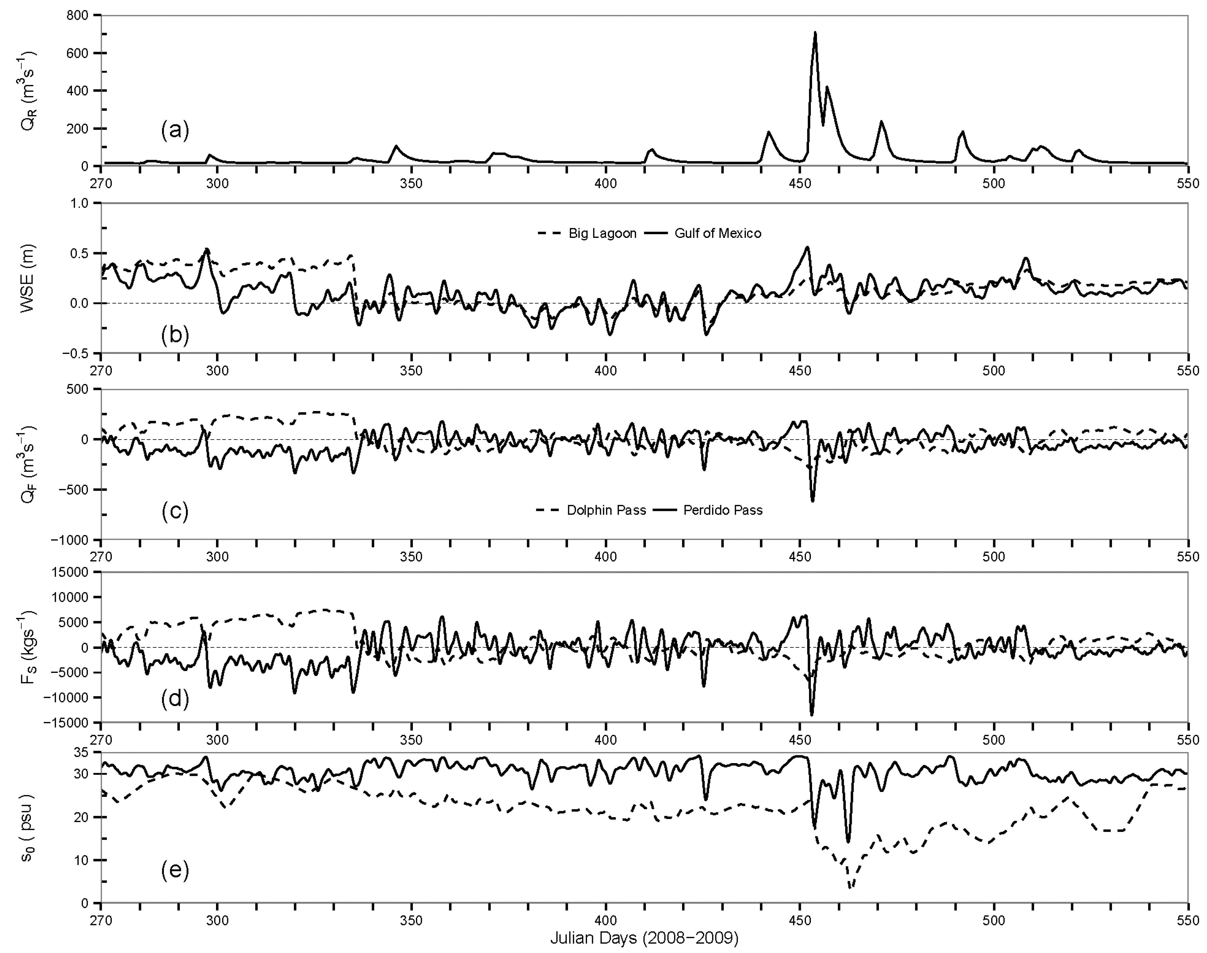
Time series of (a) discharge QR (m3·s−1) from Perdido River and Styx River; (b) water surface elevation (WSE, m) at the Gulf of Mexico (solid line) and Big Lagoon (dashed line); (c) volumetric flow rate QF (m3·s−1); (d) salt transport rate FS (kg·s−1); and (e) cross-sectional average salinity s0 (psu) at Perdido Pass and Dolphin Pass. Positive and negative fluxes in (c) and (d) indicate flow into and out of the Perdido Bay.
Figure 4.
Time series of (a) discharge QR (m3·s−1) from Perdido River and Styx River; (b) water surface elevation (WSE, m) at the Gulf of Mexico (solid line) and Big Lagoon (dashed line); (c) volumetric flow rate QF (m3·s−1); (d) salt transport rate FS (kg·s−1); and (e) cross-sectional average salinity s0 (psu) at Perdido Pass and Dolphin Pass. Positive and negative fluxes in (c) and (d) indicate flow into and out of the Perdido Bay.

Figure 3a shows that salt water was advancing towards the Gulf of Mexico due to the ebb tide (an arrow was used to indicate the flow direction) at the downstream boundary at 15:00 on 25 April 2009 under low inflows from upstream. The Perdido Pass complex includes the area from Perdido Pass (Section A-A) to the Section B-B in Figure 1. The more or less well-mixed condition happened in the Perdido Pass complex with salinity about 34 psu throughout the depth. However, at the intersection of Ross Point and Innerarity Point (~7.5 km upstream from Perdido Pass), the vertical salinity stratification was strong and about 10 psu (11 and 21 psu at the surface and bottom layers, respectively). The salinity stratification decreased rapidly from Ross/Innerarity Point to DuPont Point and US Hwy 98 bridge due to the dilution created from the upstream freshwater inflows. In Figure 3b, at 21:00 on 25 April 2009, reduced salinity towards Perdido Pass indicated that the salinity was greatly reduced from ebb tide to the lowest water surface elevation at the downstream boundary. The Perdido Pass complex during the lowest water surface elevation at downstream had a stronger stratification compared to the stratification under ebb tide (Figure 3a). The strongest stratification occurred in the middle portion of the Perdido Pass complex where the surface salinity ranged from 14–18 psu and the bottom salinity from 28–30 psu (red region in Figure 3b). A snapshot of salinity distribution at 05:00 on 26 April 2009 (Figure 3c) shows that salinity was being introduced into the Perdido Bay by the flood tide from the Gulf of Mexico. During the flood tide, the stratification near Perdido Pass occurred at the lowest elevation (Figure 3b) and was destroyed because the water depth was relatively small and flow momentum from tides was large, and flood tides from downstream eventually pushed high saline water into the system. Because the inflows were small on 25–26 April 2009, salt water passed the US Hwy 98 Bridge (5–8 psu) and reached upper Perdido Bay, but Perdido River mouth still had freshwater under both ebb and flood tides (Figure 3) at Perdido Pass.
During the large inflows from upstream, the salinity at the Perdido Pass complex was relatively small regardless of ebb or flood tides at the Gulf of Mexico [36]. Therefore, complex temporal and spatial stratification patterns in Perdido Bay were the result of interactions between different inflows and tidal variations.
3.3. Eulerian Flux Decomposition in the PBWB System
To explore the salt fluxes into the PBWB system, the Eulerian method of salt flux decomposition was applied to hourly time series data of simulated velocity, water surface elevation, and salinity from calibrated Perdido EFDC model. The flux calculations were performed from 26 September 2008 (Julian Day 270)–3 July 2009 (Julian Day 550). To avoid any effect of initial conditions, the first 20 simulation days were treated as model spin up period. The model forcing includes observed river inflows, ocean tides, and meteorological inputs as boundary conditions. Flow exchanges were calculated at five different cross sections (Figure 1) in the PBWB system. For Eulerian flux method, Equations (1)–(7) were implemented to compute various flux components such as , , , , , , , and . To be consistent about the sign convention, Perdido Bay is treated as the control area or reference area where the flow exchange takes place between Perdido Pass, Dolphin Pass, and Wolf Bay. All flows and fluxes moving from the external (open) boundary, or Wolf Bay into Perdido Bay, have positive values, and all flows and fluxes moving out of Perdido Bay to the external boundary, or Perdido Bay to Wolf Bay, have negative values (Figure 4, Figure 5 and Figure 6 and in Table 3, Table 4 and Table 5).
The 2008–2009 simulation period had a wide range of freshwater river discharges QR (Figure 4a) flowing into Perdido Bay, which ranged from 14.2–760 m3·s−1 with an average inflow of 42.0 m3·s−1. The time series of filtered water surface elevation (WSE) at the Gulf of Mexico during the simulation period plotted in Figure 4b exhibited the variation from −0.32 m up to 0.77 m with an average value of 0.15 m. Filtered WSE at the Big Lagoon (east boundary, Figure 1) varied from −0.19 –0.54 m with an average value of 0.14 m, and was mostly higher than filtered WSE at the Gulf before Julian Day 335 (31 November 2008, Figure 4b). Average values of subtidal volumetric flow rate QF (Figure 4c) calculated from Eulerian flux method (Equation (2)) over the simulation period were −42.5 m3·s−1 and 16 m3·s−1 (Table 3) for Perdido Pass (Section A-A, Figure 1) and Dolphin Pass (Section C-C, Figure 1), respectively. The negative values of discharge QF and salt flux FS indicate seaward flux from Perdido Bay, i.e., southward through Perdido Pass and eastward through Dolphin Pass. Both QF and FS showed large temporal variations. QF through Perdido Pass ranged from −619 m3·s−1–180 m3·s−1 (Table 3). The subtidal salt flux FS through Perdido Pass (Figure 4d and Table 3) ranged from −13,480–6289 kg·s−1 (average of −527 kg·s−1) and −6789–7393 kg·s−1 (average of 648 kg·s−1) through Dolphin Pass. With the range of variations 1–2 orders of magnitude larger than the corresponding means, the mean flux values are not representative of the water and salt exchange through Perdido Pass and Dolphin Pass.
Figure 5.
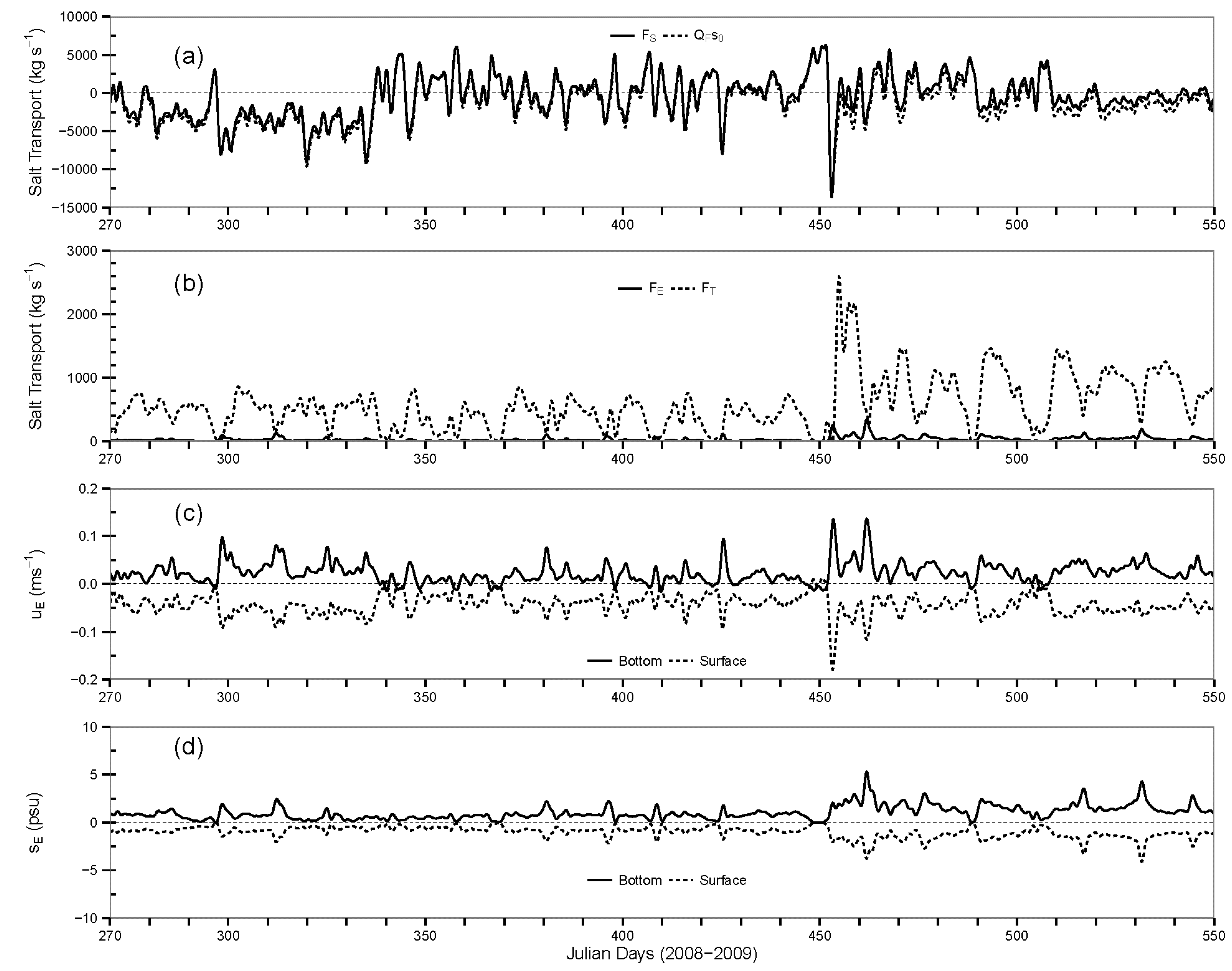
(a) Salt transport rate FS (kg·s−1) and river flow flux component QF so; (b) salt transport components FE and FT through Section A-A (Perdido Pass); (c) subtidal estuarine exchange flow uE (m·s−1); and (d) salinity sE (psu) in the surface and bottom layers at the deepest channel cell of Perdido Pass. Positive (negative) flux in (a) and (b) and positive (negative) velocity in (c) indicate the flow into (out of) Perdido Bay. Note that y-axis scales are different in (a) and (b).
Figure 5.
(a) Salt transport rate FS (kg·s−1) and river flow flux component QF so; (b) salt transport components FE and FT through Section A-A (Perdido Pass); (c) subtidal estuarine exchange flow uE (m·s−1); and (d) salinity sE (psu) in the surface and bottom layers at the deepest channel cell of Perdido Pass. Positive (negative) flux in (a) and (b) and positive (negative) velocity in (c) indicate the flow into (out of) Perdido Bay. Note that y-axis scales are different in (a) and (b).

Figure 6.
Shear dispersion (FE) and tidal oscillatory (FT) salt transport through four cross sections (Figure 1): (a) Perdido Pass complex (Section B-B); (b) Dolphin Pass (Section C-C); (c) Wolf-Perdido canal (Section D-D); and (d) Lower Perdido Bay (Section E-E).
Figure 6.
Shear dispersion (FE) and tidal oscillatory (FT) salt transport through four cross sections (Figure 1): (a) Perdido Pass complex (Section B-B); (b) Dolphin Pass (Section C-C); (c) Wolf-Perdido canal (Section D-D); and (d) Lower Perdido Bay (Section E-E).
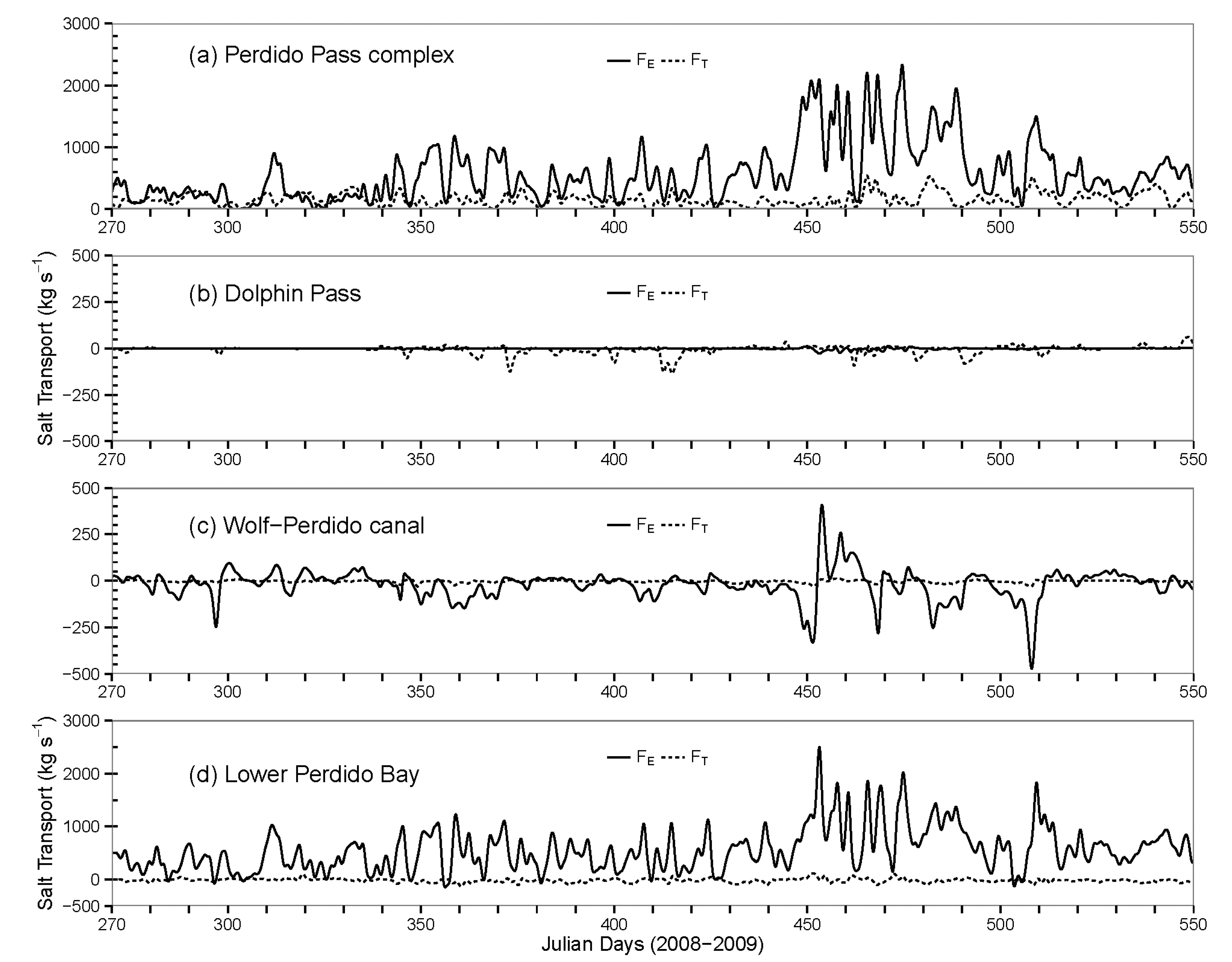
Table 3.
Statistical summary of QF (m3·s−1) and FS (kg·s−1) computed using Eulerian decomposition method through five cross sections (Figure 1): Perdido Pass (Section A-A), the Perdido Pass complex (Section B-B), Dolphin Pass (Section C-C), the Wolf-Perdido canal (Section D-D), and lower Perdido Bay (Section E-E).
| Statistical Parameters | Perdido Pass | Perdido Pass Complex | Dolphin Pass | Wolf-Perdido Canal | Lower Perdido Bay | |||||
|---|---|---|---|---|---|---|---|---|---|---|
| QF | FS | QF | FS | QF | FS | QF | FS | QF | FS | |
| Minimum | −619 | −13,480 | −873 | −14,810 | −286 | −6,789 | −127 | −2,181 | −777 | −11,430 |
| Maximum | 180 | 6,289 | 139 | 4,020 | 272 | 7,393 | 51 | 804 | 94 | 2,198 |
| Mean | −42 | −527 | −34 | 113 | 16 | 648 | −14 | −309 | −50 | −360 |
| Standard Deviation | 98 | 2787 | 95 | 1,862 | 121 | 2,924 | 25 | 472 | 76 | 1,302 |
| 1st Quartile | −101 | −2,114 | −66 | −713 | −75 | −1,474 | −29 | −570 | −71 | −921 |
| Median | −40 | −506 | −15 | 430 | 3 | 44 | −12 | −231 | −36 | −125 |
| 3rd Quartile | 18 | 1,118 | 21 | 1,153 | 89 | 1,852 | 2 | 11 | −10 | 327 |
Table 4.
Correlation coefficients of FE (kg·s−1), FS (kg·s−1), and QF (m3·s−1) through different cross sections (Figure 1).
| Cross SectionsVariables | FE | FS | QF |
|---|---|---|---|
| Combined through Sections A-A and C-C versus through Section B-B | 0.06 | 0.95 | 0.97 |
| Combined through Sections B-B and D-D versus through Section E-E | 0.91 | 0.98 | 0.99 |
Note: The Section A-A is Perdido Pass, B-B is the Perdido Pass complex, C-C is Dolphin Pass, D-D is the Perdido-Wolf canal, and E-E is lower Perdido Bay (Figure 1).
Table 5.
Statistical summary of average percent changes (%) and standard deviations of the differences (numbers in the brackets) of exchange parameters between sensitivity model runs and the calibration run at Perdido Pass, Perdido Pass complex, and Wolf-Perdido canal. The “+50% Q” and “−50% Q” represent the 50% increase and decrease of freshwater inflows from all upstream rivers form the calibration run, respectively.
| Parameter/Location | Perdido Pass | Perdido Pass Complex | Wolf-Perdido Canal | |||
|---|---|---|---|---|---|---|
| +50% Q | −50% Q | +50% Q | −50% Q | +50% Q | −50% Q | |
| FE | −34% | −10% | 41% | −6% | −288% | 3576% |
| (20.2 1) | (18.6) | (180.4) | (121.2) | (42.6) | (87.6) | |
| FT | 20% | −22% | 4% | −19% | 1560% | −1317% |
| (130.7) | (175.8) | (39.5) | (51.6) | (4.0) | (6.1) | |
| FS | −25% | 22% | −1% | 19% | −4% | 10% |
| (223.5) | (301.8) | (218.8) | (282.8) | (61.6) | (95.5) | |
| QF | −44% | 38% | 4% | −8% | −2% | 13% |
| (18.3 2) | (19.0) | (27.0) | (27.2) | (6.9) | (6.5) | |
Notes: 1 in kg s-1 for all numbers in the brackets for FE, FT, and FS; 2 in m3·s−1 for all numbers in the brackets for QF.
Subtidal flow rate QF at Perdido Pass had relatively strong correlation with river discharge QR and filtered WSE at the Gulf (Wgulf) and Big Lagoon boundaries (Wbl). A multi-linear regression equation was developed including above variables, and the regression equation explains 76% variations of QF:
Because QF is negative for seaward flux and QR is positive for flows from upstream, the regression coefficient for QR is negative. The regression equation shows that the seaward flux at Perdido Pass is proportional to upstream river discharge and WSE at Big Lagoon but inversely proportional to WSE at the Gulf. The regression equation approximately indicates that a 100 m3·s−1 of river discharge from upstream is balanced with a 0.12 m WSE increase at the Gulf. The equation shows complex interactions between river discharges from upstream and WSEs directly or indirectly influenced by tides in the Gulf of Mexico. From Equation (8), it is evident that the water surface elevation boundary posed at Big Lagoon and the Gulf of Mexico have a large impact on overall fate and transport of salinity in the estuary.
Figure 4e shows the time series of tidally and sectionally averaged salinity (s0) for Perdido Pass (solid line) and Dolphin Pass (dashed line). From Julian Day 270–330 s0 at Dolphin Pass was in similar order of magnitude compared to the s0 at Perdido Pass. From Julian Days 330–550 s0 at Perdido Pass was much higher. The salinity s0 at Perdido Pass ranged from 14–34 psu with a mean value of 30.4 psu, whereas s0 at Dolphin Pass ranged from 3–30 psu with a mean value of 22 psu. The reason why s0 is higher in Perdido Pass is because Perdido Pass is directly connected to the Gulf of Mexico where a constant salinity of 34 psu was applied, whereas Dolphin Pass is connected to the Gulf through Big Lagoon and Pensacola Bay that have a relatively lower salinity boundary condition applied.
3.4. Exchange through Perdido Pass
The relative contribution of three components (, FE, and FT in Equation (6)) to FS varies as function of water column stratification [23]. For Julian Days 270–450, FS was almost entirely determined by (Figure 5a), which indicates the stratification at Perdido Pass was relatively weak. However, for Julian Days 450–550, the shear dispersive salt transport FE and the tidal oscillatory salt transport FT (Figure 5b, different y-axis scale from Figure 5a) were significant and were equally important as , which indicates a relatively strong stratification at Perdido Pass. The FT at Perdido Pass (Section A-A in Figure 1) was a dominant or important component of FS in addition to , because velocity and salinity components and were dominant or relatively large, as it is close to the Gulf of Mexico and within a tidal excursion. Dronkers and van de Kreeke [37] suggested that the larger magnitude of oscillatory flux, also called “nonlocal” salt transport, whose magnitude is a function of a variation of topography within a tidal excursion, plays a significant role rather than processes representative of the overall salt transport in an estuary. Many theoretical and numerical studies of salt transport mechanisms have considered estuaries of a uniform cross section [10,38,39]. The Section A-A at Perdido Pass where the salt flux was studied doesn’t have uniform-depth cross section and is characterized by narrow width with deep channel and shallow overbank areas connecting Perdido Bay and the Gulf of Mexico. The sudden change in the area of flow and bathymetry between the Gulf of Mexico and Perdido Pass and between Perdido Pass and Perdido Bay can result in large horizontal dispersion (see more information in the Section 3.7) and the domination of FT component at Perdido Pass. For Julian Days 450–560, FT increased largely compared to FT from 250–450 (Figure 5b); this is due to the interaction of large inflows from upstream and variations of downstream tides. FE at Perdido Pass was up to 346 kg·s−1 (Figure 5b) with an average value of 31 kg·s−1 , but FT was up to 2596 kg·s−1 with an average value of 582 kg·s−1. FT at Perdido Pass was on the average 19 times larger than FE, and they are weakly correlated (correlation coefficient R = 0.34).
In Figure 5c,d exchange flow velocity and salinity (uE and sE) are displayed for surface and bottom layers at the deepest cell in the Perdido Pass cross section. These tidally averaged and sectionally varying velocities were dominantly positive values in the bottom layer but negative values in the surface layer. It means that the exchange flow velocity was dominantly seaward at the surface and landward at the bottom. The exchange flow velocity at the surface was strongly correlated to the velocity at the bottom and the correlation coefficient between them was −0.88. The data analysis shows that the exchange flow salinity sE at the bottom layer was always positive because the bottom salinity was greater than the tidally and sectionally averaged salinity , but sE at the surface layer was always negative because the surface salinity was less than because the interaction with freshwater from upstream rivers. The magnitude of exchange flow salinity at the bottom layer was similar to the salinity in the surface layer with a correlation coefficient of −0.96 (Figure 5d). The estuarine salinity at the deep channel of Perdido Pass varied with moderate variation in stratification. Maximum stratification at Perdido Pass occurred on Julian Days 450–560 with the bottom-surface salinity difference as large as 9 psu, whereas weak stratifications existed from Julian Days 270–450, with ranging from 0–5.2 psu. Variation in stratification was largely determined by complex interactions of river discharges and tidal WSEs. The increase in river inflows from Julian Days 450–560 increased the stratification in Perdido Pass. The exchange flow, defined as the difference between the surface and bottom , had an average value of 0.06 m·s−1 and a maximum value up to 0.19 m·s−1.
In summary, from the Perdido Pass connection, the average salt flux going out of Perdido Bay is −527 kg·s−1 and the average salt flux coming into the estuary from the Gulf of Mexico is 648 kg·s−1. The average tidally and cross-sectionally averaged salinity at the Perdido Pass connection was 30.4 psu. The above provides the information to the first question posed in the end of the introduction.
3.5. Exchange through the Perdido Pass Complex and Dolphin Pass
Eulerian flow decomposition method was also applied to determine the flow exchange components through Sections B-B (Perdido Pass complex), C-C (Dolphin Pass), D-D (the Wolf-Perdido canal), and E-E (the lower Perdido Bay) in Figure 1, that would allow us to investigate the underlying factors that govern salt flux exchange through these cross sections. The distributions of salt flux components FE and FT are different in the Perdido Pass complex (Figure 6a) compared to the components in Perdido Pass (Figure 5b). The dominance of tidal oscillatory flux FT was greatly reduced and exchange flux FE became dominant in the Perdido Pass complex. The salinity and momentum differences between the incoming water flux from the Gulf and outgoing water flux from upstream controlled the amount of flow exchange through Section B-B. The water and salt exchange at the Perdido Pass complex was also affected by western/eastern fluxes from Dolphin Pass (Figure 1) in addition to seaward/landward fluxes from Perdido Pass.
Subtidal averaged QF through Section B-B varied from 139 m3·s−1 (incoming flux) to −873 m3·s−1 (outgoing flux, Table 3). The average value of QF from Julian Days 270–550 through Section B-B was −34 m3·s−1, which was slightly smaller than average QF at Perdido Pass (Figure 5c). The salt flux FS through Section B-B ranged from −14,810–4020 kg·s−1 (average of 113 kg·s−1). In comparison to FE (ranged from −27.9–14.0 kg·s−1 with an average value of −0.5 kg·s−1) through Section C-C (Dolphin Pass, Figure 6b), FT was dominant (ranged from −134.7–61.1 kg·s−1 with an average value of −5.6) and flow exchange occurred in the east-west direction. FT was dominant because the salinities of incoming and outgoing water through Dolphin Pass were not much different, and were directly influenced by the Big Lagoon boundary which is far away from the Gulf of Mexico. Subtidal QF through Section C-C (Dolphin Pass) varied from −286 m3·s−1 (western flux) to 272 m3·s−1 (eastern flux) with a small average value of 16 m3·s−1 (Table 3) in 2008–2009. It means that there were relatively large flows back and forth in the east-west directions through Dolphin Pass but the net flow was not significant.
3.6. Exchange through the Wolf-Perdido Canal and Lower Perdido Bay
The flow exchanges at the Wolf-Perdido canal (Section D-D in Figure 1), which connects Perdido Bay and Wolf Bay, and in lower Perdido Bay (Section E-E) take place in the east-west direction. At the Wolf-Perdido canal, FE was dominant (ranged from −472.2–407.7 kg·s−1 with an average value of −20.5 kg·s−1) and the negative value of FE indicated that the flow was moving from Perdido Bay to Wolf Bay (Figure 6c) due to inflows from upstream rivers into Perdido Bay. QF at the Wolf-Perdido canal varied from −127.2 m3·s−1 (towards Wolf Bay) to 51.1 m3·s−1 (towards Perdido Bay). It means that a small portion of river discharges QR from Perdido River and Styx River could flow through Section D-D into Wolf Bay. On average, there were more days for flows from Perdido Bay to Wolf Bay through Section D-D because average QF at D-D was −14 m3·s−1. QF at the Wolf-Perdido canal was typically smaller than QF at Perdido Pass and Dolphin Pass. The salt-water intrusion from Perdido Bay towards Wolf Bay mostly occurred when there were large inflows from upstream and large incoming flows via the Dolphin Pass and Perdido Pass boundaries. The amount of flow entering Wolf Bay from Perdido Bay was of small magnitude, which might be one of the reasons that Wolf Bay is pristine and less polluted than Perdido Bay. At lower Perdido Bay, FE was dominant with mean value of 556.3 kg·s−1 and mean FT was −15.7 kg·s−1. QF at lower Perdido Bay ranged from −776.5–93.5 m3·s−1 with an average value of −49.5 m3·s−1 (75% of QF is less than −10.0 m3·s−1 or seaward outflows). The salt flux FS at lower Perdido Bay ranged from −11,430 kg s−1 –2198 kg·s−1 with an average value of −360 kg·s−1 (Table 3).
A data analysis was performed to examine possible correlations of salt and flow fluxes FE, FS, and QF through different cross sections. Figure 1 shows that the sum or combined salt and flow fluxes through the Perdido Pass complex (Section B-B) and the Wolf-Perdido canal (Section D-D) would possibly correlate with corresponding fluxes through lower Perdido Bay (Section E-E). It is also possible that the sum or combined salt and flow fluxes through Perdido Pass (Section A-A) and Dolphin Pass (Section C-C) would correlate with corresponding fluxes through the Perdido Pass complex (Figure 1). Derived correlation coefficients of FE, FS, and QF between above-mentioned cross sections are summarized in Table 4. The interaction among exchange salt fluxes FE through the Perdido complex, Dolphin Pass, and Perdido Pass was complex. Therefore, the correlation coefficient between the sum of FE through Perdido Pass and Dolphin Pass and FE through the Perdido Pass complex was very small (only 0.06) because tidal oscillatory flux FT was dominant at Perdido Pass. Other correlation coefficients ranged from 0.91–0.99 (Table 4) indicating that strong correlations of FE, FS, and QF indeed exist between these cross sections.
Thus, we explored the salt exchange between Wolf Bay and Perdido Bay by analyzing the salt flux at the Wolf-Perdido canal. On average, the flow moved from Perdido Bay towards Wolf Bay with a magnitude of 14 m3·s−1 and the average salt flux towards Wolf Bay was 309 kg·s−1. However, these numbers might change when there is a large river inflow from upstream of Perdido Bay and when there is a large flow from Big Lagoon and the Gulf of Mexico. Understanding the overall flow pattern in such navigational systems would allow the water quality manager to make remedial measures if Perdido Bay is polluted.
3.7. Horizontal Dispersion
Dispersion is an important mixing characteristic in an estuary and causes pollutants to spread. Dispersion is the result of velocity differences in space. Following Lerczak et al. [22], the one dimensional along-estuary (x coordinate in equations below) salt conservation equation can be written in the following form:
Integrating the above equation and simplifying it, we get,
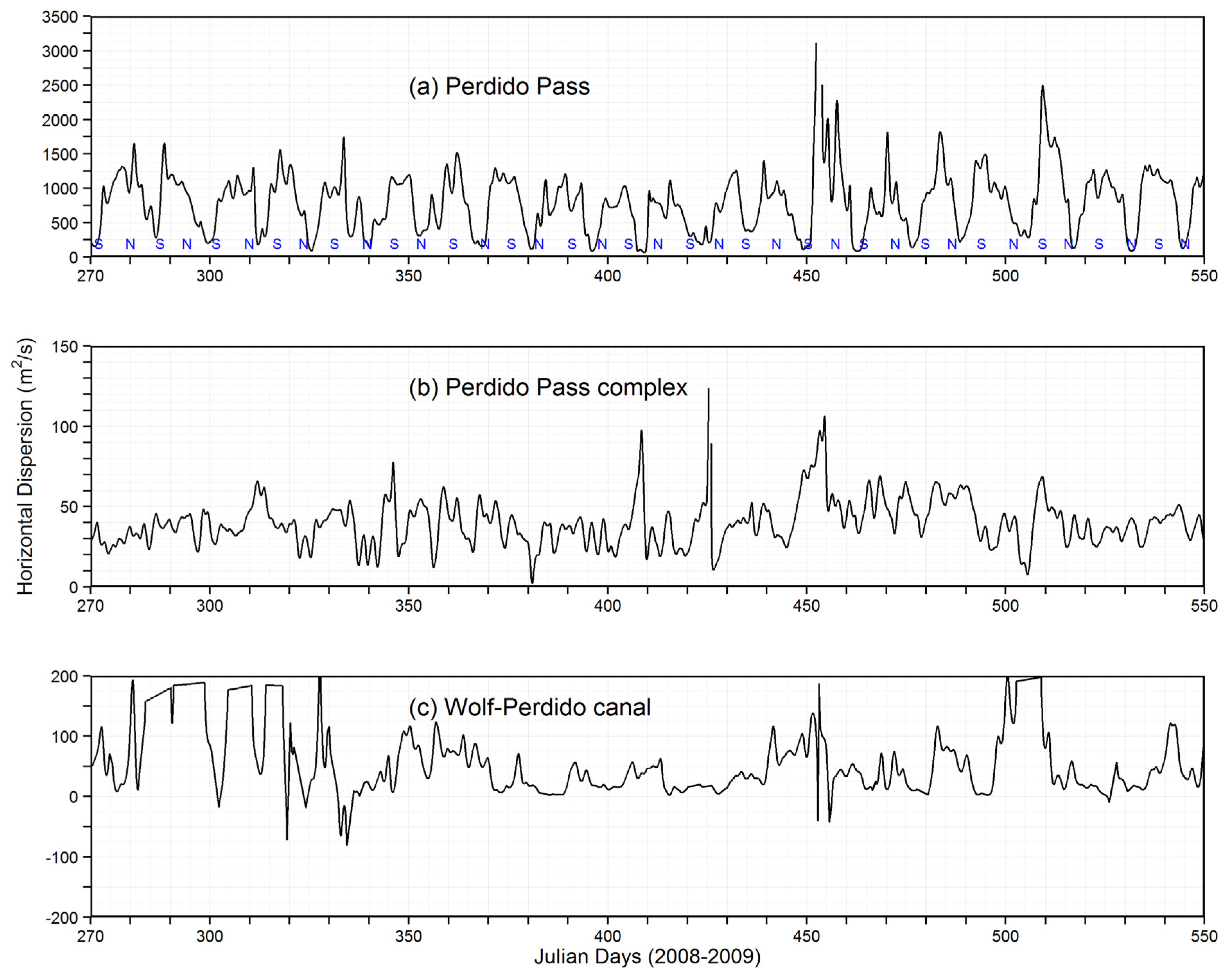
Horizontal dispersion coefficient Kx was calculated using Equation (10) at three locations: Perdido Pass, Perdido Pass complex, and Wolf-Perdido canal. Three time series of Kx were plotted in Figure 7 with different y axis scales for three locations. The magnitude of horizontal dispersion along Perdido Pass was significantly higher compared to the horizontal dispersion at Perdido Pass complex and Wolf-Perdido canal. During the calibration period, the mean horizontal dispersion at Perdido Pass was 810.2 m2/s whereas the mean horizontal dispersion at Perdido Pass complex and Wolf-Perdido canal were 40.2 m2/s and 48.12 m2/s, respectively. When the rate of change of the cross sectionally and time averaged salinity So with respect to the distance does not exactly correspond to the sign change for FE + FT (Equation (10)), horizontal dispersion coefficients at Wolf-Perdido canal during certain time periods were negative (Figure 5c) because of the complex exchange characteristics at the Wolf-Perdido canal (Figure 6c).
The fact that tidal oscillatory flux FT at Perdido Pass (Figure 5b) is dominant and significantly larger explains the higher magnitude of horizontal dispersion at Perdido Pass compared to other cross sections. The magnitude of horizontal dispersion at Perdido Pass was approximately 10 times larger than horizontal dispersion at Perdido Pass complex, which is because of its narrow width and long channel with the direct connection to the Gulf compared to the relatively wide cross section at Perdido Pass complex. The magnitude of Kx at Perdido Pass shows positive correlation with spring (S on Figure 7) and neap (N) tides.
3.8. Sensitivity Experiments
Two sensitivity numerical experiments were performed to evaluate the impact of freshwater into the system. The sensitivity experiments include two model runs with 50% increase and 50% decrease of freshwater inflows (Q) from all rivers into Wolf Bay and Perdido Bay. The water surface elevation boundaries (tidal influences) at the Gulf, Dolphin Pass and GIWW remained unchanged for both the sensitivity runs. The simulation results from the sensitivity model runs were then compared with results from the calibration run. The exchange parameters FE and FT for three cross sections: Perdido Pass, Perdido Pass complex, and Wolf-Perdido canal are plotted in Figure 8. The summary of statistics showing the average percent changes (%) and standard deviations of the differences (numbers in the brackets) of exchange parameters from the calibration run for FE, FT, FS and QF are given in Table 5. The exchange parameters at different locations have different orders of magnitude and different directions. Therefore, to provide more insights in the interactions due to increase and decrease of freshwater inflows, both percent changes and standard deviations in kg·s−1 or m3·s−1 of the differences are presented in Table 5. When the magnitudes of parameters such as QF, FE, FT and FS in the calibration run are small (near zero) in certain periods, the percent changes from the calibration run would be larger numbers, which would eventually impact the average percent change. It should be noted that since the interactions among various forcing factors are complex in an estuary, both graphical and tabular results only provide partial information.
Figure 7.
Horizontal dispersion (Kx) at three cross sections (Figure 1): (a) Perdido Pass; (b) Perdido Pass complex; and (c) Wolf-Perdido canal. The “S” and “N” in the top panel stand for spring and neap tides.
Figure 7.
Horizontal dispersion (Kx) at three cross sections (Figure 1): (a) Perdido Pass; (b) Perdido Pass complex; and (c) Wolf-Perdido canal. The “S” and “N” in the top panel stand for spring and neap tides.
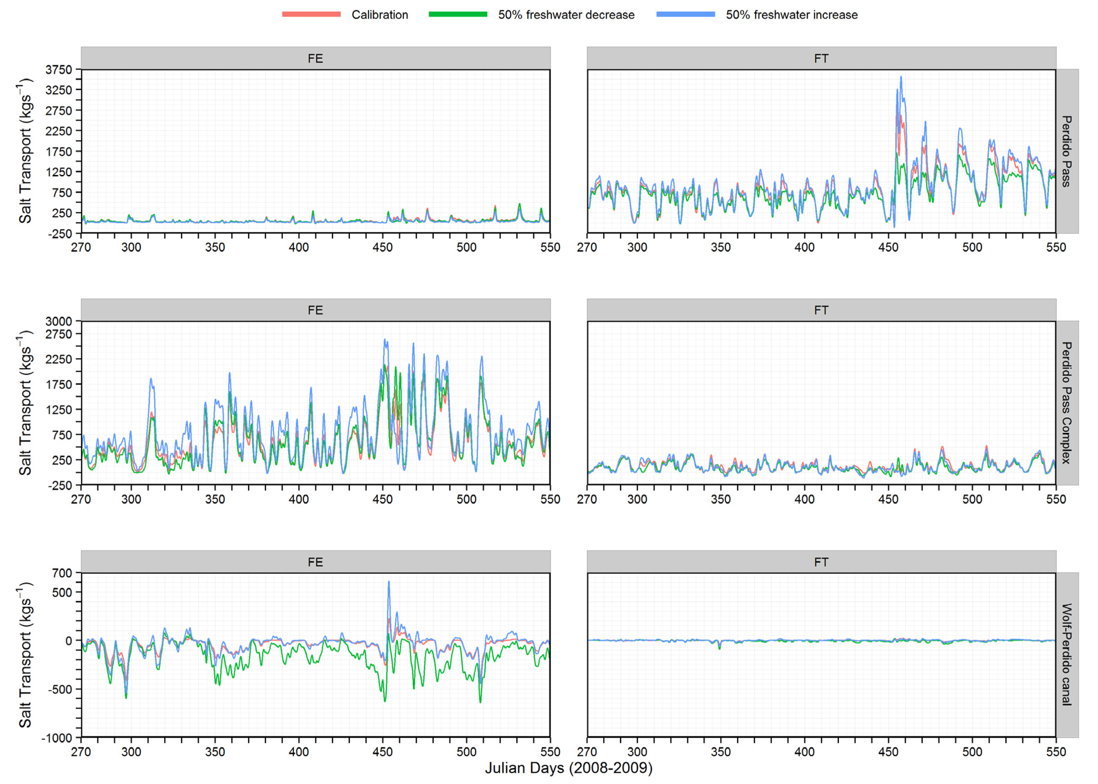
At Perdido Pass, total salt flux FS would decrease on average by 25% for 50% Q increase, while it would increase by 22% for 50% Q decrease. This is because these results are more dominated by the tidal boundary at the Gulf, which is the same for sensitivity runs and the calibration run. The oscillatory flux FT depends on characteristics of tidal excursion and local bathymetry. FT exchange component, which is dominant in Perdido Pass, would increase on average by 20% with 50% Q increase, while FT would decrease by 22% with 50% Q decrease. On average (Table 5), the shear dispersive transport component FE at Perdido Pass would have smaller magnitude for both 50% increase and decrease of freshwater inflows.
At Perdido Pass complex, the salt flux component FE with 50% Q increase would have consistent increase compared to the calibration run. This is because higher upstream inflow from Perdido Bay would cause the flow on upper layers to rapidly propagate towards the Gulf and increase overall stratification and dispersion. FE with 50% Q decrease would have on average a small drop compared to the calibration run, except during Julian days 450–460, where there was a large inflow coming into the system from the rivers upstream of Perdido Bay.
Figure 8.
Time series of shear dispersive transport (FE) and oscillatory tidal transport (FE) at Perdido Pass, Perdido Pass complex, and Wolf-Perdido canal for the calibration run, 50% freshwater increase and 50% freshwater decrease sensitivity runs.
Figure 8.
Time series of shear dispersive transport (FE) and oscillatory tidal transport (FE) at Perdido Pass, Perdido Pass complex, and Wolf-Perdido canal for the calibration run, 50% freshwater increase and 50% freshwater decrease sensitivity runs.
4. Summary and Conclusions
A previously calibrated three-dimensional hydrodynamic EFDC model was used to simulate flow and salinity distributions in the Perdido Bay and Wolf Bay system under unsteady flows from rivers, tides from three open boundaries, and atmospheric forcing in 2008–2009. The calibrated EFDC model provided simulated hourly velocities and salinity at different layers (depths) for all grids in five cross sections. Eulerian flux method was applied to determine the water and salt fluxes through these cross sections using hourly model outputs. The summaries of key findings from the study are as follows:
- The salinity at Perdido Bay varied largely with upstream inflows (low and high inflows) and tides at open boundaries (ebb and flood tides). Inflow of highly saline water at the bottom layers and outflow of relative low salinity water at the surface layers resulted from the interaction of flood tide at the Gulf of Mexico and inflows from upstream. Salinity was always small from the US Hwy 98 Bridge towards Perdido River. During low inflows from upstream and flood tides from the Gulf of Mexico, maximum salinity up to 32 psu reached Ross/Innerarity Point (lower Perdido Bay).
- Eulerian analysis concluded that tidal oscillatory fluxes (FT) at Perdido Pass (Section A-A) and Dolphin Pass (Section C-C) were dominant compared to exchange flow component FE, whereas at Sections B-B (Perdido Pass complex), D-D (Wolf-Perdido canal), and E-E (lower Perdido Bay) the exchange flows FE were dominant.
- During the simulation period, it was found that a small amount of flow exchange occurred between Wolf Bay and Perdido Bay. During the high inflows from rivers in Perdido Bay and higher tides from the Gulf and Big Lagoon, the water from Perdido Bay moved towards Wolf Bay, however, during normal flows and gentle tides the water from Wolf Bay moved towards Perdido Bay. It means the influences from Perdido Bay and the Gulf of Mexico was relatively small in Wolf Bay under normal inflows.
- Horizontal dispersion coefficient was computed at three locations for the calibration run and it was found that the magnitude of horizontal dispersion at Perdido Pass (a relatively narrow channel which directly connects to the Gulf) was approximately 10 times larger than horizontal dispersion coefficient at Perdido Pass complex (wide cross section).
- Sensitivity runs with 50% increase and 50% decrease in freshwater inflow relative to the calibration run were performed. At Perdido Pass, total salt flux FS would decrease on average by 25% for 50% Q increase while it would increase by 22% for 50% Q decrease, because tidal boundary at the Gulf is fixed for the calibration and sensitivity runs.
Acknowledgments
This study was partially funded through the project “Impacts of human activities and climate change on water resources and ecosystem health in the Wolf Bay Basin: A Coastal Diagnostic and Forecast System (CDFS) for integrated assessment” by Auburn University Water Resources Center. The authors would like to thank the reviewers for providing valuable comments that helped us to improve the manuscript.
Author Contributions
Authors collaborated together for the completion of this work. Janesh Devkota designed the study, developed and calibrated the Perdido EFDC model, ran the model for all cases, performed data analyses of model results and wrote the first draft of the manuscript. Xing Fang provided valuable instructions on study design, supervised the data analyses, and reviewed and revised the manuscript. Both authors contributed significantly in writing the manuscript.
Conflicts of Interest
The authors declare no conflict of interest.
References
- Neilson, B.J.; Cronin, L.E. Estuaries and Nutrients; Humana Press: Clifton, NJ, USA, 1981. [Google Scholar]
- Kennish, M.J. Ecology of Estuaries, Volume i: Physical and Chemical Aspects; CRC Press, Inc.: Boca Raton, FL, USA, 1986; p. 254. [Google Scholar]
- Bilgili, A.; Proehl, J.A.; Lynch, D.R.; Smith, K.W.; Swift, M.R. Estuary/ocean exchange and tidal mixing in a gulf of maine estuary: A lagrangian modeling study. Estuar. Coast. Shelf Sci. 2005, 65, 607–624. [Google Scholar] [CrossRef]
- Ketchum, B.H. The exchanges of fresh and salt waters in tidal estuaries. J. Marine Res. 1951, 10, 18–38. [Google Scholar]
- MacCready, P. Calculating estuarine exchange flow using isohaline coordinates. J. Phys. Oceanogr. 2011, 41, 1116–1124. [Google Scholar] [CrossRef]
- Lewis, R.E.; Lewis, J.O. The principal factors contributing to the flux of salt in a narrow, partially stratified estuary. Estuar. Coast. Shelf Sci. 1983, 16, 599–626. [Google Scholar] [CrossRef]
- Jay, D.A.; Musiak, J.D. Internal tidal asymmetry in channel flows: Origins and consequences. Coast. Estuar. Stud. 1996, 211–249. [Google Scholar] [CrossRef]
- Fischer, H.B. Mixing and dispersion in estuaries. Annu. Rev. Fluid Mech. 1976, 8, 107–133. [Google Scholar] [CrossRef]
- Hansen, D.V.; Rattray, M., Jr. New dimensions in estuary classification. Limnol. Oceanogr. 1966, 319–326. [Google Scholar] [CrossRef]
- Smith, R. Buoyancy effects upon longitudinal dispersion in wide well-mixed estuaries. Philos. Trans. R. Soc. Lond. Ser. A Math. Phys. Sci. 1980, 296, 467–496. [Google Scholar] [CrossRef]
- Uncles, R.J.; Stephens, J.A. Salt intrusion in the tweed estuary. Estuar. Coast. Shelf Sci. 1996, 43, 271–293. [Google Scholar] [CrossRef]
- Fischer, H.B.; List, E.J.; Koh, R.C.Y.; Imberger, J.; Brooks, N.H. Mixing in Inland and Coastal Waters; Academic Press: San Diego, CA, USA, 1979. [Google Scholar]
- MacDonald, D.G. Estimating an estuarine mixing and exchange ratio from boundary data with application to mt. Hope bay (massachusetts/rhode island). Estuar. Coast. Shelf Sci. 2006, 70, 326–332. [Google Scholar] [CrossRef]
- Gilcoto, M.; Pardo, P.C.; Alvarez-Salgado, X.A.; Perez, F.F. Exchange fluxes between the ria de vigo and the shelf: A bidirectional flow forced by remote wind. J. Geophys. Res.-Oceans 2007, 112. [Google Scholar] [CrossRef]
- Traynum, S.; Styles, R. Exchange flow between two estuaries connected by a shallow tidal channel. J. Coast. Res. 2008, 24, 1260–1268. [Google Scholar] [CrossRef]
- Engqvist, A.; Stenstrom, P. Flow regimes and long-term water exchange of the himmerfjarden estuary. Estuar. Coast. Shelf Sci. 2009, 83, 159–174. [Google Scholar] [CrossRef]
- Valle-Levinson, A.; Gutierrez de Velasco, G.; Trasviña, A.; Souza, A.; Durazo, R.; Mehta, A. Residual exchange flows in subtropical estuaries. Estuar. Coasts 2009, 32, 54–67. [Google Scholar] [CrossRef]
- Chen, S.N.; Geyer, W.R.; Ralston, D.K.; Lerczak, J.A. Estuarine exchange flow quantified with isohaline coordinates: Contrasting long and short estuaries. J. Phys. Oceanogr. 2012, 42, 748–763. [Google Scholar] [CrossRef]
- Devkota, J.; Fang, X.; Fang, V.Z. Response characteristics of perdido and wolf bay system to inflows and sea level rise. Br. J. Environ. Clim. Chang. 2013, 3, 229–256. [Google Scholar] [CrossRef]
- Xia, M.; Craig, P.M.; Wallen, C.M.; Stoddard, A.; Mandrup-Poulsen, J.; Peng, M.; Schaeffer, B.; Liu, Z. Numerical simulation of salinity and dissolved oxygen at perdido bay and adjacent coastal ocean. J. Coast. Res. 2011, 27, 73–86. [Google Scholar] [CrossRef]
- Xia, M.; Xie, L.; Pietrafesa, L.J.; Whitney, M.M. The ideal response of a gulf of mexico estuary plume to wind forcing: Its connection with salt flux and a lagrangian view. J. Geophys. Res. 2011, 116, C08035. [Google Scholar]
- Lerczak, J.A.; Geyer, W.R.; Chant, R.J. Mechanisms driving the time-dependent salt flux in a partially stratified estuary. J. Phys. Oceanogr. 2006, 36, 2296–2311. [Google Scholar] [CrossRef]
- Kim, C.-K.; Park, K. A modeling study of water and salt exchange for a micro-tidal, stratified northern gulf of mexico estuary. J. Marine Syst. 2012, 96–97, 103–115. [Google Scholar] [CrossRef]
- Livingston, R.J. Trophic Organization in Coastal Systems; CRC Press: Boca Raton, FL, USA, 2003. [Google Scholar]
- Duchon, C.E. Lanczos filtering in one and two dimensions. J. Appl. Meteorol. 1979, 18, 1016–1022. [Google Scholar] [CrossRef]
- Wang, R.; Kalin, L. Modelling effects of land use/cover changes under limited data. Ecohydrology 2011, 4, 265–276. [Google Scholar] [CrossRef]
- Beasley, L.R. Interaction of Groundwater,Surface Water and Seawater in Wolf Bay, Weeks Bay, and Dauphin Island Coastal Watersheds, Alabama; Auburn University: Auburn, AL, USA, 2010. [Google Scholar]
- Hamrick, J.M. A Three-Dimensional Environmental Fluid Dynamics Computer Code: Theoretical and Computational Aspects; Special Report 317; Virginia Institute of Marine Science, College of William and Mary: Gloucester Point, VA, USA, 1992. [Google Scholar]
- Hamrick, J.M.; Mills, W.B. Analysis of water temperatures in conowingo pond as influenced by the peach bottom atomic power plant thermal discharge. Environ. Sci. Policy 2000, 3, 197–209. [Google Scholar] [CrossRef]
- Park, K.; Jung, H.-S.; Kim, H.-S.; Ahn, S.-M. Three-dimensional hydrodynamic-eutrophication model (hem-3d): Application to kwang-yang bay, korea. Marine Environ. Res. 2005, 60, 171–193. [Google Scholar] [CrossRef]
- Mellor, G.L.; Yamada, T. Development of a turbulence closure model for geophysical fluid problems. Rev. Geophys. Space Phys. 1982, 20, 851–875. [Google Scholar] [CrossRef]
- Galperin, B.; Kantha, L.H.; Hassid, S.; Rosati, A. A quasi-equilibrium turbulent energy model for geophysical flows. J. Atmos. Sci. 1988, 45, 55–62. [Google Scholar] [CrossRef]
- Gong, W.; Shen, J.; Hong, B. The influence of wind on the water age in the tidal rappahannock river. Marine Environ. Res. 2009, 68, 203–216. [Google Scholar] [CrossRef]
- Godin, G. The Analysis of Tides; University of Toronto Press: Toronto, ON, Canada, 1972; p. 264. [Google Scholar]
- Processing and Publication of Discharge and State Data Collected in Tidally-Influenced Areas. Available online: http://water.usgs.gov/admin/memo/SW/sw10.08-final_tidal_policy_memo.pdf (accessed on 1 March 2014).
- Sterling, M.; Beaman, F.; Morvan, H.; Wright, N. Bed-shear stress characteristics of a simple, prismatic, rectangular channel. J. Eng. Mech. 2008, 134, 1085–1094. [Google Scholar] [CrossRef]
- Dronkers, J.; van de Kreeke, J. Experimental determination of salt intrusion mechanisms in the volkerak estuary. Neth. J. Sea Res. 1986, 20, 1–19. [Google Scholar] [CrossRef]
- Fischer, H.B. Mass transport mechanisms in partially stratified estuaries. J. Fluid Mech. 1972, 53, 671–687. [Google Scholar] [CrossRef]
- Scott, C.F. A numerical study of the interaction of tidal oscillations and non-linearities in an estuary. Estuar. Coast. Shelf Sci. 1994, 39, 477–496. [Google Scholar] [CrossRef]
© 2015 by the authors; licensee MDPI, Basel, Switzerland. This article is an open access article distributed under the terms and conditions of the Creative Commons Attribution license (http://creativecommons.org/licenses/by/4.0/).
Share and Cite
MDPI and ACS Style
Devkota, J.; Fang, X. Quantification of Water and Salt Exchanges in a Tidal Estuary. Water 2015, 7, 1769-1791. https://doi.org/10.3390/w7051769
AMA Style
Devkota J, Fang X. Quantification of Water and Salt Exchanges in a Tidal Estuary. Water. 2015; 7(5):1769-1791. https://doi.org/10.3390/w7051769
Chicago/Turabian StyleDevkota, Janesh, and Xing Fang. 2015. "Quantification of Water and Salt Exchanges in a Tidal Estuary" Water 7, no. 5: 1769-1791. https://doi.org/10.3390/w7051769