
Assessment of the Impacts of Climate Change on the Water Quality of a Small Deep Reservoir in a Humid-Subtropical Climatic Region

 ,
,
Abstract
:1. Introduction
2. Materials and Methods
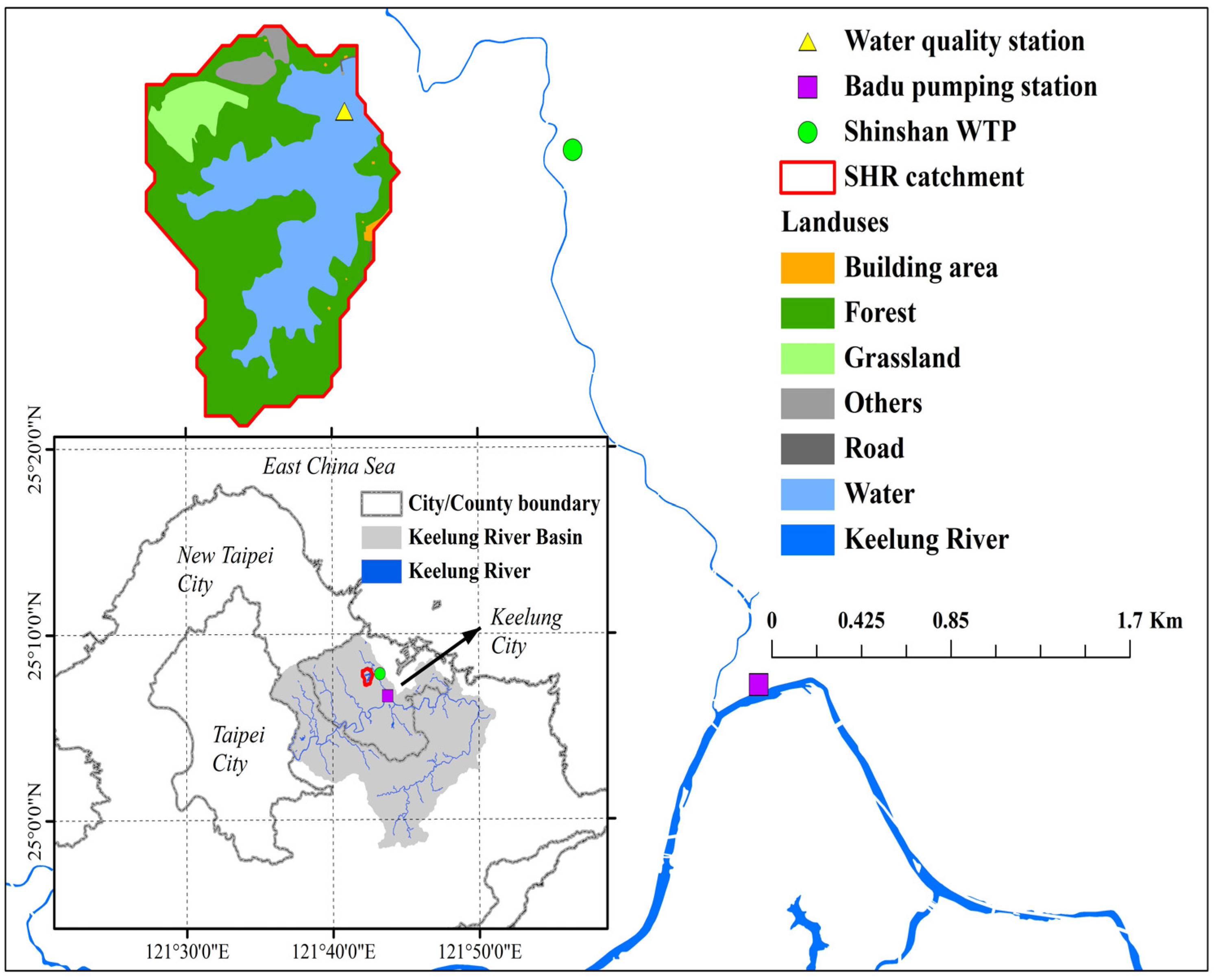
2.1. Study Area
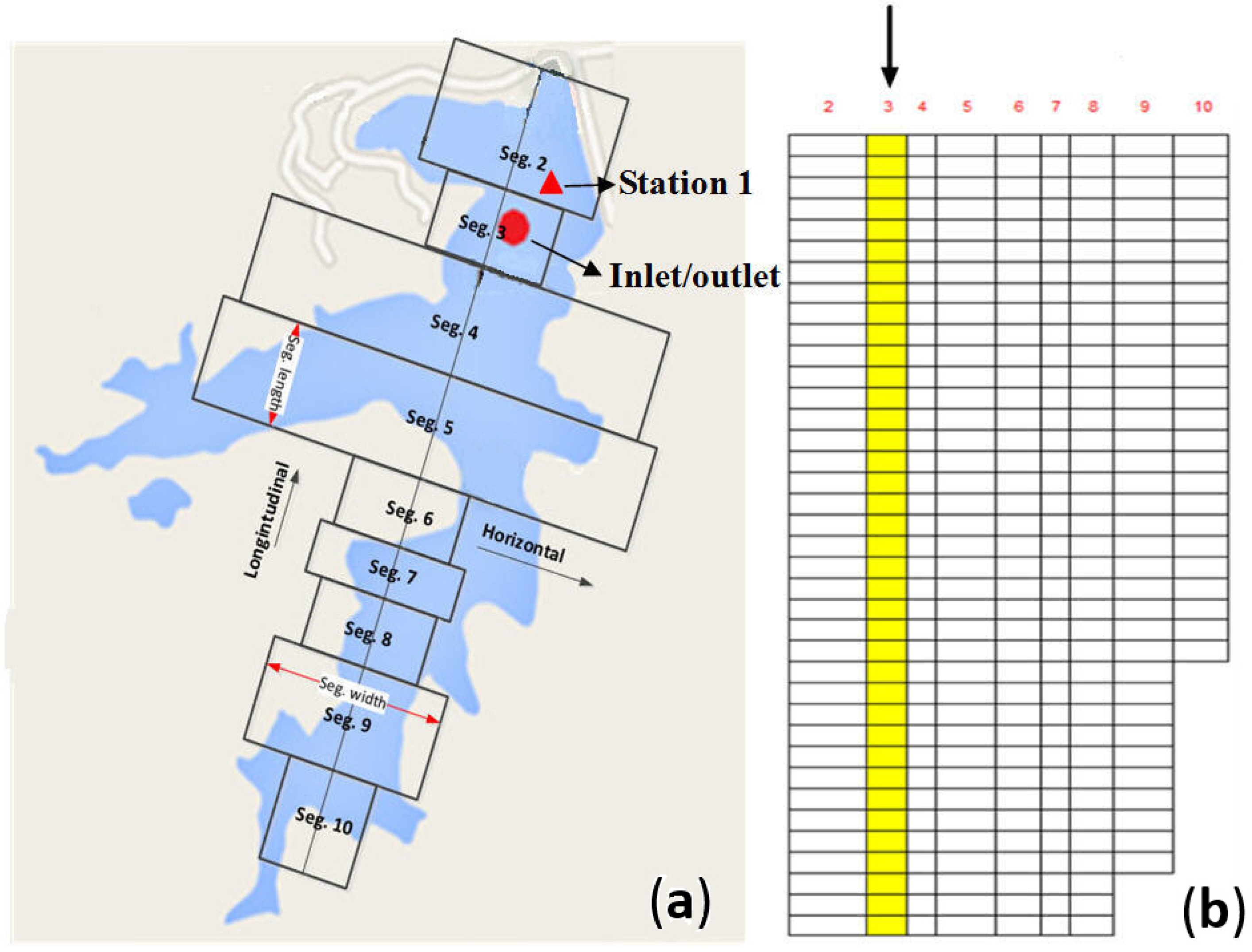
2.2. CE-QUAL-W2 Model

2.3. Climate Change Data

| Climate Variable | Selected Climate Model | |||
|---|---|---|---|---|
| 2020–2039 | 2080–2099 | |||
| A1B | A2 | A1B | A2 | |
| Temperature LL 10% | MRI-CGCM 2.3.2 | CGCM 3.1 (T47) | AOM 4x3 | ECHAM 4.6 |
| Temperature LL 25% | AOM 4 × 3 | ECHAM 5/MPI-OM | AOM 4x3 | PCM 1.0 |
| Temperature UL 75% | CCSM 3.0 | CCSM 3.0 | MIROC 3.2 | MIROC 3.2 |
| Temperature UL 90% | MIROC 3.2 | CCSM 3.0 | MIROC 3.2 | MIROC 3.2 |
| Rainfall LL 10% | BCM 2.0 | BCM 2.0 | BCM 2.0 | BCM 2.0 |
| Rainfall LL 25% | BCM 2.0 | BCM 2.0 | GISS Model ER | GISS Model ER |
| Rainfall UL 75% | BCM 2.0 | BCM 2.0 | CM 2.0 | BCM 2.0 |
| Rainfall UL 90% | CSIRO Mark 3.0 | CGCM 3.1 (T47) | MRI-CGCM 2.3.2 | BCM 2.0 |
2.4. Data Collection
2.5. Model Calibration and Validation Procedure
| Model Parameter | Parameter Range | HSR |
|---|---|---|
| Light extinction for pure water (m−1) | 0.25 or 0.45 | 0.45 |
| Light extinction due to suspended solids (m−1) | 0–0.1 | 0.01 |
| Suspended solids settling rate (m·d−1) | - | 1.0 |
| Sediment release rate of phosphorus (fraction of SOD) | 0.001–0.015 | 0.023 |
| Sediment release rate of ammonium (fraction of SOD) | 0.001–0.03 | 0.03 |
| Ammonia decay rate (d−1) | 0.001–0.95 | 0.5 |
| Nitrate decay rate (d−1) | 0.03–0.15 | 0.03 |
| Maximum algal growth rate (d−1) | 0.17–11.0 | 1.3 |
| Algal settling rate (m·d−1) | 0.0–30.2 | 0.05 |
| Light saturation intensity at max. photosynthetic rate (W·m−2) | 10–170 | 55 |
| Algal half-saturation for phosphorus limited growth (g·m−3) | 0.001–1.52 | 0.0038 |
| Algal half-saturation for nitrogen limited growth (g·m−3) | 0.001–4.34 | 0.022 |
2.6. Risk Analysis

3. Results and Discussion
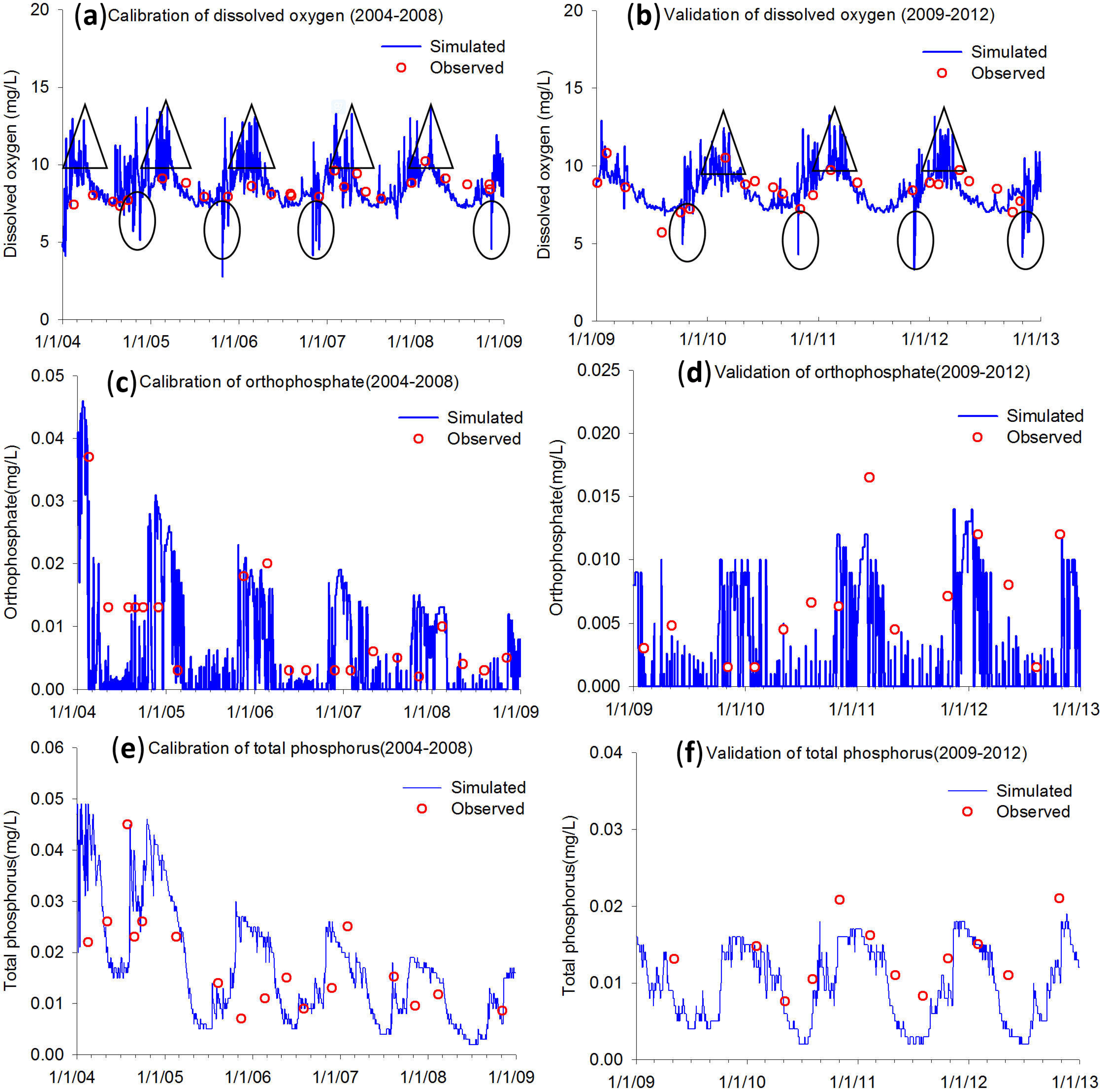
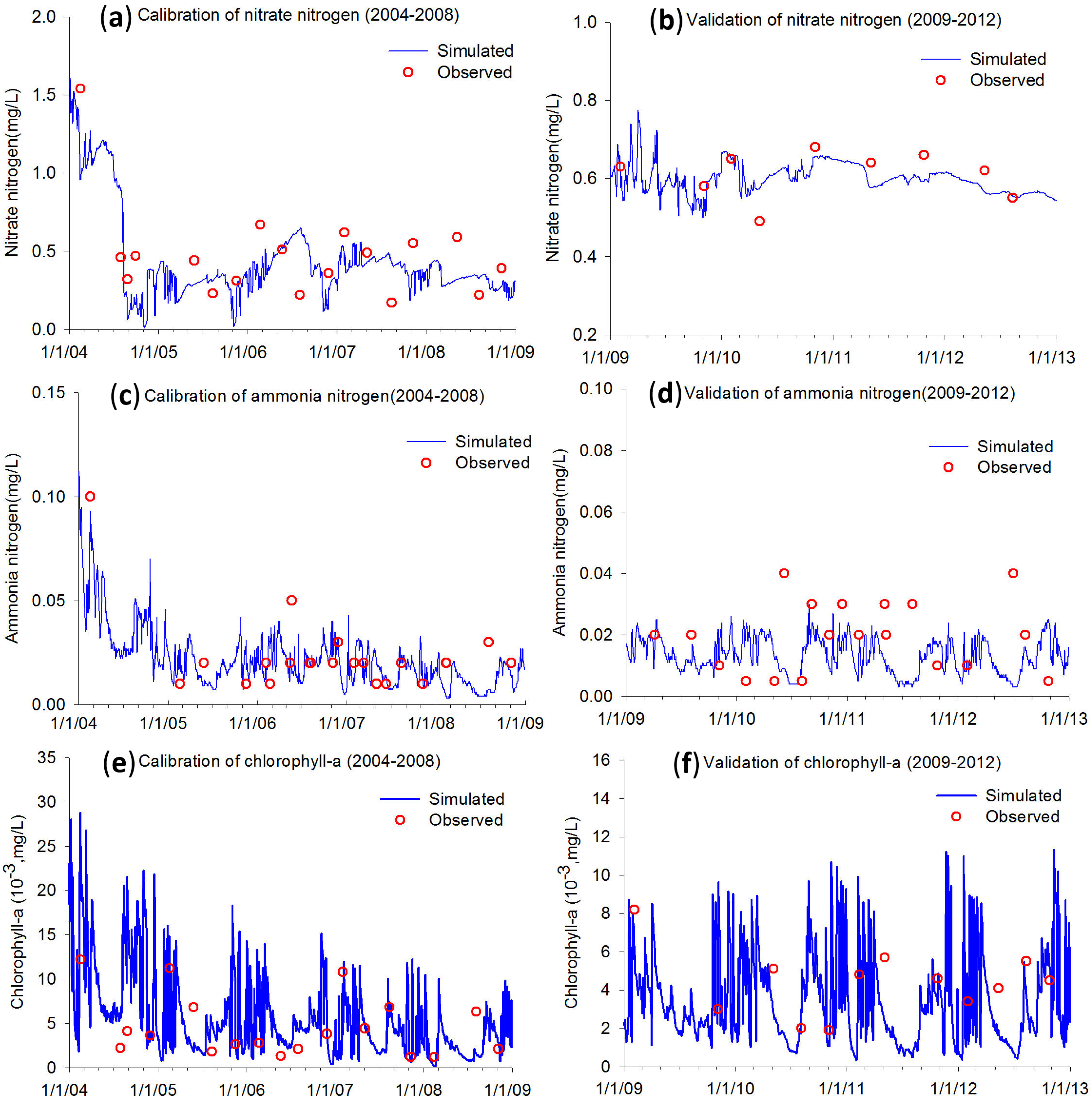
3.1. Calibration and Validation
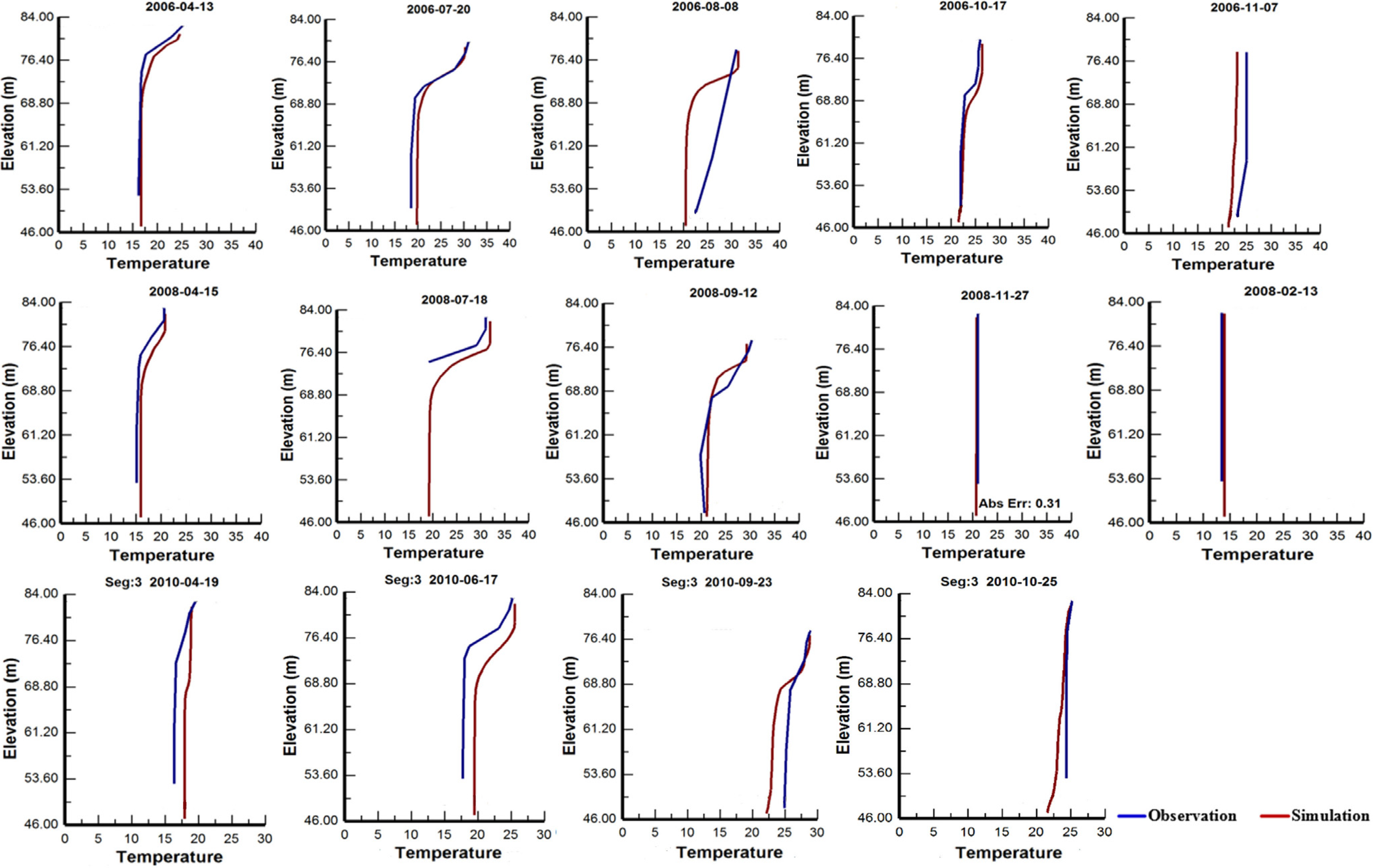
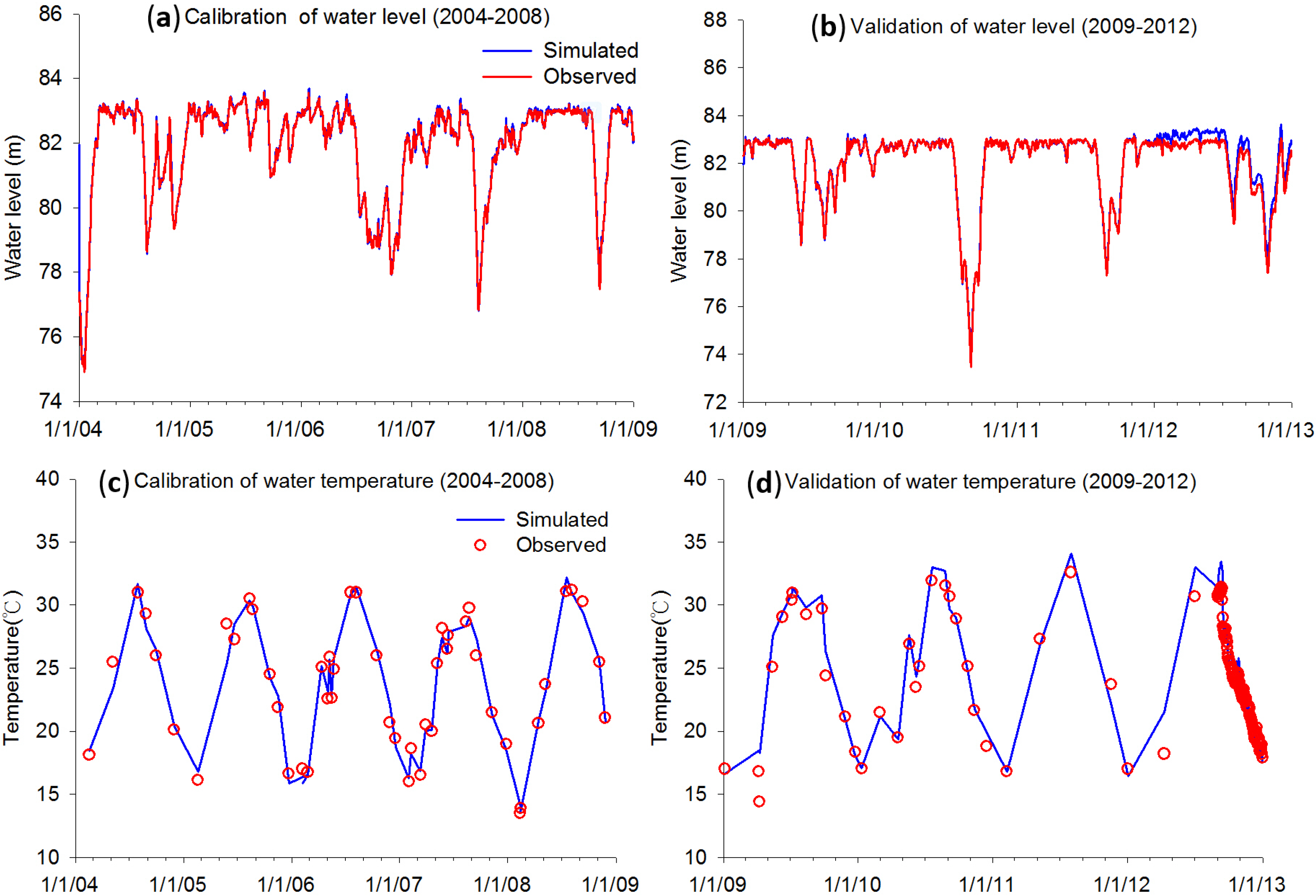
3.1.1. Hydrodynamic Variables
| Simulated Variables | Calibration | Validation | ||||||
|---|---|---|---|---|---|---|---|---|
| N | AME | RMSE | R2 | N | AME | RMSE | R2 | |
| Water level (m) | 1827 | 0.14 | 0.20 | 0.98 | 1460 | 0.13 | 0.15 | 0.99 |
| Surface temperature (°C) | 50 | 0.59 | - | 0.98 | 154 | 0.68 | - | 0.97 |
| DO (mg/L) | 27 | 0.72 | 0.94 | 0.49 | 30 | 1.12 | 1.49 | 0.26 |
| NH3–N (mg/L) | 22 | 0.019 | 0.025 | 0.51 | 16 | 0.021 | 0.026 | 0.25 |
| NO3–N (mg/L) | 22 | 0.172 | 0.212 | 0.32 | 16 | 0.348 | 0.371 | 0.37 |
| Ortho–P (mg/L) | 22 | 0.009 | 0.011 | 0.38 | 16 | 0.007 | 0.008 | 0.41 |
| TP (mg/L) | 22 | 0.009 | 0.012 | 0.49 | 16 | 0.01 | 0.012 | 0.49 |
| Chl-a (μg/L) | 22 | 2.752 | 3.689 | 0.32 | 16 | 2.186 | 2.919 | 0.36 |

3.1.2. Water Quality State Variables


3.2. Evaluating the Risks to Water Quality due to Climate Change
3.2.1. Water Temperature
| Parameter | Value | Ranking | Risk Exceedance Probability (%) | ||||
|---|---|---|---|---|---|---|---|
| 2004–2012 | 2020–2039 | 2080–2099 | |||||
| A1B | A2 | A1B | A2 | ||||
| Temperature (°C) | 18 | Low | 79.2 | 82.7 (81.1–84.2) | 81.8 (79.9–83.7) | 90.9 (89.6–92.1) | 90.8 (87.3–94.4) |
| 25 | Medium | 43.2 | 45.2 (43.9–46.6) | 44.8 (43.4–46.2) | 50.9 (49.4–52.5) | 51.5 (49.0–54.0) | |
| 32 | High | 9.4 | 11.8 (9.9–13.6) | 12.0 (11.1–12.9) | 18.6 (17.4–19.7) | 20.0 (16.7–23.2) | |
| DO (mg/L) | 6 | Low | 98.7 | 98.7 (98.6–98.8) | 98.7 (98.6–98.7) | 98.8 (98.7–98.8) | 98.8 (98.6–98.8) |
| 8.5 | Medium | 45.9 | 44.6 (43.5–45.6) | 45.2 (44.1–46.3) | 39.9 (38.1–41.7) | 39.8 (37.8–41.8) | |
| 11 | High | 6.3 | 6.3 (6.2–6.4) | 6.4 (6.2–6.5) | 5.9 (5.7–6.2) | 5.9 (5.5–6.3) | |
| Parameter | Period | Spring | Summer | Fall | Winter |
|---|---|---|---|---|---|
| Temperature (°C) | 2004–2012 | 3.13 | 10.84 | 6.59 | 0.62 |
| 2020–2039 | 3.16 | 10.85 | 6.62 | 0.62 | |
| 2080–2099 | 3.53 | 11.59 | 7.61 | 0.94 | |
| DO (mg/L) | 2004–2012 | 2.67 | 7.31 | 7.31 | 1.47 |
| 2020–2039 | 2.86 | 7.44 | 7.44 | 1.75 | |
| 2080–2099 | 3.38 | 7.7 | 7.7 | 2.6 |
3.2.2. DO
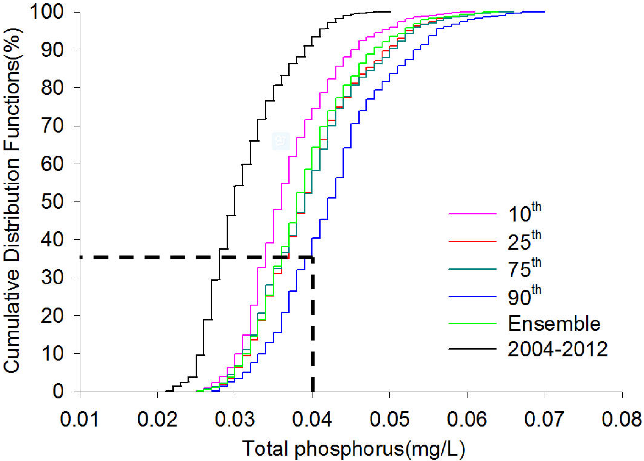
3.2.3. Nutrients
| Nutrient | Layer | Threshold (mg/L) | Ranking | Exceedance Probability (%) | ||||
|---|---|---|---|---|---|---|---|---|
| 2004–2012 | 2020–2039 | 2080–2099 | ||||||
| A1B | A2 | A1B | A2 | |||||
| PO43− | Surface | 0.015 | Low | 24.8 | 26.4 (26.0–26.8) | 26.4 (26.1–26.8) | 25.5 (25.1–25.9) | 25.1 (25.1–26.3) |
| 0.020 | Medium | 13.1 | 20.4 (19.0–21.7) | 20.7 (20.6–20.8) | 21.0 (20.5–21.4) | 20.8 (20.0–21.4) | ||
| 0.025 | High | 2.6 | 9.4 (6.7–12.0) | 7.9 (6.1–9.7) | 16.4 (15.0–17.9) | 15.9 (13.8–17.1) | ||
| Bottom | 0.015 | Low | 99.6 | 99.8 (99.7–99.8) | 99.8 (99.76–99.84) | 99.9 (99.8–99.9) | 99.9 (99.9–99.9) | |
| 0.020 | Medium | 92.0 | 96.2 (94.1–98.3) | 95.8 (94.4–97.3) | 98.0 (97.0–99.1) | 98.4 (98.2–98.5) | ||
| 0.025 | High | 49.8 | 71.8 (58.5–85.1) | 67.4 (58.3–76.5) | 89.9 (80.9–98.9) | 92.1 (89.8–94.3) | ||
| TP | Surface | 0.012 | Low | 81.6 | 85.7 (83.3–88.0) | 85.4 (82.6–88.3) | 93.8 (92.5–95.1) | 93.0 (91.3–94.7) |
| 0.024 | Medium | 38.6 | 48.6 (45.7–51.5) | 47.5 (44.7–50.2) | 55.5 (54.3–56.7) | 56.0 (53.7–58.4) | ||
| 0.035 | High | 4.7 | 9.1 (6.2–11.9) | 6.9 (5.6–8.2) | 22.3 (22.2–22.5) | 21.5 (14.8–25.7) | ||
| Bottom | 0.012 | Low | 100 | 100 (99.2–100) | 100 (98.5–100) | 100 (99.4–100) | 100 (99.1–100) | |
| 0.024 | Medium | 96.2 | 98.7 (97.4–100) | 98.3 (97.1–99.4) | 100 (99.3–100) | 100 (98.6–100) | ||
| 0.035 | High | 19.4 | 35.2 (23.3–47.0) | 29.6 (24.2–35.1) | 63.2 (42.4–84.0) | 65.4 (53.4–77.3) | ||
| Chl-a | Surface | 0.003 | Oligotrophic | 66.3 | 71.7 (70.3–73.1) | 71.3 (69.2–73.5) | 73.8 (72.8–74.7) | 75.3 (73.8–76.7) |
| 0.007 | Mesotrophic | 14.2 | 20.3 (17.9–22.6) | 18.9 (16.7–21.1) | 28.5 (27.9–29.1) | 28.4 (26.3–30.5) | ||
| 0.010 | Eutrophic | 2.7 | 5.4 (4.4–6.4) | 4.5 (3.6–5.4) | 9.8 (9.5–10.1) | 9.0 (7.4–10.6) | ||
| Nutrient | Layer | Threshold (mg/L) | Ranking | Exceedance Probability (%) | ||||
|---|---|---|---|---|---|---|---|---|
| 2004–2012 | 2020–2039 | 2080–2099 | ||||||
| A1B | A2 | A1B | A2 | |||||
| NH3–N | Surface | 0.01 | Low | 92.2 | 82.5 (81.4–83.5) | 82.5 (81.5–83.5) | 84.9 (83.8–86.0) | 85.7 (84.7–86.7) |
| 0.03 | Medium | 29.6 | 11.8 (9.4–14.3) | 10.6 (9.0–12.2) | 17.2 (14.2–20.3) | 17.6 (15.5–18.9) | ||
| 0.04 | High | 9.3 | 1.3 (1.1–1.5) | 1.2 (1.0–1.4) | 1.8 (1.3–2.4) | 1.7 (1.5–2.0) | ||
| Bottom | 0.01 | Low | 31.9 | 37.1 (33.8–40.4) | 36.5 (34.0–39.1) | 45.1 (41.3–48.9) | 47.3 (45.8–48.8) | |
| 0.03 | Medium | 6.7 | 9.1 (7.7–10.4) | 8.8 (7.5–10.1) | 14.6 (11.5–17.7) | 14.8 (12.5–17.1) | ||
| 0.04 | High | 5.1 | 6.7 (5.7–7.6) | 6.3 (5.3–7.4) | 10.2 (8.4–11.9) | 10.7 (9.5–11.9) | ||
| NO3–N | Surface | 0.2 | Low | 94.8 | 91.4 (89.9–93.0) | 91.9 (89.9–93.8) | 84.9 (83.3–86.6) | 82.8 (79.7–86.0) |
| 0.5 | Medium | 41.1 | 31.3 (29.4–33.2) | 31.2 (28.5–34.0) | 24.7 (23.1–26.3) | 23.9 (21.8–26.0) | ||
| 0.7 | High | 8.9 | 6.7 (6.3–7.2) | 6.8 (6.2–7.4) | 5.3 (5.0–5.7) | 5.2 (5.1–5.3) | ||
| Bottom | 0.2 | Low | 98.8 | 97.4 (96.3–98.5) | 97.7 (96.7–98.7) | 91.2 (87.9–94.5) | 90.6 (87.9–93.3) | |
| 0.5 | Medium | 61.7 | 56.7 (53.7–59.7) | 56.9 (53.5–60.3) | 45.3 (40.7–49.8) | 44.0 (39.2–48.9) | ||
| 0.7 | High | 17.3 | 12.7 (11.5–13.9) | 13.3 (11.5–15.1) | 10.3 (9.7–11.0) | 10.2 (9.5–10.9) | ||
3.2.4. Chlorophyll-a
4. Conclusions
Acknowledgments
Author Contributions
Conflicts of Interest
References
- Intergovernmental Panel on Climate Change (IPCC). Cimate Change 2007: The Physical Science Basis; Cambridge University Press: Cambridge, UK; New York, NY, USA, 2007; p. 996. [Google Scholar]
- Jones, J.; Brett, M.T. Lake nutrients, eutrophication, and climate change. In Global Environmental Change; Springer: New York, NY, USA, 2014; pp. 273–279. [Google Scholar]
- Intergovernmental Panel on Climate Change (IPCC). Managing the Risks of Extreme Events and Disasters to Advance Climate Change Adaptation; Cambridge University Press: Cambridge, UK; New York, NY, USA, 2012; p. 582. [Google Scholar]
- Huntington, T.G. Evidence for intensification of the global water cycle: Review and synthesis. J. Hydrol. 2006, 319, 83–95. [Google Scholar] [CrossRef]
- Stockholm International Water Institute (SIWI). The Role of Large Scale Artificial Water Storage in the Water-Food-Energy Development Nexus; SIWI: Stockholm, Sweden, 2009; p. 38. [Google Scholar]
- Deus, R.; Brito, D.; Mateus, M.; Kenov, I.; Fornaro, A.; Neves, R.; Alves, C. Impact evaluation of a pisciculture in the Tucuruí Reservoir (Pará, Brazil) using a two-dimensional water quality model. J. Hydrol. 2013, 487, 1–12. [Google Scholar] [CrossRef]
- Chung, S.; Oh, J. Calibration of CE-QUAL-W2 for a monomictic reservoir in a monsoon climate area. Water Sci. Technol. 2006, 54, 29–37. [Google Scholar] [CrossRef] [PubMed]
- Park, Y.; Cho, K.H.; Kang, J.-H.; Lee, S.W.; Kim, J.H. Developing a flow control strategy to reduce nutrient load in a reclaimed multi-reservoir system using a 2D hydrodynamic and water quality model. Sci. Total Environ. 2014, 466, 871–880. [Google Scholar] [CrossRef] [PubMed]
- Brooks, B.; Valenti, T.; Cook-Lindsay, B.; Forbes, M.; Doyle, R.; Scott, J.; Stanley, J. Influence of climate change on reservoir water quality assessment and management. In Climate; Springer: New York, NY, USA, 2011; pp. 491–522. [Google Scholar]
- Molina-Navarro, E.; Trolle, D.; Martínez-Pérez, S.; Sastre-Merlín, A.; Jeppesen, E. Hydrological and water quality impact assessment of a mediterranean limno-reservoir under climate change and land use management scenarios. J. Hydrol. 2014, 509, 354–366. [Google Scholar] [CrossRef]
- Varis, O.; Somlyody, L. Potential impacts of climate change on lake and reservoir water quality. In Water Resources Management in the Face of Climatic/Hydrologic Uncertainties; Kaczmarek, Z., Strzepek, K.M., Somlyódy, L., Priazhinskaya, V., Eds.; Kluwer Academic Publishers: Amsterdam, The Netherlands, 1996. [Google Scholar]
- Sahoo, G.; Schladow, S.; Reuter, J.; Coats, R. Effects of climate change on thermal properties of lakes and reservoirs, and possible implications. Stoch. Env. Res. Risk A 2011, 25, 445–456. [Google Scholar] [CrossRef]
- Duan, H.; Ma, R.; Xu, X.; Kong, F.; Zhang, S.; Kong, W.; Hao, J.; Shang, L. Two-decade reconstruction of algal blooms in China’s Lake Taihu. Environ. Sci. Technol. 2009, 43, 3522–3528. [Google Scholar] [CrossRef] [PubMed]
- Thorne, O.; Fenner, R. The impact of climate change on reservoir water quality and water treatment plant operations: A UK case study. Water Environ. J. 2011, 25, 74–87. [Google Scholar] [CrossRef]
- Zhu, M.; Zhu, G.; Zhao, L.; Yao, X.; Zhang, Y.; Gao, G.; Qin, B. Influence of algal bloom degradation on nutrient release at the sediment-water interface in Lake Taihu, China. Environ. Sci. Pollut. R. 2013, 20, 1803–1811. [Google Scholar] [CrossRef]
- Arheimer, B.; Andréasson, J.; Fogelberg, S.; Johnsson, H.; Pers, C.B.; Persson, K. Climate change impact on water quality: Model results from southern Sweden. AMBIO 2005, 34, 559–566. [Google Scholar] [PubMed]
- Trolle, D.; Hamilton, D.P.; Pilditch, C.A.; Duggan, I.C.; Jeppesen, E. Predicting the effects of climate change on trophic status of three morphologically varying lakes: Implications for lake restoration and management. Environ. Modell. Softw. 2011, 26, 354–370. [Google Scholar] [CrossRef]
- Carvalho, L.; Miller, C.; Spears, B.; Gunn, I.; Bennion, H.; Kirika, A.; May, L. Water quality of Loch Leven: Responses to enrichment, restoration and climate change. Hydrobiologia 2012, 681, 35–47. [Google Scholar] [CrossRef] [Green Version]
- Schindler, D.W.; Bayley, S.E.; Parker, B.R.; Beaty, K.G.; Cruikshank, D.R.; Fee, E.J.; Schindler, E.U.; Stainton, M.P. The effects of climatic warming on the properties of boreal lakes and streams at the experimental lakes area, northwestern Ontario. Limnol. Oceanogr. 1996, 41, 1004–1017. [Google Scholar] [CrossRef]
- Kim, B.; Park, J.-H.; Hwang, G.; Jun, M.-S.; Choi, K. Eutrophication of reservoirs in South Korea. Limnology 2001, 2, 223–229. [Google Scholar] [CrossRef]
- Jones, P.D.; New, M.; Parker, D.E.; Martin, S.; Rigor, I.G. Surface air temperature and its changes over the past 150 years. Rev. Geophys. 1999, 37, 173–199. [Google Scholar] [CrossRef]
- Shiu, C.-J.; Liu, S.C.; Chen, J.-P. Diurnally asymmetric trends of temperature, humidity, and precipitation in Taiwan. J. Clim. 2009, 22, 5635–5649. [Google Scholar] [CrossRef]
- Hsu, H.-H.; Chen, C.-T. Observed and projected climate change in Taiwan. Meteorol. Atmos. Phys. 2002, 79, 87–104. [Google Scholar] [CrossRef]
- Tseng, H.-W.; Yang, T.-C.; Kuo, C.-M.; Yu, P.-S. Application of multi-site weather generators for investigating wet and dry spell lengths under climate change: A case study in southern Taiwan. Water Resour. Manag. 2012, 26, 4311–4326. [Google Scholar] [CrossRef]
- Afshar, A.; Kazemi, H.; Saadatpour, M. Particle swarm optimization for automatic calibration of large scale water quality model (CE-QUAL-W2): Application to Karkheh Reservoir, Iran. Water Resour. Manag. 2011, 25, 2613–2632. [Google Scholar] [CrossRef]
- Cole, T.M.; Tillman, D.H. Water Quality Modeling of Lake Monroe Using CE-QUAL-W2; U.S. Army Engineer Waterways Experiment Station: Louisville, KY, USA, 1999; p. 94. [Google Scholar]
- Deus, R.; Brito, D.; Kenov, I.A.; Lima, M.; Costa, V.; Medeiros, A.; Neves, R.; Alves, C. Three-dimensional model for analysis of spatial and temporal patterns of phytoplankton in Tucuruí Reservoir, Pará, Brazil. Ecol. Model. 2013, 253, 28–43. [Google Scholar] [CrossRef]
- Giorgi, F.; Mearns, L.O. Calculation of average, uncertainty range, and reliability of regional climate changes from AOGCM simulations via the reliability ensemble averaging (REA) method. J. Clim. 2002, 15, 1141–1158. [Google Scholar] [CrossRef]
- Harding, B.; Wood, A.; Prairie, J. The implications of climate change scenario selection for future streamflow projection in the upper Colorado River Basin. Hydrol. Earth Syst. Sci. 2012, 9, 847–894. [Google Scholar] [CrossRef]
- Chiew, F.; Teng, J.; Vaze, J.; Post, D.; Perraud, J.; Kirono, D.; Viney, N. Estimating climate change impact on runoff across southeast Australia: Method, results, and implications of the modeling method. Water Resour. Res. 2009, 45. [Google Scholar] [CrossRef]
- Zhang, Y.; Wu, Z.; Liu, M.; He, J.; Shi, K.; Zhou, Y.; Wang, M.; Liu, X. Dissolved oxygen stratification and response to thermal structure and long-term climate change in a large and deep subtropical reservoir (Lake Qiandaohu, China). Water Res. 2015, 75, 249–258. [Google Scholar] [CrossRef] [PubMed]
- Wu, S.C.; Wu, J.T.; Chang, M.I. Correlation of Algae Eutrophication Indicators and Water Quality in Hsinshan Reservoir (2010); Taiwan Water Corporation: Taichung, Taiwan, 2010. (In Chinese) [Google Scholar]
- Cole, T.M.; Scott, A.W. CE-QUAL-W2: A Two-Dimensional, Laterally Averaged, Hydrodynamic and Water Quality Model; Version 3.71 User manual; U.S. Army Engineer Waterways Experiment Station: Louisville, KY, USA, 2013; p. 783. [Google Scholar]
- Mateus, M.; Almeida, C.; Brito, D.; Neves, R. From eutrophic to mesotrophic: Modelling watershed management scenarios to change the trophic status of a reservoir. Int. J. Environ. Res. Public Health 2014, 11, 3015–3031. [Google Scholar] [CrossRef] [PubMed]
- Debele, B.; Srinivasan, R.; Parlange, J.-Y. Coupling upland watershed and downstream waterbody hydrodynamic and water quality models (SWAT and CE-QUAL-W2) for better water resources management in complex river basins. Environ. Model. Assess. 2008, 13, 135–153. [Google Scholar] [CrossRef]
- Huang, Y.T.; Liu, L. A Hybrid perturbation and Morris approach for identifying sensitive parameters in surface water quality models. J. Environ. Inform. 2008, 12, 150–159. [Google Scholar] [CrossRef]
- Chang, C.H.; Wen, C.G.; Huang, C.H.; Chang, S.P.; Lee, C.S. Nonpoint source pollution loading from an undistributed tropic forest area. Environ. Monit. Assess. 2008, 146, 113–126. [Google Scholar] [CrossRef] [PubMed]
- Lee, C.S.; Chang, C.H.; Wen, C.G.; Chang, S.P. Comprehensive nonpoint source pollution models for a free-range chicken farm in a rural watershed in Taiwan. Agric. Ecosyst. Environ. 2010, 139, 23–32. [Google Scholar] [CrossRef]
- Wood, A.W.; Maurer, E.P.; Kumar, A.; Lettenmaier, D.P. Long-range experimental hydrologic forecasting for the eastern United States. J. Geophys. Res. Atmos. 2002, 107. [Google Scholar] [CrossRef]
- Chiew, F.; Kirono, D.; Kent, D.; Frost, A.; Charles, S.; Timbal, B.; Nguyen, K.; Fu, G. Comparison of runoff modelled using rainfall from different downscaling methods for historical and future climates. J. Hydrol. 2010, 387, 10–23. [Google Scholar] [CrossRef]
- Wetterhall, F.; Pappenberger, F.; He, Y.; Freer, J.; Cloke, H.L. Conditioning model output statistics of regional climate model precipitation on circulation patterns. Nonlinear Proc. Geoph. 2012, 19, 623–633. [Google Scholar] [CrossRef] [Green Version]
- Post, D.; Chiew, F.; Yang, A.; Viney, N.; Vaze, J.; Teng, J. The hydrologic impact of daily versus seasonal scaling of rainfall in climate change studies. In Interfacing Modelling and Simulation with Mathematical and Computational Sciences, Proceedings of the 18th World IMACS/MODSIM Congress, Cairns, Australia, 13–17 July 2009.
- Lin, L.-Y. A user-based climate change service project: Taiwan climate change projection and information platform project (TCCIP). In Proceedings of the 20th IHDP Scientific Committee Meeting, Taipei, Taiwan, 16–18 May 2013.
- Intergovernmental Panel on Climate Change (IPCC). Emissions Scenarios; Cambridge University Press: Cambridge, UK; New York, NY, USA, 2000. [Google Scholar]
- Environmental Protection Administration (EPA, Taiwan). The Environmental Water Quality Information System. Available online: http://wq.epa.gov.tw/WQEPA/Code/?Languages=en (accessed on 6 April 2015).
- Taiwan Environmental Analysis Laboratory. The Standard Methods for the Examination of Water and Wastewater. Available online: http://www.niea.gov.tw/ (accessed on 6 April 2015).
- Wu, S.C.; Wu, J.T.; Chang, M.I. Correlation of Algae Eutrophication Indicators and Water Quality in Hsinshan Reservoir (2011); Taiwan Water Corporation: Taichung, Taiwan, 2011. (In Chinese) [Google Scholar]
- Calson, R.E. A trophic state index for lakes. Limnol. Oceanogr. 1977, 22, 361–369. [Google Scholar] [CrossRef]
- Badran, M.I. Dissolved oxygen, chlorophyll a and nutrients: Seasonal cycles in waters of the Gulf of Aquaba, Red Sea. Aquat. Ecosyst. Health 2001, 4, 139–150. [Google Scholar] [CrossRef]
- Martin, S.C.; Effler, S.W.; DePinto, J.V.; Trama, F.B.; Rodgers, P.W.; Dobi, J.S.; Wodka, M.C. Dissolved oxygen model for a dynamic reservoir. J. Environ. Eng. ASCE 1985, 111, 647–664. [Google Scholar] [CrossRef]
- Carpenter, S.R. Phosphorus control is critical to mitigating eutrophication. Proc. Natl. Acad. Sci. USA 2008, 105, 11039–11040. [Google Scholar] [CrossRef] [PubMed]
- Lindenschmidt, K.E.; Fleischbein, K.; Baborowski, M. Structural uncertainty in a river water quality modelling system. Ecolog. Model. 2007, 204, 289–300. [Google Scholar] [CrossRef]
- Kay, A.L.; Davies, H.N.; Bell, V.A.; Jones, R.G. Comparison of uncertainty sources for climate change impacts: flood frequency in England. Clim. Change 2009, 92, 41–63. [Google Scholar] [CrossRef] [Green Version]
- Horton, P.; Schaefli, B.; Mezghani, A.; Hingray, B.; Musy, A. Assessment of climate-change impacts on alpine discharge regimes with climate model uncertainty. Hydrol. Process 2006, 20, 2091–2109. [Google Scholar] [CrossRef]
- Wilby, R. L.; Harris, I. A framework for assessing uncertainties in climate change impacts: Low-flow scenarios for the River Thames, UK. Water Resour. Res. 2006, 42. [Google Scholar] [CrossRef]
- Kanoshina, I.; Lips, U.; Leppänen, J.-M. The influence of weather conditions (temperature and wind) on cyanobacterial bloom development in the Gulf of Finland (Baltic Sea). Harmful Algae 2003, 2, 29–41. [Google Scholar] [CrossRef]
- Foley, B.; Jones, I.D.; Maberly, S.C.; Rippey, B. Long-term changes in oxygen depletion in a small temperate lake: Effects of climate change and eutrophication. Freshwater Biol. 2012, 57, 278–289. [Google Scholar] [CrossRef]
- Bates, B.C.; Kundzewicz, Z.W.; Wu, S.; Palutikof, J.P. Climate change and water. In Technical Paper of the Intergovernmental Panel on Climate Change; Intergovernmental Panel on Climate Change (IPCC): Geneva, Switzerland, 2008; p. 210. [Google Scholar]
- Nikolai, S.J.; Dzialowski, A.R. Effects of internal phosphorus loading on nutrient limitation in a eutrophic reservoir. Limnologica 2014, 49, 33–41. [Google Scholar] [CrossRef]
- Robarts, R.D.; Zohary, T. Temperature effects on photosynthetic capacity, respiration, and growth rates of bloom-forming cyanobacteria. N. Z. J. Mar. Freshwater Res. 1987, 21, 391–399. [Google Scholar] [CrossRef]
- Huang, J.C.; Gao, J.F.; Mooij, W.M.; Hörmann, G.; Fohrer, N. A comparison of three Approaches to predict phytoplankton biomass in Gonghu Bay of Lake Taihu. J. Environ. Inform. 2014, 24, 39–51. [Google Scholar]
- Singleton, V.L.; Little, J.C. Designing hypolimnetic aeration and oxygenation systems—A review. Environ. Sci. Technol. 2006, 40, 7512–7520. [Google Scholar] [CrossRef] [PubMed]
© 2015 by the authors; licensee MDPI, Basel, Switzerland. This article is an open access article distributed under the terms and conditions of the Creative Commons Attribution license (http://creativecommons.org/licenses/by/4.0/).
Share and Cite
Chang, C.-H.; Cai, L.-Y.; Lin, T.-F.; Chung, C.-L.; Van der Linden, L.; Burch, M. Assessment of the Impacts of Climate Change on the Water Quality of a Small Deep Reservoir in a Humid-Subtropical Climatic Region. Water 2015, 7, 1687-1711. https://doi.org/10.3390/w7041687
Chang C-H, Cai L-Y, Lin T-F, Chung C-L, Van der Linden L, Burch M. Assessment of the Impacts of Climate Change on the Water Quality of a Small Deep Reservoir in a Humid-Subtropical Climatic Region. Water. 2015; 7(4):1687-1711. https://doi.org/10.3390/w7041687
Chicago/Turabian StyleChang, Chih-Hua, Long-Yan Cai, Tsair-Fuh Lin, Chia-Ling Chung, Leon Van der Linden, and Michael Burch. 2015. "Assessment of the Impacts of Climate Change on the Water Quality of a Small Deep Reservoir in a Humid-Subtropical Climatic Region" Water 7, no. 4: 1687-1711. https://doi.org/10.3390/w7041687