Predicting Multiple Functions of Sustainable Flood Retention Basins under Uncertainty via Multi-Instance Multi-Label Learning

Abstract

The ambiguity of diverse functions of sustainable flood retention basins (SFRBs) may lead to conflict and risk in water resources planning and management. How can someone provide an intuitive yet efficient strategy to uncover and distinguish the multiple potential functions of SFRBs under uncertainty? In this study, by exploiting both input and output uncertainties of SFRBs, the authors developed a new data-driven framework to automatically predict the multiple functions of SFRBs by using multi-instance multi-label (MIML) learning. A total of 372 sustainable flood retention basins, characterized by 40 variables associated with confidence levels, were surveyed in Scotland, UK. A Gaussian model with Monte Carlo sampling was used to capture the variability of variables (i.e., input uncertainty), and the MIML-support vector machine (SVM) algorithm was subsequently applied to predict the potential functions of SFRBs that have not yet been assessed, allowing for one basin belonging to different types (i.e., output uncertainty). Experiments demonstrated that the proposed approach enables effective automatic prediction of the potential functions of SFRBs (e.g., accuracy >93%). The findings suggest that the functional uncertainty of SFRBs under investigation can be better assessed in a more comprehensive and cost-effective way, and the proposed data-driven approach provides a promising method of doing so for water resources management.

1. Introduction

There is a wide range of natural watercourses and traditional engineering solutions that can be applied for flood protection in urban and rural areas, such as barriers and dykes. The concept of sustainability has recently been introduced to flood defenses [1]. As an adaptive structural measure, sustainable flood retention basins (SFRBs) have been proposed to facilitate the implementation of the Flood Directive [2,3]. An SFRB is internationally defined as a natural or artificial impoundment or integrated wetland, which has a pre-defined or potential role in flood defense and diffuse pollution control that can be accomplished cost-effectively through best management practices, achieving sustainable flood risk management and enhancing sustainable drainage, pollution reduction, biodiversity, green space, and recreational opportunities for society [4]. In reality, different SFRBs usually perform diverse functions such as flood control, irrigation, drinking water supply and electricity generation. Ambiguity between these functions may lead to conflict or risk for decision-makers in charge of water resources management and planning. Therefore, methods to assess and distinguish the functions of water bodies have been attracting increased attention in the field of water resources research.

During past decades, many typological approaches for various kinds of water bodies have been proposed [5,6,7,8]. For instance, the Ramsar classification system [9] divides wetlands into three main categories (i.e., marine and coastal wetlands, inland wetlands and man-made wetlands) and 43 associated wetland types. This classification system is complicated and requires detailed data sets that are frequently not available. The system also does not show direct relationships between the types and diverse functions of water bodies.

In the United States, a hierarchical classification system has been proposed for wetlands and deep water habitats [5]. The highest level consists of five classes (Marine, Estuarine, Riverine, Lacustrine, and Palustrine), and each class has different sub-classes. This classification scheme also hardly considers the functions of water bodies.

Under the European Water Framework Directive [10], a classification scheme for surface water bodies has been established by incorporating ecological status and chemical status classification [11]. However, the monitoring program is mainly based on biological and chemical elements and is extremely time-consuming and costly. Moreover, the classification system assesses the status of water bodies instead of the functions of water bodies.

In Florida, surface waters are classified into six types. Designated uses and water quality criteria were established for each type [12]. However, this functional assessment of water bodies is mainly based on water quality rather than comprehensive properties. Therefore, to better assess and distinguish the functions of a large number of basins, a rapid and efficient classification method based on comprehensive properties is greatly needed.

One strategy is to build a data-driven environmental model. The basic idea is to first collect and integrate different types of data to characterize the system under study, and then apply pattern classification approaches such as a support vector machine [13], artificial neural networks [14], a self-organizing map [15,16] and multi-label classification [17] to solve real, practical problems. Recently, to handle the input and output ambiguity, Zhou and Zhang [18] further proposed multi-instance multi-label learning for image classification, which performs well compared to traditional pattern classification or multi-instance learning or multi-label learning. Therefore, in this study, to capture the ambiguities of SFRBs from aspects of input and output, the team investigates them using multi-instance multi-label learning.

According to the practical functions, six types of SFRBs based on various indicators are defined by different professions [2]. Uncertainty is one of the most challenging problems in SFRB system analysis, and here the authors focus on its associated input and output uncertainty. Input uncertainty mainly originates from estimation bias and measurement error concerning some SFRB properties during rapid data acquisition. For output, one basin usually has multiple potential functions and satisfies multiple demands and thus belongs to multiple types. As a result, output uncertainty is here regarded as ambiguity in type determination for SFRBs. Function uncertainty caused by hydrological uncertainty is out of the scope of this paper. To gain deeper insight into the multiple functions of SFRBs, in this study, the authors investigate the input and output uncertainties of basins simultaneously.

In recent years, many studies have focused on uncertainty analysis of water resources, specifically for water resources management and planning [19,20,21], hydrologic modeling [22,23], distributed watershed modeling [24], decision making [25,26], water allocation [27,28], and water quality [29]. Various uncertainty analysis techniques have been developed. For instance, regression, Monte Carlo analysis, multiple modeling and the moment equation approach are all strategies for uncertainty analysis applied in ground water modeling [30]. For watershed modeling, five uncertainty analysis techniques are widely used: Generalized Likelihood Uncertainty Estimation (GLUE) [31], Parameter Solution (ParaSol) [32], the Sequential Uncertainty Fitting algorithm (SUFI-2) [33], and a Bayesian framework implemented using Markov Chain Monte Carlo (MCMC) and Importance Sampling (IS) techniques [34]. Furthermore, a framework and guide for uncertainty in the environmental modeling process has been proposed, and 14 uncertainty assessment methods were reviewed [35]. Different techniques with different concepts give users some freedom to formulate functions as required. However, most of the abovementioned work concentrated on model structure and parameter uncertainties, while the input and output uncertainties of water bodies were of less concern [36,37].

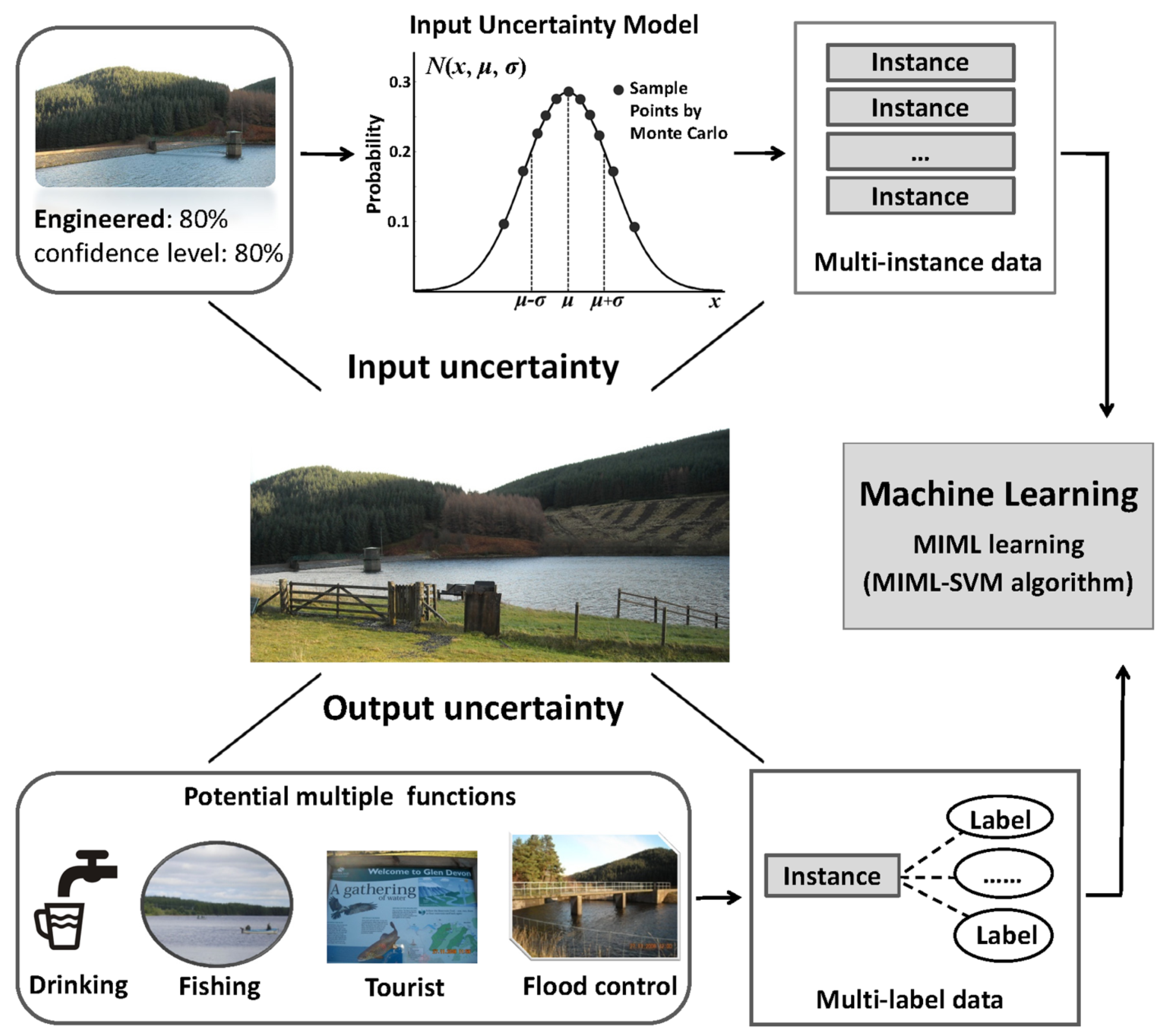
In this paper, the authors propose a new data-driven framework to optimize the multi-criteria analysis of SFRBs with uncertainty. The objective of this study is to identify potential multiple functions of water bodies under uncertainty by using multi-instance multi-label learning. In detail, to characterize the intrinsic properties of water bodies, a Gaussian model with Monte Carlo sampling is used to capture its input data uncertainty. Thereafter, one basin is represented by multiple instances. To further investigate the functional ambiguity of water bodies (output uncertainty), the MIML-SVM algorithm has been applied to automatically predict the potential functions of SFRBs that have not yet been assessed.

2. Methodology

2.1. Data Acquisition

In Scotland, there is a high number of water bodies with diverse functions. The sites of interest are those where the water level can be controlled either manually or automatically. In total, 372 SFRBs situated in central Scotland have been selected and surveyed in this study (Figure 1). To characterize the properties of water bodies, 40 variables (see Table 1) were proposed based on a literature review and field experience [38]. 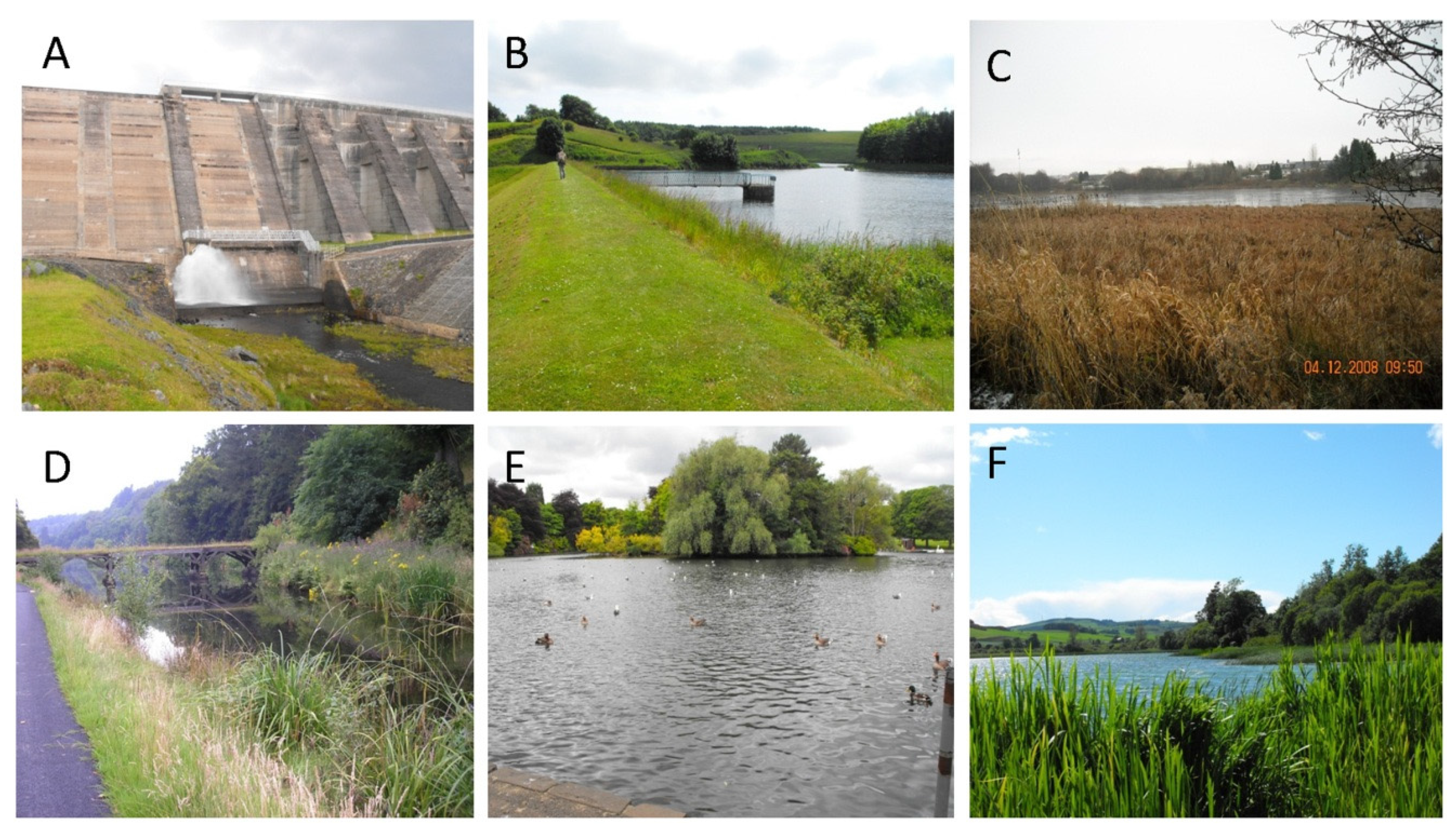To analyze the functions of SFRBs, based on international expert judgment, empirical studies, statistical analysis and feedback from collaborators, six SFRB types were defined [39]. Namely, hydraulic flood retention basins (Type 1, Figure 2A), traditional flood retention basins (Type 2, Figure 2B), sustainable flood retention wetland (Type 3, Figure 2C), aesthetic flood treatment wetland (Type 4, Figure 2D), integrated flood retention wetland (Type 5, Figure 2E) and natural flood retention wetland (Type 6, Figure 2F). In addition, Table 2 shows the relationships among SFRB types, dominant functions of SFRBs, and the typical examples of each type of SFRB.

Figure 1. Map of 372 identified sustainable flood retention basins (SFRBs) in the wider Central Scotland area (UK).

Figure 1. Map of 372 identified sustainable flood retention basins (SFRBs) in the wider Central Scotland area (UK).

Table 1. Classification variables used for the assessment of sustainable flood retention basins.

ID	Variable and Unit	ID	Variable and Unit
1	Engineered (%)	21	Impermeable Soil Proportion (%)
2	Dam Height (m)	22	Seasonal Influence (%)
3	Dam Length (m)	23	Site Elevation (m)
4	Outlet Arrangement and Operation (%)	24	Vegetation Cover (%)
5	Aquatic Animal Passage (%)	25	Algal Cover in Summer (%)
6	Land Animal Passage (%)	26	Relative Total Pollution (%)
7	Floodplain Elevation (m)	27	Mean Sediment Depth (cm)
8	Basin and Channel Connectivity (m)	28	Organic Sediment Proportion (%)
9	Wetness (%)	29	Flotsam Cover (%)
10	Proportion of Flow within Channel (%)	30	Catchment Size (km2)
11	Mean Flooding Depth (m)	31	Urban Catchment Proportion (%)
12	Typical Wetness Duration (day/year)	32	Arable Catchment Proportion (%)
13	Estimated Flood Duration (day/year)	33	Pasture Catchment Proportion (%)
14	Basin Bed Gradient (%)	34	Viniculture Catchment Proportion (%)
15	Mean Basin Flood Velocity (cm/s)	35	Forest Catchment Proportion (%)
16	Wetted Perimeter (m)	36	Natural Catchment Proportion (%)
17	Maximum Flood Water Volume (m3)	37	Groundwater Infiltration (%)
18	Flood Water Surface Area (m2)	38	Mean Depth of the Basin (m)
19	Mean Annual Rainfall (mm)	39	Length of Basin (m)
20	Drainage (cm/day)	40	Width of Basin (m)

Table 1. Classification variables used for the assessment of sustainable flood retention basins.

ID	Variable and Unit	ID	Variable and Unit
1	Engineered (%)	21	Impermeable Soil Proportion (%)
2	Dam Height (m)	22	Seasonal Influence (%)
3	Dam Length (m)	23	Site Elevation (m)
4	Outlet Arrangement and Operation (%)	24	Vegetation Cover (%)
5	Aquatic Animal Passage (%)	25	Algal Cover in Summer (%)
6	Land Animal Passage (%)	26	Relative Total Pollution (%)
7	Floodplain Elevation (m)	27	Mean Sediment Depth (cm)
8	Basin and Channel Connectivity (m)	28	Organic Sediment Proportion (%)
9	Wetness (%)	29	Flotsam Cover (%)
10	Proportion of Flow within Channel (%)	30	Catchment Size (km2)
11	Mean Flooding Depth (m)	31	Urban Catchment Proportion (%)
12	Typical Wetness Duration (day/year)	32	Arable Catchment Proportion (%)
13	Estimated Flood Duration (day/year)	33	Pasture Catchment Proportion (%)
14	Basin Bed Gradient (%)	34	Viniculture Catchment Proportion (%)
15	Mean Basin Flood Velocity (cm/s)	35	Forest Catchment Proportion (%)
16	Wetted Perimeter (m)	36	Natural Catchment Proportion (%)
17	Maximum Flood Water Volume (m3)	37	Groundwater Infiltration (%)
18	Flood Water Surface Area (m2)	38	Mean Depth of the Basin (m)
19	Mean Annual Rainfall (mm)	39	Length of Basin (m)
20	Drainage (cm/day)	40	Width of Basin (m)

Figure 2. Typical examples for six different types of sustainable flood retention basins. (A): Hydraulic Flood Retention Basin; (B): Traditional Flood Retention Basin; (C): Sustainable Flood Retention Wetland; (D): Aesthetic Flood Treatment Wetland; (E): Integrated Flood Retention Wetland; (F): Natural Flood Retention Wetland.

Figure 2. Typical examples for six different types of sustainable flood retention basins. (A): Hydraulic Flood Retention Basin; (B): Traditional Flood Retention Basin; (C): Sustainable Flood Retention Wetland; (D): Aesthetic Flood Treatment Wetland; (E): Integrated Flood Retention Wetland; (F): Natural Flood Retention Wetland.

Table 2. The relationships among sustainable flood retention basin types and functions.

SFRB Type	Type Name	Dominant Function	Typical Examples
1	Hydraulic Flood Retention Basin (HFRB)	Hydroelectricity generation and drinking water supply	Hydropower reservoir; highly engineered and large-scale drinking water reservoir (Figure 2A)
2	Traditional Flood Retention Basin (TFRB)	Flood control	Former drinking water reservoir; traditional flood retention basin (Figure 2B)
3	Sustainable Flood Retention Wetland (SFRW)	Retention and drainage	Sustainable drainage systems or best management practices such as some retention and detention basins (Figure 2C)
4	Aesthetic Flood Treatment Wetland (AFTW)	Integrated floodwater treatment	Some modern constructed treatment wetlands and integrated constructed wetlands (Figure 2D)
5	Integrated Flood Retention Wetland (IFRW)	Multiple recreation functions (e.g., fishing, water sports)	Some artificial water bodies within parks or near motorways; Reservoirs providing recreational activities (Figure 2E)
6	Natural Flood Retention Wetland (NFRW)	Nature conservation	Natural or semi-natural lakes and large ponds, potentially with restricted access (Figure 2F)

Table 2. The relationships among sustainable flood retention basin types and functions.

SFRB Type	Type Name	Dominant Function	Typical Examples
1	Hydraulic Flood Retention Basin (HFRB)	Hydroelectricity generation and drinking water supply	Hydropower reservoir; highly engineered and large-scale drinking water reservoir (Figure 2A)
2	Traditional Flood Retention Basin (TFRB)	Flood control	Former drinking water reservoir; traditional flood retention basin (Figure 2B)
3	Sustainable Flood Retention Wetland (SFRW)	Retention and drainage	Sustainable drainage systems or best management practices such as some retention and detention basins (Figure 2C)
4	Aesthetic Flood Treatment Wetland (AFTW)	Integrated floodwater treatment	Some modern constructed treatment wetlands and integrated constructed wetlands (Figure 2D)
5	Integrated Flood Retention Wetland (IFRW)	Multiple recreation functions (e.g., fishing, water sports)	Some artificial water bodies within parks or near motorways; Reservoirs providing recreational activities (Figure 2E)
6	Natural Flood Retention Wetland (NFRW)	Nature conservation	Natural or semi-natural lakes and large ponds, potentially with restricted access (Figure 2F)

The data collection for each SFRB consisted of a two-stage process: a desk study and a field visit. The desk study (each site usually takes 30 to 60 min) provided a rapid estimate of most variables by checking information from the Scottish Flood Defense Asset Database [40], digital maps and relevant regional references such as the Meteorological Office and the Scottish Environment Protection Agency [41]. For instance, during the desk study, the catchment size, land use types in the catchment (urban, arable, forestry and natural grassland proportion), wetted perimeter, length of the dam and elevation could be measured using 1:50,000 or 1:25,000 digital maps.

The field visit was conducted to verify the attributes determined during the desk study. Each visit required three to five experts to attend. With the agreement of all experts, data for 40 characteristic variables and functions of SFRB were recorded. The photographic records of water body inflows and outflows are documented. For more details of how to rapidly survey a water body, please refer to the published guidance [38].

In this study, due to environmental and human factors, the estimation or measurement of each variable is usually not 100% accurate. For instance, the variable “Engineered” determines whether the SFRB is natural or man-made and how pronounced these tendencies are. The estimation depends greatly on the experts’ knowledge. Dam structures with full engineering control such as a modern drinking water supply reservoir or a hydraulic flood retention basin would typically receive values of between 70% and 95%. The variable “Vegetation Cover” can only be estimated but not measured accurately. Dry SFRB covered by short grass can achieve a vegetation cover value between 20% and 70%, while mature vegetation such as a full basin covered with trees is associated with a value close to 100%. Even for the measured data, inherent errors exist despite following strict quality assurance and quality control guidelines [31]. To quantify the input data uncertainty, during data collection, a confidence level (i.e., Low: 1% to 40%; Medium: 40% to 60%; High: 60% to 100%) was introduced and attributed to each variable to reflect how confident the assessors were of their estimations. Data with low confidence levels were subsequently improved by a further literature review or a follow-up field visit.

2.2. Evaluation of Uncertainty

To assess the multiple functions of SFRBs, in this study, the team proposes a data-driven framework, which is simply illustrated in Figure 3. To deal with the input uncertainty, the authors use a Gaussian model and Monte Carlo sampling technique to capture the variability of each variable. Following that, each water body is represented by multiple instances. To further assess the ambiguity of SFRB functions, the MIML-SVM algorithm is applied to automatically identify the potential multiple types of water bodies.

Figure 3. Schema of the proposed framework.

Figure 3. Schema of the proposed framework.

2.2.1. Evaluation of Input Uncertainty

To objectively represent the status of the SFRB to some extent, a confidence level is assigned to each variable data point. However, uncertainty still remains and makes it difficult to know the true values of SFRB properties. An interesting question is as follows: how can one integrate the confidence level into SFRB analysis so as to get closer to the intrinsic properties of the SFRB? For this purpose, the team proposes a simple yet effective model to determine the input data uncertainty originating from data acquisition (see Section 2.1).

The basic idea is intuitive. The authors use a set of values sampled from a Gaussian distribution using the Monte Carlo method to represent each variable of each SFRB, instead of the original single value. The rationale is that if the acquired value of one variable associated with an SFRB is associated with a high confidence level, the potential true value is expected to be closer to its current value and falls into a relatively narrow range around it, and vice versa. In such a situation, the mean and standard deviation parameters denote the acquired value and the variability estimated with confidence levels, respectively.

One can generate a number of values according to the corresponding Gaussian probability distribution with Monte Carlo sampling. Formally, let x_i be one sample of SFRB data, and x_ij be the j-th variable of the sample x_i, a set of values (K) following the Gaussian probability distribution function N (x, μ, σ) (Equation (1)) are generated to represent each variable x_ij.

$$N\left(x,\text{μ},\text{σ}\right)=\frac{1}{\sigma \sqrt{2\text{π}}}{e}^{-\frac{{\left(x-\text{μ}\right)}^2}{2{\text{σ}}^2}}$$

(1)

The expected value μ is the original data of each variable, and the standard deviation σ of the Gaussian distribution function is defined in Equation (2).

$$\text{σ}={\left(1-\text{α}\right)}^{\text{β}}\cdot std$$

(2)

where α is the confidence level, β is the control factor and a positive constant, and std indicates the standard deviation value of the j-th variable in the original data (Equation (3)).

$$std=\sqrt{\frac{1}{N}{\displaystyle \sum }_{i=1}^N{(x_{ij}-\overline{x_j})}^2}$$

(3)

where N is the total number of SFRB samples, $\overline{x_j}$ presents the average value of each variable, which is calculated in Equation (4).

$$\overline{x_j}=\frac{1}{N}{\displaystyle \sum }_{i=1}^N{x}_{ij}$$

(4)

According to the uncertainty model, each sample can be represented by a set of instances sampled from a Gaussian distribution, which is denoted as X_i = {X_i¹, X_i²,…, X_i^K}. Hence, the variability or uncertainties of the variables of each SFRB are well-modeled by a set of values, which provides a potential way to capture the real and intrinsic properties of input data in an intuitive and effective fashion. Namely, the true value of each variable is well-estimated by a set of values instead of a single potential error (bias) value.

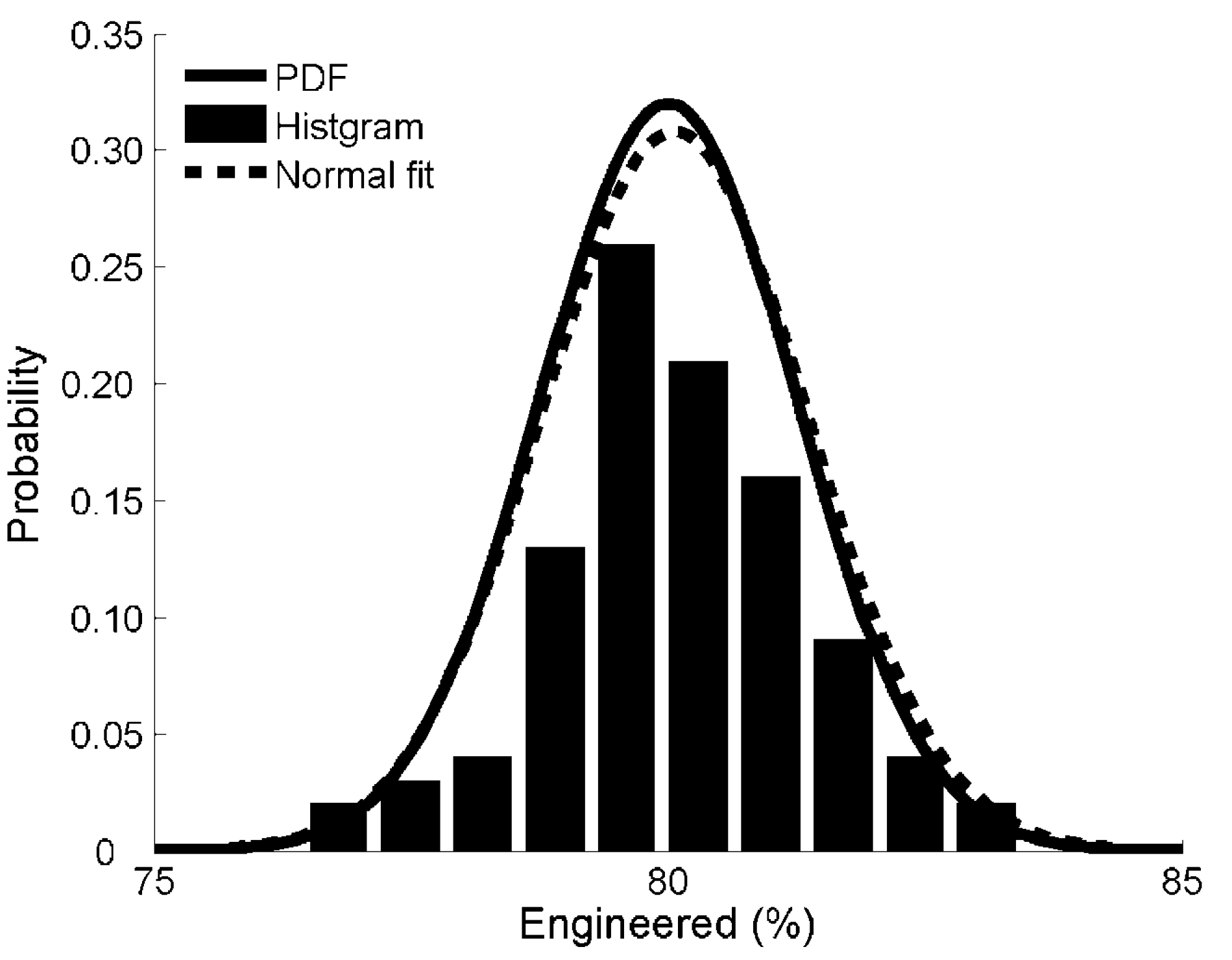
To illustrate this, take Glensherup Reservoir (56°7'48'' N, 3°24'3'' W; The reservoir example shown in Figure 3). Table 3 gives the thirty instances that were generated followed by the Gaussian distribution function according to its confidence levels. Figure 4 further plots the distribution of the first variable (“Engineered”) on the newly generated data based on the uncertainty model. One can observe that the set generated values fit Gaussian (Normal) distribution well, and provide a good way to estimate the true value of “Engineered” with different probabilities.

Table 3. The generated new data based on the uncertainty model (taking Glensherup Reservoir (Figure 3) as a representative example).

Variable	Engineered (%)	Dam Height (m)	Dam Length (m)	Outlet Operation (%)	Width of Basin (m)
Xi	80.00	20.00	250.00	75.00	200.00
C.l.	0.80	0.70	0.80	0.85	0.90
σ	1.25	0.81	7.54	0.71	2.63
Xi1	80.02	19.34	250.34	74.50	200.24
Xi2	80.55	19.99	249.71	75.26	202.46
Xi3	79.82	20.26	250.50	75.05	200.29
Xi4	79.87	20.09	244.95	74.94	201.56
Xi5	81.23	20.32	248.35	75.30	199.40
XiK	79.80	20.08	250.55	75.37	198.02

Notes: X_i: Original data; and C.l.: Confidence level.

Table 3. The generated new data based on the uncertainty model (taking Glensherup Reservoir (Figure 3) as a representative example).

Variable	Engineered (%)	Dam Height (m)	Dam Length (m)	Outlet Operation (%)	Width of Basin (m)
Xi	80.00	20.00	250.00	75.00	200.00
C.l.	0.80	0.70	0.80	0.85	0.90
σ	1.25	0.81	7.54	0.71	2.63
Xi1	80.02	19.34	250.34	74.50	200.24
Xi2	80.55	19.99	249.71	75.26	202.46
Xi3	79.82	20.26	250.50	75.05	200.29
Xi4	79.87	20.09	244.95	74.94	201.56
Xi5	81.23	20.32	248.35	75.30	199.40
XiK	79.80	20.08	250.55	75.37	198.02

Notes: X_i: Original data; and C.l.: Confidence level.

Figure 4. The histogram of the newly generated data for the variable “Engineered” (%) for Glensherup Reservoir based on the uncertainty model (μ = 80, σ = 1.25 and K = 100); Normal fit (μ' = 80.06 and σ' = 1.29); PDF, probability density function.

Figure 4. The histogram of the newly generated data for the variable “Engineered” (%) for Glensherup Reservoir based on the uncertainty model (μ = 80, σ = 1.25 and K = 100); Normal fit (μ' = 80.06 and σ' = 1.29); PDF, probability density function.

In this study, the authors model and encode the potential true values using the set of values, which allows for the provision of more accurate information to assess the multiple functions of water bodies. As each SFRB is represented as a set of values with uncertainty (input uncertainty) and it usually performs multiple functions and is associated with multiple SFRB types (output uncertainty), the task of multi-label classification of water bodies is naturally transferred into a multi-instance multi-label learning problem.

2.2.2. Evaluation of Output Uncertainty

2.2.2.1. Preliminaries

In traditional supervised learning, an object is represented as one instance and associated with only one class label. The task is to learn a function l = f(x) from a given data set D = {(x₁, l₁), (x₂, l₂), ..., (x_m, l_m)}, where $x_i\in x$ is an example and $l_i\in l$ is the corresponding label.

For multi-instance learning, each example associated with one label is represented by several instances. The goal is to find a function l = f(x) from a given data set D = {(x₁, l₁), (x₂, l₂), ..., (x_m, l_m)}, where $X_i=\left\{x_i^1, x_i^1, \dots , x_i^{ni}\right\}$ is a set of instances (e.g., X_i is the set of instances generated by the uncertainty model in this study), ni is the number of corresponding instances and $l_i\in l$ is its label.

In contrast, multi-label learning studies the problem where an example described by one instance is associated with multiple labels. Formally, the task is to gain knowledge of a function L = f(x) from a given data set D = {(x₁, l₁), (x₂, l₂), ..., (x_m, l_m)}, where x_i $\in$ x is an example, $L_i=\left\{l_i^1, l_i^2, \dots , l_i^{li}\right\}$ is a set of labels (e.g., L_i is the multiple types of one SFRB), l_i is the number of labels of the example and $l_i\in l$ is the corresponding label.

However, the multi-instance or multi-label frameworks cannot capture all real-world problems. For example, take an image containing many regions represented as many instances, and belonging to multiple semantic classes. Therefore, a more complicated problem is to determine a function L = f(X) from a given data set D = {(X₁, L₁), (X₂, L₂), ..., (X_m, L_m)}, where X_i is represented by a set of instances $\left\{x_i^1, x_i^1, \dots , x_i^{ni}\right\}$ and $L_i=\left\{l_i^1, l_i^2, \dots , l_i^{li}\right\}$.$L_i=\left\{l_i^1, l_i^2, \dots , l_i^{li}\right\}$ is a set of labels of the example X_i. This is a combinational problem of multi-instance learning and multi-label learning, which is called a multi-instance multi-label problem. To deal with such challenges, the multi-instance multi-label learning (MIML) was introduced. Zhou and Zhang [18] first formalized multi-instance multi-label learning by transferring it into a typical multi-instance learning or multi-label learning problem, which resulted in the algorithm MIML-SVM. In this study, each SFRB is represented by a set of instances modeled by the proposed uncertainty function, and it usually exhibits multiple functions simultaneously, which naturally fits the multi-instance multi-label learning scheme.

2.2.2.2. Multi-Instance Multi-Label Support Vector Machine

Let D = {(X₁, L₁), (X₂, L₂), ..., (X_N, L_N), } be a data set, where X_i ={x_i¹, x_i²,…, x_i^K} is the i-th example consisting of K instances, and L_i are the corresponding class labels. MIML-SVM learning [18] is involved in the following four phases:

(1)

Data modeling: Construct a data set Γ_MIML consisting of MIML examples (X_i, L_i) according to the proposed uncertainty model.

(2)

Clustering: Perform k-medoids clustering on the MIML examples to obtain k-medoids: M_k.

(3)

Transformation: Transform the MIML learning task into a multi-label learning task by calculating the distance between each MIML example and M_k medoids, and a new data set (Γ_ML) is further generated.

(4)

Multi-label learning: Learn the newly generated data set Γ_ML based on the multi-label SVM classification scheme [42].

For step 4, multi-label SVM transforms the multi-label learning problem into multiple independent binary classification problems. In making predictions, the T-Criterion [42] was used.

2.3. Evaluation Metrics for Assessing the Performance of the MIML-SVM Algorithm

To evaluate the performance of the MIML-SVM algorithm, the authors applied several metrics, which were widely used for multi-label tasks in previous studies [43,44]. These selected evaluation measures are Average Precision, Coverage, One-Error, Ranking-Loss and Hamming-Loss. These measures attempt to evaluate the performance of classification algorithms from different aspects and they are defined separately. In addition, for comparison, the widely used measures Precision, Recall and F₁ are applied to evaluate the performance of traditional supervised learning (i.e., SVM in this study).

Formally, let D = {(X_i, L_i), i = 1, 2,…, m} be a multi-instance multi-label evaluation data set and L is the set of labels, where X_i = {x_i¹, x_i²,…, x_i^K} is the i-th sample consisting of K number of instances, and L_i is the corresponding class labels and $L_i\subseteq L$. Given P_i = {p₁, p₂,…, p_n} is the set of labels predicted by the multi-instance multi-label learning algorithms, r_i(p_j) indicates the rank of a predicted label p_j by the ranking method. Average Precision (Avg. Pre., Equation (5)) is used to evaluate the document ranking performance for query retrieval. When average precision equals one, it means that the ranking runs perfectly.

$$\text{Average Precision}=\frac{1}{m}{\displaystyle \sum }_{i=1}^m\frac{1}{\left|L_i\right|}{\displaystyle \sum }_{p_j\in L_i}\frac{\left|\left\{p_j\in L_i: r_i\left(p\right)\le r_i\left(p_j\right)\right\}\right|}{r_i\left(p_j\right)}$$

(5)

where m is the number of instances in the evaluated data set D; L_i is the set of actual labels of a given instance X_i; r_i(p_j) indicates the rank of a predicted label p_j by the ranking method; p indicates the class label, where the rank is higher than that of class label p_j.

Coverage (Equation (6)) is designed to assess how far one must go, on average, down the list of labels to cover all the possible labels that the instances actually belong to. The smaller the value of Coverage is, the better the performance.

$$\text{Coverage}=\frac{1}{m}{\displaystyle \sum }_{i=1}^m\underset{p_j\in L_i}{\max } r_i\left(p_j\right)-1$$

(6)

One-Error (Equation (7)) evaluates how many times the top-ranked label does not appear in the set of ground truth labels. The smaller the value of One-Error is, the better the performance.

$$\text{One}–\text{Error}=\frac{1}{m}{\displaystyle \sum }_{i=1}^m\text{δ}(\text{arg }\underset{p_j\in L_i}{\max } r_i\left(p_j\right)$$

(7)

where δ(p_j) equals to one, if $p_i\notin L_i$, otherwise it equals to zero.

Ranking-Loss (Ran.-Loss, Equation (8)) expresses how many times the relevant labels are reversely ordered. The performance is perfect when Ranking-Loss equals zero.

$$\text{Ran}.–\text{Loss}=\frac{1}{m}{\displaystyle \sum }_{i=1}^m\frac{1}{\left|L_i\right|\left|{\overline{L}}_i\right|}\left|\left\{\left(p_a,p_b\right):r_i\left(p_a\right)>r_i\left(p_b\right),\left(p_a,p_b\right)\in L_i\times {\overline{L}}_i\right\}\right|$$

(8)

where ${\overline{L}}_i$ denotes the complementary set of L_i in L. p_a and p_b indicate the predicted class labels.

Hamming-Loss (Ham.-L.^ml, Equation (9)) evaluates how many times an instance-label pair is classified incorrectly [43].

$$\text{Ham}.–{\text{L}.}^{\text{ml}} =\frac{1}{m}{\displaystyle \sum }_{i=1}^m\frac{\left|L_i\text{Δ}{P}_i\right|}{\left|Q\right|}$$

(9)

where $L_i\Delta P_i$ stands for the symmetric difference between the set of actual labels and the set of predicted labels. Q indicates the size of the label set.

Moreover, to investigate the sensitivity of parameter K of the uncertainty model on SFRB classification, a series of settings (K = 10, 30, 50, 70 and 100) were applied to generate different sizes of data sets. Afterwards, the MIML-SVM algorithm was performed on all these generated data sets based on 10-fold cross-validation. In contrast to the traditional method of splitting data into only two parts (i.e., training data and testing data), cross-validation is performed using different partitions on multiple rounds. Specifically, all data instances are split into ten folds, and one fold is selected as the testing data, and then the remaining nine folds are used as the training data. It runs for ten rounds and the results are averaged.

For comparison, the traditional support vector machine (SVM) algorithm was also performed on the same SFRB data set without considering uncertainty. All experiments have been implemented on a workstation with 2.4 GHz CPU and 2.0 GB RAM.

3. Results and Discussion

To investigate the ambiguity of the functions of a specific group of water bodies called SFRBs in terms of input and output uncertainties, an intuitive Gaussian probability function has been proposed to model the input data uncertainty to reflect their intrinsic properties. Then, a multi-instance multi-label learning algorithm (MIML-SVM) was used to assess the multiple potential functions of SFRBs (output uncertainty). The performances were further evaluated by using the metrics discussed above.

The experimental results of the MIML learning algorithm and traditional SVM learning algorithm are summarized in Table 4. Generally, the MIML-SVM classifier achieved great prediction results, and outperformed the traditional classification scheme [2]. In other words, the multi-criteria analysis of SFRBs under uncertainty has been optimized. Furthermore, with different K values, MIML-SVM achieved similar classification results, which indicated that the classification was not very sensitive to the parameter K in the uncertainty model. Specifically, the mean value of average precision for MIML-SVM was above 93%. In comparison, SVM obtained an accuracy of 84.7%.

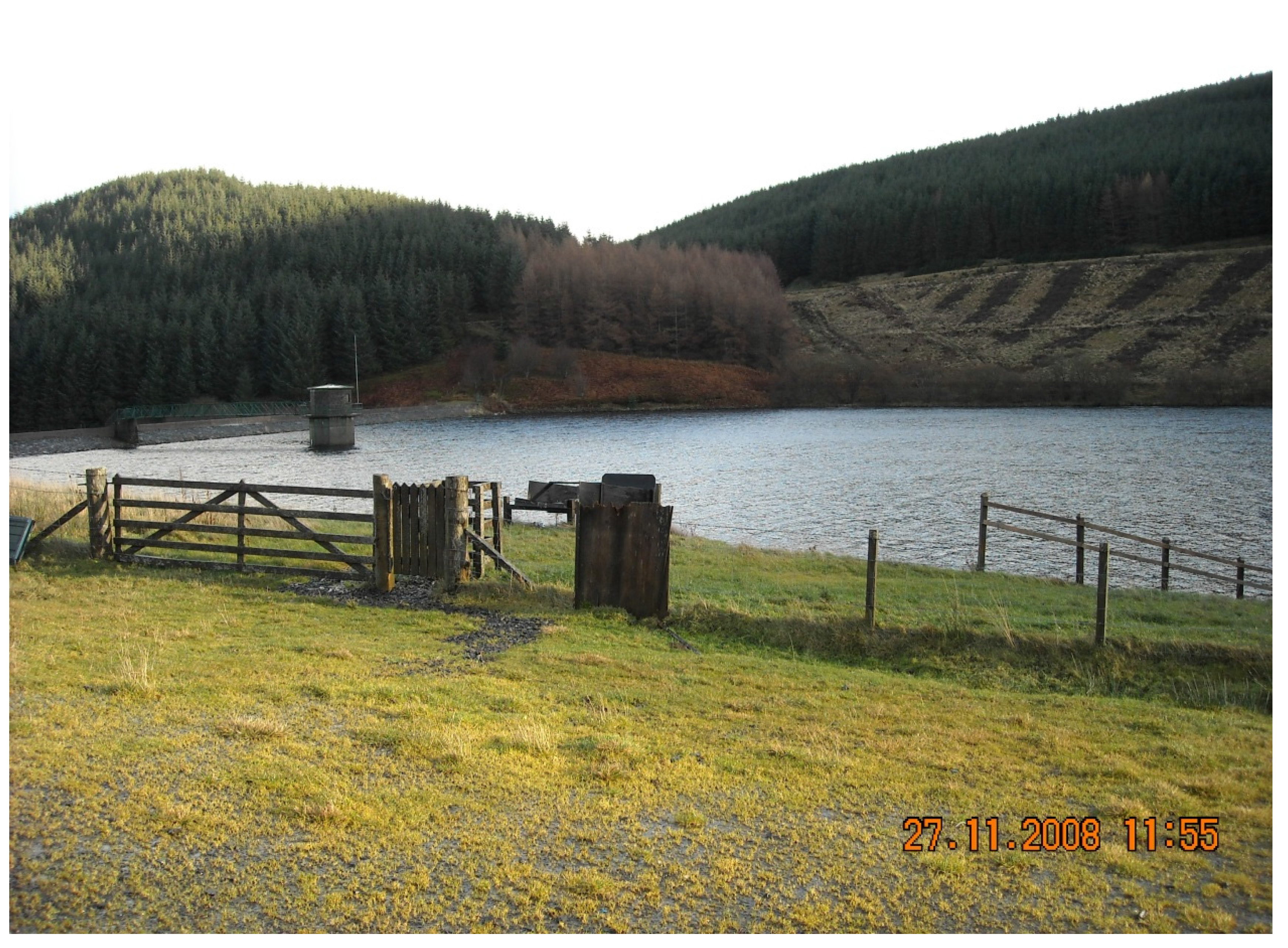
Take Glensherup Reservoir (56°7'48'' N, 3°24'3'' W, Figure 5) as a case study. It is located on a tributary of the River Devon, operated by Scottish Water. The reservoir was built in 1883, and has a catchment size of 5.5 km². It provides drinking water to the city Glendevon, which indicates that the water body belongs to SFRB type 2. Furthermore, it allows the community to undertake recreational activities such as fishing and walking, which shows that the reservoir also belongs to SFRB type 5. The traditional classifier SVM predicted the reservoir to be SFRB type 2. After integrating uncertainty, the reservoir was predicted to belong to SFRB types 2 and 5 (Table 2).

Table 4. Classification results of sustainable flood retention basins by using a multi-instance multi-label learning algorithm-support vector machine (MIML-SVM) and SVM. (mean ± standard deviation).

Algorithm	K	Evaluation Criteria
		Ham.-L. ml	Ran.-Loss	One-Error	Coverage	Avg. Pre.
MIML-SVM	10	0.094 ± 0.029	0.051 ± 0.027	0.097 ± 0.057	0.768 ± 0.057	0.935 ± 0.031
	30	0.092 ± 0.022	0.049 ± 0.020	0.082 ± 0.060	0.761 ± 0.149	0.935 ± 0.029
	50	0.091 ± 0.018	0.049 ± 0.018	0.087 ± 0.033	0.750 ± 0.120	0.935 ± 0.020
	70	0.093 ± 0.028	0.049 ± 0.024	0.087 ± 0.058	0.758 ± 0.191	0.934 ± 0.029
	100	0.089 ± 0.023	0.048 ± 0.015	0.087 ± 0.048	0.753 ± 0.119	0.936 ± 0.024
	Mean	0.092 ± 0.024	0.049 ± 0.021	0.088 ± 0.051	0.758 ± 0.157	0.935 ± 0.027
SVM		Accuracy	Precision	Recall	F1
		0.847 ± 0.023	0.842 ± 0.025	0.847 ± 0.013	0.843 ± 0.024

Notes: Ham.-L.^ml: Hamming-loss; Ran.-Loss: Ranking-Loss; Avg. Pre.: Average Precision.

Table 4. Classification results of sustainable flood retention basins by using a multi-instance multi-label learning algorithm-support vector machine (MIML-SVM) and SVM. (mean ± standard deviation).

Algorithm	K	Evaluation Criteria
		Ham.-L. ml	Ran.-Loss	One-Error	Coverage	Avg. Pre.
MIML-SVM	10	0.094 ± 0.029	0.051 ± 0.027	0.097 ± 0.057	0.768 ± 0.057	0.935 ± 0.031
	30	0.092 ± 0.022	0.049 ± 0.020	0.082 ± 0.060	0.761 ± 0.149	0.935 ± 0.029
	50	0.091 ± 0.018	0.049 ± 0.018	0.087 ± 0.033	0.750 ± 0.120	0.935 ± 0.020
	70	0.093 ± 0.028	0.049 ± 0.024	0.087 ± 0.058	0.758 ± 0.191	0.934 ± 0.029
	100	0.089 ± 0.023	0.048 ± 0.015	0.087 ± 0.048	0.753 ± 0.119	0.936 ± 0.024
	Mean	0.092 ± 0.024	0.049 ± 0.021	0.088 ± 0.051	0.758 ± 0.157	0.935 ± 0.027
SVM		Accuracy	Precision	Recall	F1
		0.847 ± 0.023	0.842 ± 0.025	0.847 ± 0.013	0.843 ± 0.024

Notes: Ham.-L.^ml: Hamming-loss; Ran.-Loss: Ranking-Loss; Avg. Pre.: Average Precision.

Figure 5. Glensherup Reservoir (56°7'48'' N, 3°24'3'' W) is a typical example of a sustainable flood retention basin (SFRB) belonging to SFRB types 2 and 5.

Figure 5. Glensherup Reservoir (56°7'48'' N, 3°24'3'' W) is a typical example of a sustainable flood retention basin (SFRB) belonging to SFRB types 2 and 5.

Type 5 is closer to the reality, recognizing the dual function of the reservoir: drinking water provision and multiple recreation functions. This has implications on policy. For example, Scottish Water has the obligation to manage the reservoir in terms of health and safety, taking responsibility for visitors by creating safe paths and parking spaces. On the other hand, visitors might not be allowed to swim in parts of the reservoir, particular if the water level is low.

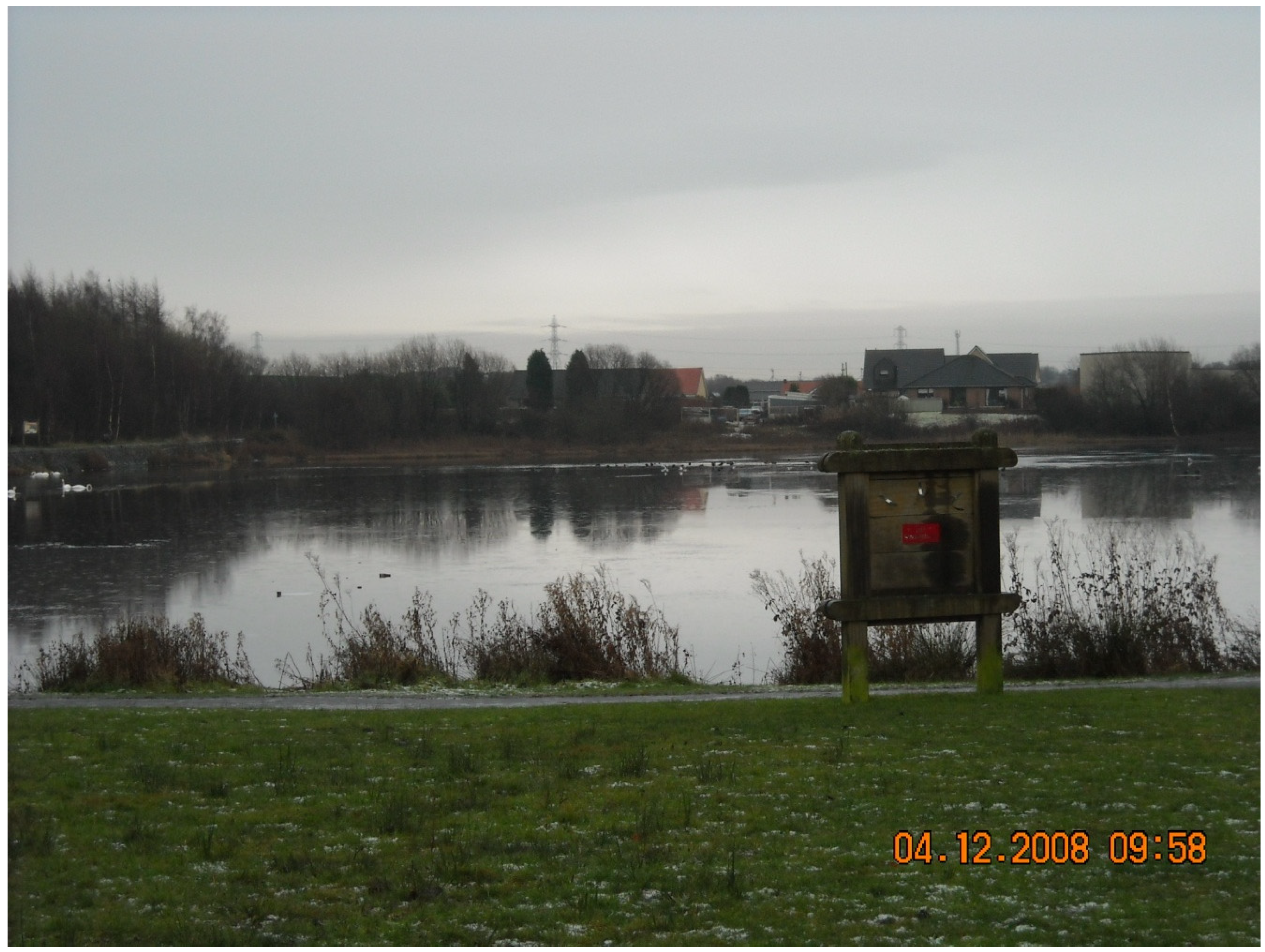
Take Garnqueen Loch (55°53'24'' N, 4°3'5'' W, Figure 6) located in North Lanarkshire as another example. The loch (Scottish for “lake”) is a natural water body without a man-made dam and supports a healthy variety of aquatic plants and many other reed grasses. Furthermore, various birdlife (e.g., mute swan, moorhen and tufted duck) and fish life (e.g., perch and roach) also live on and under the surface of the loch, respectively. The loch is located in the Glenboig Village Park and has been developed for recreational activities and drainage of the surrounding area. Based on the above prior knowledge, experts judge the loch to fall under SFRB types 3, 5 and 6. The original estimations of some representative variables for Garnqueen Loch are recorded as follows (variable data, confidence level): engineered (10%, 90%); dam height (0 m, 100%), drainage (1.2 cm/day, 75%), vegetation cover (20%, 85%) and urban catchment proportion (40%, 80%). Without considering the uncertainty issue, the loch was predicted to belong to SFRB type 5 by the SVM classifier. After the input uncertainty was modeled, the proposed new classification scheme predicted it to be SFRB types 3, 5 and 6 (Table 2), which is consistent with expert judgment.

Figure 6. Garnqueen Loch (55°53'24'' N, 4°3'5'' W) is a typical example of a sustainable flood retention basin (SFRB) belonging to SFRB types 3, 5 and 6.

Figure 6. Garnqueen Loch (55°53'24'' N, 4°3'5'' W) is a typical example of a sustainable flood retention basin (SFRB) belonging to SFRB types 3, 5 and 6.

The new classification methodology recognizes the multi-functionality of the loch not just for recreational purposes but also for sustainable drainage and nature conservation. It follows that the municipality has the obligation to manage the loch for multiple stakeholders. In practice, this means managing potentially conflicting interests fairly and appropriately. For example, recreational activities might have to be limited during the bird nesting season. On the other hand, wildlife has to cope with visitors during the summer.

The improved classification performance is mainly due to the uncertainty model as it is effective in encoding the intrinsic properties of water bodies into an intuitive probability function. Modeling the uncertainty with a set of instances using Monte Carlo sampling means one instance among them should be closer to the true values, and it will be automatically selected and educated by multi-instance multi-label learning. Therefore, it is evident that input uncertainty and output uncertainty are closely correlated, and performance in predicting multiple functions of SFRBs highly depends on whether someone can effectively model the input data uncertainty.

The function of a water body such as an SFRB may change over time due to a changing environment. For instance, one basin might have initially been designed for hydropower generation (SFRB type 1) in a sub-urban area. However, after several decades, urban expansion and population growth in the downstream area may demand much more drinking water. Thereby, the SFRB previously used for hydropower generation may be requested to perform an additional new function, i.e., drinking water supply. It follows that the basin now belongs to SFRB types 1 and 2. Except for human activities, climate change can also result in SFRB type change via precipitation-runoff pattern alterations. Therefore, to adaptively manage water resources, the function assessment of SFRBs needs to be updated, allowing for multiple functions (types).

In this study, to characterize SFRBs, 40 easy, accessible variables have been collected to support a rapid and efficient classification model. However, this general data-driven model is not restricted to a fixed number of input variables, and more variables can be investigated such as ecological and sustainability parameters like habitats or rare species, adapting to the requirements of practical problems.

Moreover, the framework might also be extended and applicable to other related environmental studies, considering that the authors provide a general model for classification under uncertainty based on multi-instance multi-label learning. The proposed tool should be of particular interest to policy makers and implementers, because it provides an unbiased framework for decision-makers balancing the interests of different stakeholders such as the water industry, municipalities, agriculture, forestry, fisheries and the public.

4. Conclusions and Recommendations

To assess the functions of a large number of SFRBs in a relatively short time period with a limited number of experts is a challenge for water resources managers and planners. To rapidly assess and distinguish the multiple functions of sustainable flood retention basins (SFRBs) under uncertainty, the authors have developed a data-driven framework based on multi-instance multi-label learning scheme. A Gaussian-based model with Monte Carlo sampling was proposed to reflect the intrinsic uncertainty of the properties of SFRBs. Multi-instance multi-label learning was further introduced to predict the multiple potential functions of basins.

The study shows that by taking uncertainty into account, the prediction of MIML-SVM achieves an average precision as high as 93.5%, outperforming that of the traditional SVM algorithm (84.7%). The more accurate prediction is due to the superior characterization of water bodies with the proposed uncertainty model, which investigates the input and output uncertainties simultaneously. The proposed framework will help water resources managers and planners to better understand the diverse potential functions of SFRBs, which has been demonstrated by two case study examples.

Case studies demonstrated that the proposed framework provides an intuitive way to model uncertain data. For example, the classification of SFRBs is more accurate after taking confidence levels into account. It thus helps to better study the diverse potential functions of SFRBs based on pattern classification.

The major knowledge contributions from this study are as follows: (a) Taking uncertainty into account, the proposed model provides a rapid and effective tool to predict the multiple potential functions of SFRBs in a comprehensive way; (b) The input and output uncertainty are investigated simultaneously, and the multi-instance multi-label learning scheme is naturally introduced to handle a case study problem; and (c) The proposed framework not only complements the study of SFRBs but also has the potential to be applicable to many other water and environmental studies, as this novel and timely approach provides a generic method to handle input and output uncertainty simultaneously.

In the future, the authors will further integrate more variables to characterize SFRBs, and consider the distinct roles of variables for classification via some weighting schemes. The team also recommends that the Environment Agency’s current project entitled “Design, Operation and Adaptation of Flood Storage Reservoirs” should consider the SFRB concept and its associated classification methods when updating the existing national guidance for flood storage reservoirs in 2015 and 2016.