Review

Assessment of Agricultural Best Management Practices Using Models: Current Issues and Future Perspectives

State Key Laboratory of Water Environment, School of Environment, Beijing Normal University, Beijing 100875, China
*
Author to whom correspondence should be addressed.
Water 2015, 7(3), 1088-1108; https://doi.org/10.3390/w7031088
Submission received: 15 December 2014 / Revised: 16 February 2015 / Accepted: 24 February 2015 / Published: 12 March 2015
(This article belongs to the Special Issue Water Quality Control and Management)

Abstract

:
Best management practices (BMPs) are the most effective and practicable means to control nonpoint source (NPS) pollution at desired levels. Models are valuable tools to assess their effectiveness. Watershed managers need to choose appropriate and effective modelling methods for a given set of conditions. This paper considered state-of-the-art modelling strategies for the assessment of agricultural BMPs. Typical watershed models and specific models were analyzed in detail. Further improvements, including simplified tools, model integration, and incorporation of climate change and uncertainty analysis were also explored. This paper indicated that modelling methods are strictly scale dependent, both spatially and temporally. Despite current achievements, there is still room for future research, such as broadening the range of the pollutants considered, introducing more local BMPs, improving the representation of the functionality of BMPs, and gathering monitoring date for validation of modelled results. There is also a trend towards agricultural decision support systems (DSSs) for assessing agricultural BMPs, in which models of different scales are seamlessly integrated to bridge the scale and data gaps. This review will assist readers in model selection and development, especially those readers concerned about NPS pollution and water quality control.

1. Introduction

In the last few decades, nonpoint source (NPS) pollution from agricultural lands has caused major water quality degradation and threatened the safety of water resources worldwide. One of the most crucial issues for protecting water quality is how to effectively control NPS pollution [1,2]. Best management practices (BMPs) are routinely used, yet there has been much concern regarding the efficiency of BMPs in reducing NPS loads [3]. Assessment of BMPs, which has become a thriving area of research, can ensure the most effective use of funding for watershed management and can avoid the implementation of unreasonable practices. Models, which represent the optimal assimilation of physical, chemical, and biological watershed processes, have been proposed to evaluate the impact of BMPs on NPS pollution. Currently, modelling is integrated as a necessary step in watershed management, such as through the Total Maximum Daily Load (TMDL) in the United States and the Water Framework Directive in Europe [4,5].
Models for assessing agricultural BMPs can be divided into various types based on their complexity and scales of application. Watershed models evaluate the hydrologic and water quality response to multiple BMPs at varying scopes and locations. Their application has also been expanded to the basin and regional scales [6]. For example, by incorporating Geographic Information System (GIS) techniques, cropland conversion to forest/grassland as an effective BMP can be easily evaluated by watershed models. In a study of the upper reaches of the Yangtze River by Ouyang et al. [7], the land use scenario assumed that croplands were converted to forests. The results from a watershed model revealed that when agricultural lands with slopes greater than 7.5° were converted to forests, the organic nitrogen and organic phosphorus decreased by 42.1% and 62.7%, respectively. In contrast, several structural BMPs are commonly implemented at the field scale at which the utility of watershed models is limited [8]. For these widely used BMPs (e.g., filter strips, riparian buffers, and detention ponds), specific assessment models have been developed [9,10]. Site-specific conditions and dimensions of agricultural BMPs are incorporated into these specific models, which are often beyond the capacity of most watershed models.
Watershed models and specific models are both effective tools for agricultural BMP assessment, but they are not always used appropriately. There is still room for model improvements to facilitate the assessment process. In general, the selection of an appropriate approach will greatly influence decision making regarding watershed plans and regulations. There is a large body of published literature on the assessment of agricultural BMPs using models, yet a systematic review conducive to model selection and development is lacking. This review aims to fill that void. Our objectives are to (i) critically review state-of-the-art, model-based assessment methods for agricultural BMPs; (ii) compare commonly used watershed models and specific models based on their strengths and limitations; (iii) discuss model improvements to facilitate the assessment of agricultural BMPs; and (iv) propose several implications for future trends.

2. Commonly Used Models for Assessing Agricultural Best Management Practices (BMPs)

Based on a thorough literature evaluation, we identified 17 models which have been used for assessment of agricultural BMPs. They are Soil and Water Assessment Tool (SWAT) [11], Agricultural Nonpoint Source (AGNPS) [12], Annualized Agricultural Nonpoint Source (AnnAGNPS) [13], Hydrological Simulation Program-FORTRAN (HSPF) [14], Vegetative Filter Strip Model (VFSMOD) [15], Riparian Ecosystem Management Model (REMM) [16], Agricultural Policy/Environmental eXtender (APEX) [17], Groundwater Leaching Effects of Agricultural Management Systems (GLEAMS) [18], Generalized Watershed Loading Functions (GWLF) [19], Erosion-Productivity Impact Calculator (EPIC) [20], Pollution Load (PLOAD) [21], Dynamic Watershed Simulation Model (DWSM) [22], Areal Nonpoint Source Watershed Environment Response Simulation (ANSWERS) [23], Water Erosion Prediction Project (WEPP) [24], Universal Soil Loss Equation (USLE) [25], MIKE SHE/MIKE 11 coupling model [26], and WETLAND [27]. The first six models are chosen as the most representative models for this review. The main reason is that they are more frequently used in comparison with other models, which can be recognized by the extent of publication in English. Our selection also assures the most common BMPs can be evaluated by the selected models, by which typical methods for the assessment cover scales (field to watershed) and scopes (structural and non-structural measures, sediment, nutrient, and pesticide processes) for comparative purpose. Other models are excluded from this review mainly because of the following considerations: (i) Similar algorithms and structures in models which however have limited application; (ii) Inability to interpret nutrient process; and (iii) Lack of ongoing development for the assessment of BMPs. Following these criteria, we then selected six models. The first four models were further categorized as watershed models and the other two models are specific models.

2.1. Watershed Models

The SWAT, AGNPS, AnnAGNPS, and HSPF are four watershed models selected for this review. Table 1 provides a listing from the existing literature of their use for assessment of agricultural BMPs. The characteristics, including spatial representation, temporal resolution, and watershed process descriptions under BMPs conditions, are briefly summarized in Table 2.
Table 1. The summary of the studies on agricultural BMPs’ assessment using watershed models.
BMPStudy AreaModelPollutants of ConcernRef.
Tillage management; Contour farming; Grazing management, Native grass; Residue management; TerraceTuttle Creek Lake watershed, USA, 6,158 km2SWATSediment and nutrient[28]
Contour farming; Residue management; Strip cropping; Native grass; Terrace; Recharge structureSaginaw River watershed, USA, 15,263 km2SWATSediment and nutrient[29]
Cover crop; Filter strip; Residue managementRiver Raisin watershed, USA, 268,100 haSWATSediment[30]
Crop rotation; Terrace; Sediment basinPipiripau River basin, Brazil, 235 km2SWATSediment[31]
Nutrient management; Grass waterway; Grade stabilization structure; Tillage management; Residue managementEagle Creek Watershed, USA, 248.1 km2SWATSediment, nutrient, and pesticide[32]
Nutrient management; Tillage management; Filter stripWider Arachtos catchment, Greece, 2,000 km2SWATNutrient[33]
Pasture management; Poultry management; Buffer zoneLincoln Lake watershed, USA, 32 km2SWATNutrient[34]
Residue management; Filter strip; Pond; Grassed waterway.Orestimba Creek watershed, USA, 563 km2SWATPesticide[35]
Detention pondFeitsui Reservoir watershed, Taiwan, China, 303 km2HSPFSediment and nutrient[36]
Filter stripSouth Farm Research Park, USA, 20.17 acresHSPFSediment and nutrient[37]
Constructed wetland; Detention pondHan River Basin, Korea, 20,271 km2HSPFNutrient and BOD5[38]
Contour farming; TerraceMiddle Seydi Suyu watershed, Turkey, 414 km2HSPFSediment[39]
Cropland conversion; Tillage management; Sedimentation basinsNorth Reelfoot Creek watershed, USA, 146 km2HSPFSediment[40]
Cropland conversion; Contour farming; Nutrient management; Multi-pond systemWuchuan watershed, China, 188 haAGNPSSediment and nutrient[41]
Terrace; Grass waterway; Filter stripPosan Reservoir, Singapore, Not mentionedAGNPSSediment and nutrient[42]
Tillage management; Strip cropping; Livestock stream access control; Terrace; Grass waterway; Filter stripOwl Run watershed, USA, 1,153 haAGNPSSediment and nutrient[43]
Cropland conversion; Contour farming; Nutrient management; Filter stripZhangxi River watershed, China, 8,970 haAnnAGNPSSediment, nutrient, and TOC[44]
Nutrient management; Tillage management; Livestock stream access controlSouth Nation watershed, USA, 3,900 km2AnnAGNPSNutrient and TOC[45]
Detention pondA hypothetical watershed, 1,172 haAnnAGNPSSediment[46]
Cover crop; Tillage management; Filter strip; Cropland conversion; PondDeep Hollow Lake watershed, USA, 82 haAnnAGNPSSediment[47]
Table 2. Brief description of watershed models with respect to BMPs’ assessment.
ModelsTemporal ResolutionSpatial RepresentationOverland Flow RoutingOverland Sediment RoutingChannel ProcessesDeveloper
SWATContinuous; Daily or sub-daily time steps.Sub-basins or further hydrologic response units defined by soil and land use/land cover.SCS-CN a method for infiltration and peak flow rate by modified Rational formula.MUSLE b represented by runoff volume, peak flow rate, and USLE c factors.Channel degradation and sediment deposition process including channel-specific factors.USDA d
AGNPSStorm-event; One storm duration as a time step.Cells of equal size with channels included.SCS-CN method for infiltration, and flow peak using a similar method with SWAT.USLE for soil erosion and sediment routing through cells with n, USLE factors to be concerned with.Included in overland cells.USDA e
AnnAGNPSContinuous; daily or sub-daily time steps.Cells with homogeneous soil and land use.SCS-CN method for infiltration and TR-55 f method for peak flow.RUSLE g to generate soil erosion daily or user-defined runoff event.Channel degradation and sediment deposition with Modified Einstein equation and Bagnold equation.USDA
HSPFContinuous; variable constant steps (from 1 min up to 1 day).Pervious and impervious land areas, stream; hydrologic response units.Philip’s equation for infiltration.Rainfall splash and wash off of detached sediment calculated by an experimental non-liner equation.Non-cohesive and cohesive sediment transport.USGS h and USEPA i
Nots: a Soil Conservation Service curve number; b Modified Universal Soil Loss Equation; c Universal Soil Loss Equation; d United States Department of Agriculture; f Technical Release-55; g Revised Universal Soil Loss Equation; h United States Geological Survey; i United States Environmental Protection Agency.

2.1.1. Spatial Scale and Watershed Representation

The way a watershed is discretized determines the basic computational units in which certain types of BMPs are simulated. The appropriate spatial scale at which models operate effectively under BMP conditions can be defined based on a comparison of watershed segmentation methods. On basis of a Digit Elevation Model (DEM), the SWAT model discretizes a watershed into sub-watersheds and stream reaches based on surface topography. A sub-watershed is further divided into hydrologic response units (HRUs). A typical HRU is comprised of a homogeneous land use, soil attribute, and slope. Runoff, sediment, and contaminant loadings from each HRU are calculated separately and then summed together at the sub-watershed level and then routed through reach segments and to the basin outlets [48]. Parameters, or inputs related to pollutant removal mechanisms, are lumped in sub-watersheds, HRUs, and reaches, which enables SWAT to evaluate BMPs at the watershed and sub-watershed scales. HRUs may represent the field-level conditions for BMPs, but there is a distinct disconnect between the hydrologic scale of HRUs and the actual fields at which these BMPs are implemented.
The AGNPS model divides a watershed into cells of equal size which are the basic spatial units for simulating BMPs [49]. As an expanded version of AGNPS, AnnAGNPS enhances the previously described discretization method by delineating cells, reaches, and impoundments based on topographic homogeneity similar to the SWAT model [50]. Cells are almost identical to sub-watersheds in SWAT but have no subdivisions, such as HRUs. The HSPF model, as an inherent component of Better Assessment Science Integrating Point and Nonpoint Sources (BASINS) [51], can also divide a watershed into sub-watersheds and reaches. Simulations are conducted within homogeneous land segments called HRUs. The HSPF model can be applied at different scales (ranging from a few hectares up to 128,000 km2) [52] due to its flexible, user-defined definition of HRUs. Moreover, a HRU in the HSPF model is connected to an adjacent HRU or a reach. Runoff and water quality constituents resulting from agricultural BMPs leave each HRU and route laterally to down-slope land segments or streams. Therefore, the model can simulate the relationship between successive BMPs at smaller scales, which is not possible in the SWAT model [52].
Actually, neither square units (cells in AGNPS) nor irregularly shaped units (cells in AnnAGNPS and HRUs in SWAT and HSPF) can exactly represent the actual positions of BMPs. Ghebremichael et al. [53] suggested that HRUs in the SWAT model may be manually defined based on the spatial field boundary. Alternatively, the topographic, soil, and land use thresholds may be set to 0% to capture the detailed watershed processes. HRUs may be assigned to their original locations while the HRU-outputs may be transformed to field-level results [54]. Adjustments to the parameters and inputs related to BMP characteristics under pre-BMP and post-BMP periods are common principles for representing agricultural BMPs for field scale assessment. In addition, the watershed segmentation strategies discussed above may be inappropriate for BMPs located in special hydrogeological conditions. For example, riparian buffers receive pollutants from upland drainage areas and transfer them to adjacent streams. This interaction mechanism is important for BMPs functioning though is oversimplified in the watershed models.

2.1.2. Temporal Scale and Resolution

Certain BMPs (e.g., sediment basins and vegetative filter strips) should be designed for single events during sudden storm events, which is the current requirement of TMDL [5]. Rainfall intensity, duration, and intra-event variability of flow and pollutants are required to assess their ability to model storm event. So, the application of watershed models for assessing BMPs is also limited by temporal resolution which ranges from annual to sub-hourly averages. The SWAT model usually operates continuously at a daily time step [29], which ensures that the long-term impacts of BMPs can be quantified. Sub-daily calculations of runoff, erosion, and sediment transport are also available in new version of SWAT by sub-daily rainfall input and Green & Ampt method [55], though few attempts have obtained a higher temporal resolution. In a recent study by Maharjan et al. [56], hourly runoff prediction at a small watershed was quite acceptable with both coefficient of determination and Nash and Sutcliffe Efficiency greater than 0.8 during calibration and validation. A sub-daily erosion and sediment transport algorithm was also incorporated into SWAT model, which is found adequate for simulating detention-based BMPs (e.g., sediment basins and ponds) [10]. Further research should extend to NPS pollution with SWAT model at the sub-daily pattern.
The HSPF model can simulate watershed processes at event-step to long-term steps [57], but storage-based or nonlinear flow routing equations in the HSPF model are insufficient for representing intense or even extreme storm events [58]. The AGNPS model can simulate the change in water quality after a storm event. The single-event pattern cannot perceive the long-term features of several BMPs. The hydrographs during an individual event are also not included. The AnnAGNPS model significantly improved many of the features of its predecessor. The most notable modification is that the AnnAGNPS model can also be operated on a daily and sub-daily step, which facilitates the generation of many non-structural BMP scenarios [59]. Overall, the advantage of most of the reviewed watershed models lies in their capacity to simulate the long-term impacts of proposed BMPs, which is inappropriate if we focus on the design of storm-based agricultural BMPs.

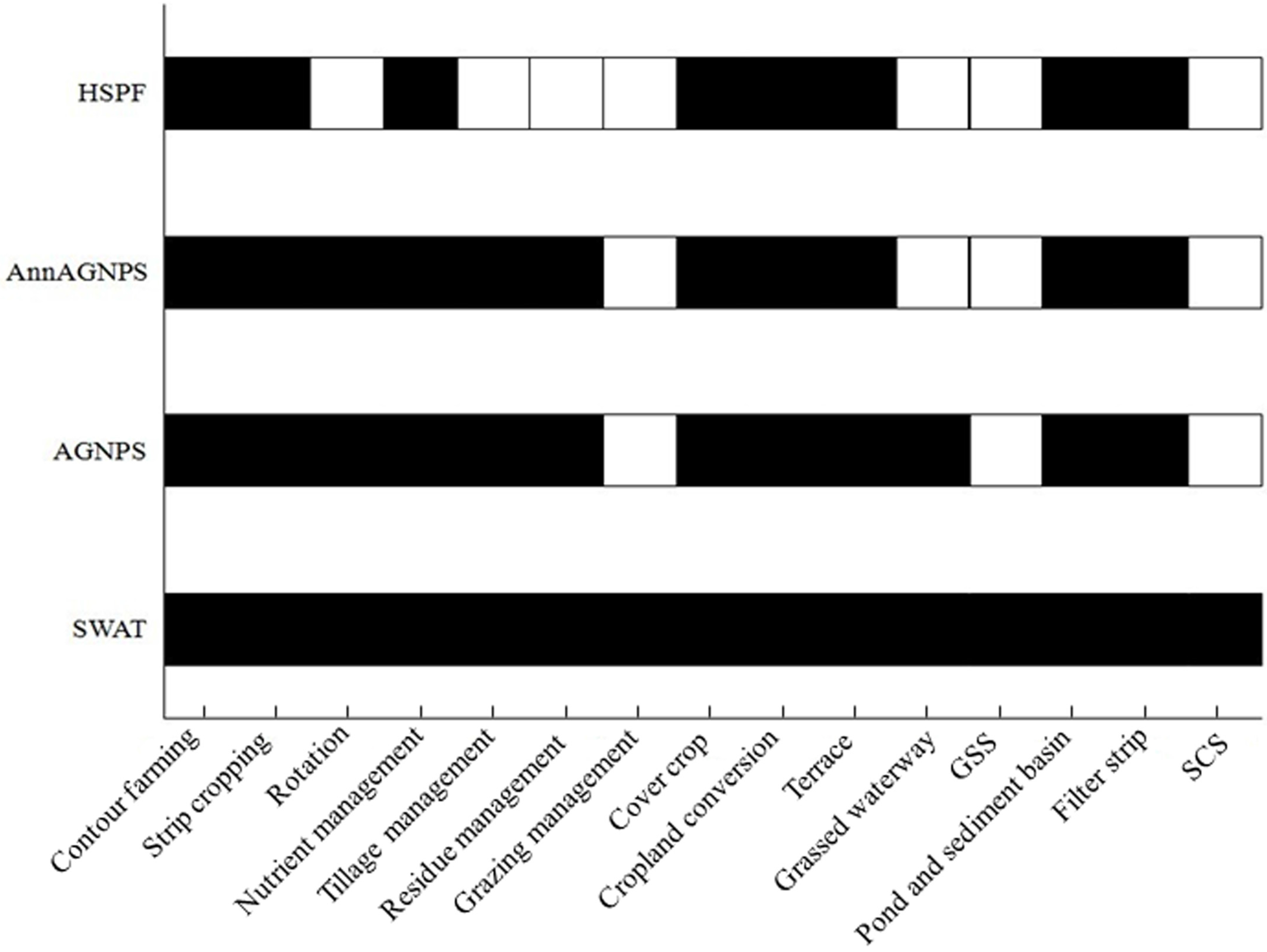
2.1.3. Representation of BMPs

The common principle of BMPs representation is to depict the change in watershed processes and the response of water quality under or without BMPs by changing model inputs or parameter values. In this sense, watershed models are generally the conceptualization of the way in which the BMPs are functioning at the watershed scale. The types of agricultural BMPs that can be assessed by different watershed models are shown in Figure 1. The cause of the discrepancy is mostly due to model structures and algorithms.
Figure 1. Typical agricultural BMPs which can be assessed by each watershed model. (Black squares indicates that the model can address those BMPs and white squares indicates the opposite. GSS: Grade stabilization structure. SCS: Stream channel stabilization).
Water 07 01088 g001
Agricultural BMPs focus on source loading reduction and pollution transport control. Source loading reduction measures may relate to cropland conversion, nutrient (manure and fertilizer) management, integrated pesticide management, poultry management, and grazing management. Croplands are considered as the major source of NPS pollution, the reduction of which has been found to occur in response to the shifts of croplands to less erosive use [7,60]. One approach for representing cropland conversion by watershed models is to use GIS techniques to adjust land use maps. Alternatively, SWAT model introduce a land use change (LUC) module, which allows manually adjusting fractional coverage of land use types in each HRUs [61]. Pai and Saraswat [62] further developed an automated tool to ingest multiple land use information and activate the LUC module. For other BMPs addressing source loading reduction, the SWAT model allows information about these measures to be modified by scheduling the amount, timing and period of agricultural activities [21]. The management file, HRU file, and database files contain the input information, which can be adjusted [63]. By contrast, the AGNPS and AnnAGNPS models have no specific options for agricultural management practices, but they use BMP-responsive inputs (fertilization level, the availability factor, and rate of fertilizer applied) to represent nutrient management [43]. However, there are no documented studies reporting the application of AGNPS and AnnAGNPS models in the field for evaluating pesticide control or poultry and grazing management (see Figure 1). The main reason lies in their rough sketch of farming practices.
For transport control BMPs, physically based algorithms in watershed models can be used by altering the values of parameters sensitive to the functioning of the BMPs. The removal mechanism of a typical BMP involves watershed processes, including interception, infiltration, overland flow, interflow, evapotranspiration, sheet and rill erosion, contaminant routing, and within-channel processes [64]. The key input parameters and processes in watershed models (SWAT, AGNPS/AnnAGNPS) used to represent agricultural BMPs for pollution transport control are summarized in Table 3.
Table 3. Key parameters and processes of watershed models (SWAT, AGNPS/AnnAGNPS) for representing BMPs.
BMPModelSurface RunoffOverland Sediment RoutingChannel ProcessSpecific Module
TerraceSWATCNP factor, LS factor
AGNPS/AnnAGNPSCNP factor, LS factor
Strip croppingSWATCN, nP factor, C factor
AGNPS/AnnAGNPSCN, nP factor, C factor
Contour farmingSWATCNP factor
AGNPS/AnnAGNPSCNP factor
Residue managementSWATCN, nC factor
AGNPS/AnnAGNPSCN, nC factor
Tillage managementSWATCN, EFFMIX a, DEPTIL bCN, EFFMIX, DEPTIL
AGNPS/AnnAGNPSCN, nC factor
Filter stripSWAT VFS routine
AGNPS/AnnAGNPSn, land use
Grassed waterwaySWAT CH_depth, CH_width, CH_COV, CH_n
AGNPS/AnnAGNPS CH_n, zero gully sources
Grade stabilization structureSWAT CH_SLOP, CH_EROD
Stream channel stabilizationSWAT CH_EROD, CH_n
Sediment basins and detention pondSWAT Impoundment
AGNPS/AnnAGNPS Impoundment
Notes: a EFFMIX: The mixing efficiency of a tillage options; b EFFTIL: Depth of mixing caused by tillage options.
The SWAT, AGNPS and AnnAGNPS models are agriculture-oriented and employ rather similar equations to quantify the impact of agricultural BMPs. In upland areas, overland flow routings in SWAT, AGNPS, and AnnAGNPS models are related to curve number (CN) and Manning’s roughness coefficient (n). Adjustments to CN and n values represent BMPs that decrease surface runoff by increasing infiltration (e.g., contour farming, terracing, and strip cropping) and decrease flow rate by intercepting runoff (e.g., residue management and strip cropping), respectively. The simulation of the impact of BMPs on sheet and rill erosion in overland areas is also quite similar in these three models. The Universal Soil Loss Equation (USLE) and its associated forms, the Revised Universal Soil Loss Equation (RUSLE) and the Modified Universal Soil Loss Equation (MUSLE), are respectively incorporated in the AGNPS, AnnAGNPS and SWAT models. The RUSLE and USLE have the same formula as Equation (1) while MUSLE is represented by Equation (2):
A = R · K · L S · C · P
s e d = 11.8 · ( Q s u r f · q p e a k · a r e a h r u ) 0.56 · K · C · P · L S · C F R G
where A is the average annual soil loss, and sed is the sediment yield on a given day. R is the rainfall erosivity factor; K is the soil erodibility factor; Qsurf is the surface runoff volume; qpeak is the peak runoff rate; and areahru is the area of the HRU. The common parameters in the above equations include the cover and management (C) factor, the support practice (P) factor, and the topographic (LS) factor. Each of these factors can be adjusted to represent the adoption of agricultural BMPs (e.g., terracing, contour farming, strip cropping and residue management).
As for the channel network, the Bagnold or Einstein equation for the calculation of sediment routing within the SWAT, AGNPS and AnnAGNPS models define Manning’s roughness coefficient (CH_n) to calculate channel flow capacity which influences sediment deposition and the relevant pollution loadings [58]. So CH_n can be altered in watershed models to represent the impact of many channel BMPs (e.g., grassed waterways, lined waterways, and stream stabilization). Specifically, SWAT introduces two BMP-responsive parameters: The channel erodibility factor (CH_EROD), which is a function of the properties of the bed or bank material, and the channel cover factor (CH_COV), which is defined by vegetative cover [63]. These two parameters as well as channel geometric parameters (CH_width, CH_depth and CH_SLOP) enhance the evaluation ability of the SWAT model to assess the impact of BMPs on the channel network.
As a structural BMP, vegetative filter strips (VFSs) are widely used to mitigate sediment and nutrient levels in runoff before it reaches water bodies. Their effectiveness has been assessed by the SWAT model in many studies [30,35]. However, in the previous versions of the SWAT model (before SWAT 2009), the same efficiency was assigned to sediments and all nutrient forms, which is problematic according to field investigations. The effects of flow concentration that are apparent at various scales were also neglected [8]. The new routine (developed in SWAT 2009) employs different filtering efficiencies for all forms of sediments and nutrients. A VFS is divided into two sections to consider the concentrated flow: Section one where 90% of the VFS receives the least flow and section two where the remaining 10% of the area receives the major runoff (25%–75%). The drainage area to VFS section one (DAFSratio1) and drainage area to VFS section two (DAFSratio2) are calculated using the Equations (3) and (4):
D A F S r a t i o 1 = D A F S r a t i o ( 1 D F c o n ) / 0.9
D A F S r a t i o 2 = D A F S r a t i o ( 1 C F f r a c ) / 0.1
Three additional parameters can be altered to describe the new structures of the VFSs in the SWAT model: The drainage area to VFS area ratio (DAFSratio), the fraction of the field drained by the most heavily loaded 10% of the VFS (DFcon), and the fraction of the flow through the most heavily loaded 10% of the VFS that is fully channelized (CFfrac) [8]. In contrast, AGNPS and AnnAGNPS models have no specific routines to assess VFSs. The most common way to represent VFSs is to change the current land use type to grasslands or increase the value of n [43]. The SWAT and AnnAGNPS models can also treat BMPs like sediment basins and detention ponds as impoundments, which can be simulated in their specific modules. PND_K (bottom permeability coefficient), PND_FR (fraction of sub-watershed area draining to the pond), PND_PSA (surface area of ponds) and PND_PVOL (volume of the ponds) in the SWAT model can be adjusted for sediment loss calculation [65]. For the AnnAGNPS model, sediment accumulation and resuspension processes were added to generate an accurate representation of sediment basins and detention ponds [46]. Decisive inputs, such as the detention time for a specific storm and a pond’s geometric parameters (surface area, depth), can be modified in the context of watershed-scale modelling.
The HSPF model has a unique module called BMPRAC (Best Management Practice Evaluation) to facilitate the assessment of many structural BMPs [14]. In the BMPRAC, modellers can use recommended removal fractions pertaining to an assumed BMP [38]. However, these removal fractions are based on documented studies conducted in diverse conditions. The assignment of user-defined values to the effectiveness of BMPs at a site-specific area may lead to crude or even indeterminate results. Another module of HSPF, called SPEC-ACTIONS, allows detailed inputs related to management activities, including ploughing, planting, harvesting, and pesticide and nutrient application [66]. Thus, this module is useful for representing agricultural improved management practices.

2.2. Specific Models

Watershed models are more often used for assessment at the watershed and sub-watershed scales. However, some BMPs, especially structural BMPs, are implemented at the field level where the response of water quality to these BMPs deserves more attention [67]. VFSs and riparian buffers are widely used structural BMPs, and specific models have been developed for the assessment of their trapping mechanisms. In this section, two specific models, VFSMOD and REMM, are discussed in detail.
VFSMOD is an event-based model that routes the incoming hydrograph and sediment graph to simulate outflow, infiltration, and sediment trapping under field conditions [68]. It uses many physical parameters to represent site-specific characteristics, including vegetation type, geometric shape (length and width), land slope, and soil properties. It should be noted that nutrient and pesticide processes are excluded from the original version of VFSMOD. However, Kuo and Muñoz-Carpena [69] and Sabbagh et al. [70] coupled VFSMOD to empirical trapping efficiency equations for phosphorus and pesticides, respectively. The enhanced model was also combined with a graphical user interface and other tools to develop a vegetative filter strip modelling system (VFSMOD-W) [71]. This system contains two components: The main program for VFS simulation and a front-end program (UH). When input data are not available, the UH component can generate source area inputs for each storm design, including a rainfall hyetograph, a runoff hydrograph, and sediment loss from the source area. VFSMOD-W also provides three tools for sensitivity analysis, parameter calibration with an automated inverse algorithm, and analysis of uncertainty from inputs and parameters.
The specific model, REMM, has a simulation structure that considers typical three-buffer riparian zones [72]. Simulations are performed at field scale and daily steps, and the interactions between the surface and subsurface hydrology, sediment transport, nutrient dynamics, and vegetation growth can also be characterized. Detailed data, such as climate inputs and site-specific conditions with their dimensions, vegetation types per zone, biomass harvesting, and soil characteristics are required [72]. Site-specific characteristics are accounted for in the two specific models, which give rise to more accurate assessments than from the watershed models. However, these models require input data of higher resolution than that of watershed models. Thus, they are more suitable for farmlands or small watersheds with full-featured databases.

3. Improvements to Assessment Methods

3.1. Simplified Models

As shown in Figure 1, the SWAT model has many advantages over other watershed models in terms of the assessment ability. However, it is prohibitively complex to operate for users with little knowledge about SWAT models. Simplified tools can be devised using the SWAT model as a hidden engine but with easy-to-use interfaces. The Pasture Phosphorus Management (PPM) calculator was first designed to assess the edge-of-field phosphorus loss in the Lake Eucha/Spavinaw basin [73]. The effectiveness of various BMPs, including poultry management, grazing management, and nutrient management, can be assessed by PPM calculator. White et al. [74] developed PPM Plus to specifically assess phosphorus and sediment loss in Oklahoma. The soil phosphorus was redefined using a more explicit representation. In addition, assessment options for several agricultural BMPs (e.g., conservation tillage, crop rotation, filter strip, and pond) were also added. Recently, PPM Plus has evolved into the Texas BMP Evaluation Tool (TBET), which allows more agricultural BMPs to be assessed and can be adapted for diverse land uses [75]. TBET is a vastly simplified tool for predicting sediment and nutrient loss and BMP scenarios. TBET is currently being validated with over 350 years of data and shows reliable predictive ability.
These simplified tools provide meaningful reference points for future development. The robust modelling ability of watershed models can be used in the background. Simplified tools may then act as input and output interfaces for interpreting results while insulating the conservation planners from the complexities of the watershed models. Databases containing multiple input data (e.g., DEM, land use, and monitoring data) for models should be built-in to streamline cumbersome data preparation and entry. However, such databases cannot include input data from all over the country, so simplified tools should be designed for typical watersheds or regions, especially for those where agricultural BMPs are being promoted and studied.

3.2. Integration of Different Models

As mentioned above, any model has a preferred scale for application, and a model that performs satisfactorily at every scale has not yet been found. Watershed models cannot explicitly describe the site-specific conditions at the field scale where most of the processes of the structural BMPs occur. However, specific models require data on source runoff and associated loadings from hydraulically connected upland areas. Up-scaling the water quality response at the field level to the sub-watershed or watershed level is essential for watershed management. So, researchers have addressed these scale issues through model integration. Cascaded frameworks such as AnnAGNPS/VFSMOD, SWAT/REMM, and AGNPS/VFSMOD have been developed [76,77]. The data gap is a concern because the output from watershed models may not meet the requirements for inputs to specific models. Specific tools or programs for processing data should be developed. Another major challenge is filling the scale gap between the simulation units for BMPs in specific models and watershed discretization by watershed models. In an application of AnnAGNPS/REMM, Yuan et al. [78] considered the drainage area to a riparian buffer as a single cell, so uniformity of soil properties and land use was assumed. However, this situation is highly questionable because of the heterogeneity in a watershed. BMPs usually cover a small portion of a sub-watershed. It is more reasonable to extract the areas that drain a field-scale BMP. As an improvement, Liu et al. [76] partitioned a sub-basin into three parts (inland, concentrated, and buffer drainage areas) in SWAT/REMM. The rainfall-runoff process is thoroughly considered within a sub-watershed, so the contributing areas upslope of a riparian buffer can be defined more accurately. The calibrated SWAT/REMM model predicted a 27.9% abatement in sediment and a 37.4% reduction in total phosphorus by the existing riparian buffer. It should be mentioned in this context the DEM and other spatial data of high resolution should be used in preparation for the delineation of drainage and flow paths.

3.3. Incorporation of Climate Change Consideration

Climate change is increasingly considered as a major challenge for water resources management and water quality control worldwide [79]. The hydrologic pattern and watershed processes may be greatly influenced by climate change, which potentially offsets expected gains achieved by BMPs’ implementation. Assessing proposed or implemented BMPs for their climate vulnerabilities help decision makers to be more aware of the risks. Then, modified or new strategies may be designed to minimize the potential negative impacts of climate change for meeting TMDL requirements in future conditions.
SWAT model has been recently used to evaluate the effectiveness of agricultural BMPs under future climate conditions, with four general steps: (1) Model parameterization and calibration under current conditions; (2) Development of future climate change scenarios; (3) Analysis of the influence of climate variability on streamflow, sediment, and nutrient; and (4) Comparison of BMPs effectiveness under current and climate change conditions. Relevant studies indicate that individual agricultural BMPs and their combination are likely to be less effective under future climates. Higher BMPs implementation rate in future may relieve the negative impact of climate change on NPS pollution [80,81,82]. Some climatic trends have substantial influence on specific agricultural BMPs. For example, once storm events become more frequent and extreme, the trapping efficiency of VFSs reducing flow and sediment will deteriorate because of less infiltration from rising water tables and saturated soils and less interception from rising velocity of runoff [82]. Increased flooding may overwhelm storage-based BMPs, such as sediment basins, and rising temperatures may harm the vegetation that plays the most critical role in the function of infiltration-based BMPs. Model-based assessment methods can further quantify the influence of climate change on BMPs’ effectiveness by sensitivity analysis. The one-at-a-time perturbation of BMP-responsive parameters can determine the sensitivity of each BMP under different climate change scenarios [83]. Reliability of each BMP in performance can be evaluated by relative sensitivity index. BMPs with high sensitivity are more susceptible to future climates, indicating the need to well maintaining those BMPs or expanding implementation rates. Recommendation of BMPs with less sensitivity can help to build resilience to climate change. It should be noted that climate change may be not an issue to some kinds of BMPs whose service lives are much shorter than the onset of major climate change impacts. Renovation or replacement of these BMPs (e.g., grassed waterways and grade stabilization structures) may be required long before the full impacts of climate change are evident.

3.4. Incorporation of Uncertainty Analysis

The present implementation strategies for BMPs may not be able to achieve their expected goals due to uncertainty in the assessment process. Two sources of uncertainty, input to BMPs systems (e.g., precipitation, inflow and related pollutant) and BMP-responsive parameters (e.g., CN and n), were identified [5,28,84]. Precipitation is the driving force of NPS pollution. The inherent randomness of rainfall will result in significant variability of inflow and related pollutants into BMPs systems, which can be categorized as an important source of input error [83,85]. The process-based assessment methods are generally treated as conceptualizations of BMPs system functions. The BMP-responsive parameters are defined as quantifiable sub-processes based on the watershed characteristics. These parameter values require careful calibration and field experiment. However, intensive data are not always easily accessible, hindering parameter identification. As discussed above, the performance of BMPs may vary over time under different conditions. The commonly used method, which assigns a fixed value to the parameter, cannot match such variability. Researchers have used several analysis methods for BMPs parameter uncertainty, such as Monte Carlo Simulation and Generalized Likelihood Uncertainty Estimation [83,84]. Cumulative distribution functions and confidence intervals, rather than point estimates resulting from traditional assessments, should be given to evaluate the acceptable level of risk. Uncertainty analysis at spatial distribution can determine the risk of BMPs placement throughout a watershed. Temporal analysis of uncertainty also has been carried out to give insight to the risk and reliability of each BMP on a monthly or seasonal basis [28]. Those future climate change scenarios showing more frequent and extreme storm events also raise concerns about the uncertainty of BMPs on single events, during which the risk may be attenuated if we only focus on long-term trends.
Structural uncertainty in BMPs assessment models arises from inaccurate descriptions of the function mechanism of BMPs. Details of BMPs functionality cannot be captured fully by models. Simplification of some processes (e.g., infiltration, interception, and evapotranspiration) is inevitable. Development or modification of currently used method is a common approach addressing structure uncertainty [86]. For assessment of VFSs in SWAT model, the empirical calculation of trapping efficiency was improved from those only considering filter width to equations that combine modeling results and field experiments [8]. If more physical processes are incorporated, mechanism models (e.g., VFSMOD model) will be developed to further reduce the structure uncertainty to some extent, though more input and parameters are required for model setup. A trade-off between the ease of model use and the uncertainty level remains a subjective but critical issue.

4. Improvements to Assessment Methods

Despite the considerable achievements discussed above, there is still room for further study. First, the range of contaminants that can be evaluated is limited to sediments and nutrients (see Table 1). Very few studies have attempted to explore the impact of agricultural BMPs on pesticides and pathogens. SWAT, HSPF, AnnAGNPS, and VFSMOD-W models have incorporated modules to simulate pesticide cycling, but only SWAT and HSPF models can evaluate the sources and transportation of pathogens. More studies should focus on the impact of BMPs on these pollutants because their contribution to water quality degradation is receiving more and more attention.
There is a trend towards introducing more types of BMPs for assessment by models, especially local BMPs. For example, multi-pond systems are visible all over the farmlands in southern China. These systems are initially built to improve irrigation efficiency, while the ponds and small river courses in multi-pond systems can also reduce sediments and other agrichemicals. The current method for assessment of multi-ponds is over-simplified in which current land use types are changed to impoundments [41]. Such agricultural BMPs should receive more attention and be evaluated by reliable assessment methods. In other words, the representation of agricultural BMPs is likely to be refined as the understanding of the processes increases.
How much confidence do we have in the reliability of the predicted outcomes? Though modelling methods have been widely used, very few of them have been verified [87]. Part of the reason is the lack of detailed monitoring data. Monitoring approaches, ranging from field measurement covering pre- and after-BMPs conditions on individual farmland, to monitoring of paired watersheds, are strongly recommended. Meanwhile, the stochastic behaviors of NPS pollution also prevents land managers verifying model reliability, yet this can be addressed in an uncertainty analysis as mentioned above. The question raised by the above discussion compounds the puzzle that weather sophisticated, over parameterized, deterministic models would “deterministically” interpret the watershed and BMP-related processes [88]. High data requirement of those complex models may provide litter, if any, improvements, especially in large areas where sufficient data are not always available. By consequence, a meta-model, which is not only based on process oriented simulations but also extends the BMPs’ effectiveness to a large scale using approximation methods, seems to be an alternative to better face NPSs’ complex behavior in practical applications [89,90,91,92]. Land managers should keep these intrinsic characteristics in mind when adopting modelling methods for assessment of BMPs.
Agricultural decision support systems (DSSs) for BMP assessment are also needed. The selection of a proper combination of BMPs is the major challenge faced by watershed managers who seek to achieve their desired water quality targets. A DSS may comprise not only the models that evaluate BMPs at different scales but also tools for BMPs siting and for optimizing BMPs in terms of environmental benefits and cost. These models and tools may be seamlessly integrated, which will bridge spatial gaps by precisely sketching the paths through drainage areas and BMPs and will bridge data gaps by placing a powerful data editor in charge of processing inputs/outputs. It is worth mentioning that a similar DSS for urban stormwater management was developed and sets a good example to follow. This DSS is named the System for Urban Stormwater Treatment and Analysis Integration model (SUSTAIN) [93]. It has inherent limitations in the assessment of agricultural BMPs because of two main reasons: (1) Algorithms for simulating non-sediment pollutants in pervious areas are mainly based on a buildup and wash off conception that may not be able to explicitly represent their cycles in agricultural systems; (2) There is no specific routine for crop cultivation in SUSTAIN, so many non-structural BMPs (e.g., crop rotation and residue management) are not included in the BMP module. The development of DSSs specific to the assessment of agricultural BMPs still requires a joint effort.

5. Conclusions

There is an increasing interest among practitioners to document the environmental effects of agricultural BMPs adoption. Modelling methods are well developed and improving, and have been widely used to assess the impact of agricultural BMPs on water quality. Given the various models available, practitioners are often unaware of the appropriateness of models for certain conditions. Given this, we reviewed typical watershed models, specific models, and associated approaches in this article, to generalize several considerations for model selection, including spatial and temporal scale, watershed discretization, BMPs’ representation, data requirement, scale gap, and uncertainty issues. Several findings should be highlighted to improve our choice of certain models and help researchers establish priorities for model improvements: (i) Neither watershed models nor specific models can simultaneously operate well at multiple scales. The predominant processes at the scale that models are applied should firstly be explicitly determined; (ii) Watershed models show acceptable performance at the watershed-scale assessment because of their methods to discretize a watershed; and specific models account for field-level characteristics that are beyond the capacity of watershed models; (iii) Daily time step based and event based equations for rainfall-runoff and water quality simulations, which are integrated in most of the reviewed models, are not robust enough to represent fast- and short-responding processes in storm and flood event; (iv) Simplified tools using models as hidden engines but acting as user-friendly interfaces can be developed for watershed managers with little knowledge of model operation; (v) Model integration is encouraged to achieve BMPs’ effectiveness assessment at multiple spatial scales; (vi) Incorporation of climate change considerations is a necessary step to build more resilience confronting future conditions; and (vii) Incorporation of uncertainty analysis into the assessment process can determine an acceptable level of risk to increase the credibility of decision making.
These conclusions were based on state-of-the-art understanding of the modelling strategies for model selection and improvements. However, the main determinant lies in the questions that decision makers are attempting to address. A tradeoff between advantages and limitations of each method is inevitable but essential. What the future holds for agricultural BMPs’ assessment was also explored. There are still many areas for future research, including broadening the range of pollutant types, introducing more local BMPs, improving the representation of the function of BMPs, gathering monitoring date for validation, and developing agricultural DSSs. These issues will be rich areas for researchers to explore concerning NPS pollution and watershed management.

Acknowledgments

This study was supported by the National Science Foundation for Innovative Research Group (No. 51121003), the National Science Foundation for Distinguished Young Scholars (No. 51025933), and the National Natural Science Foundation of China (No. 51409003).
The authors wish to express their gratitude to Water, as well as to the anonymous reviewers who helped to improve this paper through their thorough reviews.

Author Contributions

Hui Xie gathered the data information, analyzed the results, and prepared the first draft of the manuscript. Lei Chen conceived this review and contributed the revisions. Zhenyao Shen provided the original ideas and improved the discussion.

Conflicts of Interest

The authors declare no conflict of interest.

References

  1. Chen, L.; Zhong, Y.; Wei, G.; Cai, Y.; Shen, Z. Development of an integrated modeling approach for identifying multilevel non-point-source priority management areas at the watershed scale. Water Resour. Res. 2014, 50, 4095–4109. [Google Scholar] [CrossRef]
  2. Sanders, E.C.; Yuan, Y.; Pitchford, A. Fecal coliform and E. coli concentrations in effluent-dominated streams of the upper Santa Cruz watershed. Water 2013, 5, 243–261. [Google Scholar] [CrossRef]
  3. Qiu, Z. Comparative assessment of stormwater and nonpoint source pollution best management practices in suburban watershed management. Water 2013, 5, 280–291. [Google Scholar] [CrossRef]
  4. Bärlund, I.; Kirkkala, T.; Malve, O.; Kämäri, J. Assessing SWAT model performance in the evaluation of management actions for the implementation of the water framework directive in a Finnish catchment. Environ. Model. Softw. 2007, 22, 719–724. [Google Scholar] [CrossRef]
  5. Park, D.; Roesner, L.A. Evaluation of pollutant loads from stormwater BMPs to receiving water using load frequency curves with uncertainty analysis. Water Res. 2012, 46, 6881–6890. [Google Scholar] [CrossRef] [PubMed]
  6. Douglas-Mankin, K.; Daggupati, P.; Sheshukov, A.; Barnes, P. Paying for sediment: Field-scale conservation practice targeting, funding, and assessment using the soil and water assessment tool. J. Soil Water Conserv. 2013, 68, 41–51. [Google Scholar] [CrossRef]
  7. Ouyang, W.; Hao, F.H.; Wang, X.L.; Cheng, H.G. Nonpoint source pollution responses simulation for conversion cropland to forest in mountains by SWAT in china. Environ. Manag. 2008, 41, 79–89. [Google Scholar] [CrossRef]
  8. White, M.J.; Arnold, J.G. Development of a simplistic vegetative filter strip model for sediment and nutrient retention at the field scale. Hydrol. Process. 2009, 23, 1602–1616. [Google Scholar] [CrossRef]
  9. Lambrechts, T.; François, S.; Lutts, S.; Muñoz-Carpena, R.; Bielders, C.L. Impact of plant growth and morphology and of sediment concentration on sediment retention efficiency of vegetative filter strips: Flume experiments and VFSMOD modeling. J. Hydrol. 2014, 511, 800–810. [Google Scholar] [CrossRef]
  10. Tuppad, P.; Douglas-Mankin, K.R.; Lee, T.; Srinivasan, R.; Arnold, J.G. Soil and water assessment tool (SWAT) hydrologic/water quality model: Extended capability and wider adoption. Trans. ASABE 2011, 54, 1677–1684. [Google Scholar] [CrossRef]
  11. Arnold, J.G.; Srinivasan, R.; Muttiah, R.S.; Williams, J.R. Large area hydrologic modeling and assessment-part 1: Model development. J. Am. Water Resour. Assoc. 1998, 34, 73–89. [Google Scholar] [CrossRef]
  12. Young, R.A.; Onstad, C.; Bosch, D.; Anderson, W. Agnps: A nonpoint-source pollution model for evaluating agricultural watersheds. J. Soil Water Conserv. 1989, 44, 168–173. [Google Scholar]
  13. Bingner, R.; Theurer, F.; Yuan, Y. AnnAGNPS Technical Processes: Documentation Version 2; Unpublished Report; USDA-ARS National Sedimentation Laboratory: Oxford, UK, 2001. [Google Scholar]
  14. Bicknell, B.; Imhoff, J.; Kittle, J., Jr.; Jobes, T.; Donigian, A., Jr.; Johanson, R. Hydrological Simulation Program-Fortran: HSPF Version 12 User’s Manual; EPA National Exposure Research Laboratory: Athens, GA, USA, 2001. [Google Scholar]
  15. Muñoz-Carpena, R.; Parsons, J.E.; Gilliam, J.W. Modeling hydrology and sediment transport in vegetative filter strips. J. Hydrol. 1999, 214, 111–129. [Google Scholar] [CrossRef]
  16. Lowrance, R.; Altier, L.S.; Williams, R.G.; Inamdar, S.P.; Sheridan, J.M.; Bosch, D.D.; Hubbard, R.K.; Thomas, D.L. Remm: The riparian ecosystem management model. J. Soil Water Conserv. 2000, 55, 27–34. [Google Scholar]
  17. Williams, J.R.; Izaurralde, R.C. Chapter 18: The APEX model. In Watershed Models; CRC Press: Boca Raton, FL, USA, 2005; pp. 437–482. [Google Scholar]
  18. Leonard, R.A.; Knisel, W.G.; Still, D.A. GLEAMS: Ground loading effects of agricultural management systems. Trans. ASABE 1987, 30, 1403–1418. [Google Scholar] [CrossRef]
  19. Haith, D.A.; Shoemaker, L.L. Generalized watershed loading functions for stream flow nutrients. Water Res. Bull. 1987, 23, 471–478. [Google Scholar] [CrossRef]
  20. Williams, J.R. Chapter 25: The EPIC model. In Computer Models of Watershed Hydrology; Water Resources Publications: Highlands Ranch, CO, USA, 1995; pp. 909–1000. [Google Scholar]
  21. U.S. Environmental Protection Agency. PLOAD Version 3.0: An ArcView GIS Tool to Calculate Nonpoint Sources of Pollution in Watershed and Stormwater Projects, User’s Manual; U.S. Environmental Protection Agency: Washington, DC, USA, 2001.
  22. Borah, D.K.; Xia, R.; Bera, M. DWSM—A dynamic watershed simulation model. In Mathematical Models of Small Watershed Hydrology and Applications; Water Resources Publications: Highlands Ranch, CO, USA, 2002; pp. 113–166. [Google Scholar]
  23. Beasley, D.B.; Huggins, L.F.; Monke, E.J. ANSWERS: A model for watershed planning. Trans. ASABE 1980, 23, 938–944. [Google Scholar] [CrossRef]
  24. Laflen, J.M.; Flanagan, D.C.; Engel, B.A. Soil erosion and sediment yield prediction accuracy using WEPP. J. Am. W. Res. Assoc. 2004, 40, 289–297. [Google Scholar] [CrossRef]
  25. Wischmeier, W.H.; Smith, D.D. Predicting Rainfall Erosion Losses: A Guide to Conservation Planning; U.S. Department of Agriculture: Washington, DC, USA, 1978. [Google Scholar]
  26. Zhao, H.; Zhang, J.; James, R.T.; Laing, J. Application of MIKE SHE/MIKE 11 model to structural BMPs in S191 Basin, Florida. J. Environ. Inform. 2012, 19, 10–19. [Google Scholar] [CrossRef]
  27. Lee, E.R.; Mostaghimi, S.; Wynn, T.M. A model to enhance wetland design and optimize nonpoint source pollution control. J. Am. Water Resour. Assoc. 2002, 38, 17–32. [Google Scholar] [CrossRef]
  28. Woznicki, S.A.; Pouyan Nejadhashemi, A. Assessing uncertainty in best management practice effectiveness under future climate scenarios. Hydrol. Process. 2014, 28, 2550–2566. [Google Scholar] [CrossRef]
  29. Giri, S.; Nejadhashemi, A.P.; Woznicki, S.; Zhang, Z. Analysis of best management practice effectiveness and spatiotemporal variability based on different targeting strategies. Hydrol. Process. 2014, 28, 431–445. [Google Scholar] [CrossRef]
  30. Sommerlot, A.R.; Nejadhashemi, A.P.; Woznicki, S.A.; Prohaska, M.D. Evaluating the impact of field-scale management strategies on sediment transport to the watershed outlet. J. Environ. Manag. 2013, 128, 735–748. [Google Scholar] [CrossRef]
  31. Strauch, M.; Lima, J.E.; Volk, M.; Lorz, C.; Makeschin, F. The impact of best management practices on simulated streamflow and sediment load in a central brazilian catchment. J. Environ. Manag. 2013, 127, S24–S36. [Google Scholar] [CrossRef]
  32. Ahmadi, M.; Arabi, M.; Hoag, D.L.; Engel, B.A. A mixed discrete-continuous variable multiobjective genetic algorithm for targeted implementation of nonpoint source pollution control practices. Water Resour. Res. 2013, 49, 8344–8356. [Google Scholar] [CrossRef]
  33. Panagopoulos, Y.; Makropoulos, C.; Mimikou, M. Decision support for diffuse pollution management. Environ. Model. Softw. 2012, 30, 57–70. [Google Scholar] [CrossRef]
  34. Rodriguez, H.G.; Popp, J.; Maringanti, C.; Chaubey, I. Selection and placement of best management practices used to reduce water quality degradation in lincoln lake watershed. Water Resour. Res. 2011, 47, W01507. [Google Scholar] [CrossRef]
  35. Luo, Y.; Zhang, M. Management-oriented sensitivity analysis for pesticide transport in watershed-scale water quality modeling using SWAT. Environ. Pollut. 2009, 157, 3370–3378. [Google Scholar] [CrossRef] [PubMed]
  36. Ciou, S.K.; Kuo, J.T.; Hsieh, P.H.; Yu, G.H. Optimization model for BMP placement in a reservoir watershed. J. Irrig. Drain. Eng. 2012, 138, 736–747. [Google Scholar] [CrossRef]
  37. Young, A.F. Evaluating a Vegetated Filter Strip in an Agricultural Field. Bachelor’s Thesis, Mississippi State University, Starkville, MS, USA, 2012. [Google Scholar]
  38. Jung, K.W.; Yoon, C.G.; Jang, J.H.; Kong, D.S. Estimation of pollutant loads considering dam operation in Han river basin by BASINS/Hydrological Simulation Program-Fortran. Water Sci. Technol. 2008, 58, 2329. [Google Scholar] [CrossRef] [PubMed]
  39. Albek, M.; Ogutveren, U.; Albek, E. An application of sediment transport modeling as a tool of watershed management. Fresen. Environ. Bull. 2005, 14, 1115–1123. [Google Scholar]
  40. Moore, L.W.; Chew, C.Y.; Smith, R.H.; Sahoo, S. Modeling of best management practices on north Reelfoot Creek, Tennessee. Water Environ. Res. 1992, 64, 241–247. [Google Scholar] [CrossRef]
  41. Chen, N.W.; Hong, H.S.; Cao, W.Z.; Zhang, Y.Z.; Zeng, Y.; Wang, W.P. Assessment of management practices in a small agricultural watershed in southeast China. J. Environ. Sci. Health Part A 2006, 41, 1257–1269. [Google Scholar] [CrossRef]
  42. Kao, J.J.; Chen, W.J. A multiobjective model for non-point source pollution control for an off-stream reservoir catchment. Water Sci. Technol. 2003, 48, 177–183. [Google Scholar] [PubMed]
  43. Mostaghimi, S.; Park, S.W.; Cooke, R.A.; Wang, S.Y. Assessment of management alternatives on a small agricultural watershed. Water Res. 1997, 31, 1867–1878. [Google Scholar] [CrossRef]
  44. Li, A.; Yang, H.; Gui, X. Gis-based decision making analysis of nonpoint source pollution management in Zhangxi River watershed, PR China. In Proceedings of the 3rd International Conference on Bioinformatics and Biomedical Engineering, Beijing, China, 11–13 June 2009; pp. 1–6.
  45. Parker, G.T.; Droste, R.L.; Kennedy, K.J. Modeling the effect of agricultural best management practices on water quality under various climatic scenarios. J. Environ. Eng. Sci. 2007, 7, 9–19. [Google Scholar] [CrossRef]
  46. Zhen, X.Y.; Yu, S.L.; Lin, J.Y. Optimal location and sizing of stormwater basins at watershed scale. J. Water Resour. Plan. Manag. 2004, 130, 339–347. [Google Scholar] [CrossRef]
  47. Yuan, Y.; Dabney, S.M.; Bingner, R.L. Cost effectiveness of agricultural BMPs for sediment reduction in the Mississippi delta. J. Soil Water Conserv. 2002, 57, 259–267. [Google Scholar]
  48. Arias, R.; Rodríguez-Blanco, M.; Taboada-Castro, M.; Nunes, J.; Keizer, J.; Taboada-Castro, M. Water resources response to changes in temperature, rainfall and CO2 concentration: A first approach in NW Spain. Water 2014, 6, 3049–3067. [Google Scholar] [CrossRef]
  49. Cho, J.; Park, S.; Im, S. Evaluation of Agricultural Nonpoint Source (AGNPS) model for small watersheds in Korea applying irregular cell delineation. Agric. Water Manag. 2008, 95, 400–408. [Google Scholar] [CrossRef]
  50. Chahor, Y.; Casalí, J.; Giménez, R.; Bingner, R.; Campo, M.; Goñi, M. Evaluation of the AnnAGNPS model for predicting runoff and sediment yield in a small mediterranean agricultural watershed in Bavarre (Spain). Agric. Water Manag. 2014, 134, 24–37. [Google Scholar] [CrossRef]
  51. Di Luzio, M.; Srinivasan, R.; Arnold, J.G. Integration of watershed tools and SWAT model into BASINS. J. Am. Water Resour. Assoc. 2002, 38, 1127–1141. [Google Scholar] [CrossRef]
  52. Wilkerson, G.W.; McAnally, W.H.; Martin, J.L.; Ballweber, J.A.; Pevey, K.C.; Diaz-Ramirez, J.; Moore, A. Latis: A spatial decision support system to assess low-impact site development strategies. Adv. Civ. Eng. 2010. [Google Scholar] [CrossRef]
  53. Ghebremichael, L.; Veith, T.; Watzin, M. Determination of critical source areas for phosphorus loss: Lake Champlain Basin, Vermont. Trans. ASABE 2010, 53, 1595–1604. [Google Scholar] [CrossRef]
  54. Gitau, M.W.; Veith, T.L.; Gburek, W.J.; Jarrett, A.R. Watershed level best management practice selection and placement in the Town Brook watershed, New York. J. Am. Water Resour. Assoc. 2006, 42, 1565–1581. [Google Scholar] [CrossRef]
  55. Heber Green, W.; Ampt, G. Studies on soil phyics. J. Agric. Sci. 1911, 4, 1–24. [Google Scholar]
  56. Maharjan, G.R.; Park, Y.S.; Kim, N.W.; Shin, D.S.; Choi, J.W.; Hyun, G.W.; Jeon, J.H.; Ok, Y.S.; Lim, K.J. Evaluation of SWAT sub-daily runoff estimation at small agricultural watershed in Korea. Front. Environ. Sci. Eng. 2013, 7, 109–119. [Google Scholar] [CrossRef]
  57. Nasr, A.; Bruen, M.; Jordan, P.; Moles, R.; Kiely, G.; Byrne, P. A comparison of SWAT, HSPF and SHETRAN/GOPC for modelling phosphorus export from three catchments in Ireland. Water Res. 2007, 41, 1065–1073. [Google Scholar] [CrossRef] [PubMed]
  58. Borah, D.; Bera, M. Watershed-scale hydrologic and nonpoint-source pollution models: Review of mathematical bases. Trans. ASABE 2003, 46, 1553–1566. [Google Scholar] [CrossRef]
  59. Shen, Z.; Liao, Q.; Hong, Q.; Gong, Y. An overview of research on agricultural non-point source pollution modelling in China. Sep. Purif. Technol. 2012, 84, 104–111. [Google Scholar] [CrossRef]
  60. Nelson, R.G.; Ascough, J.C., II; Langemeier, M.R. Environmental and economic analysis of switchgrass production for water quality improvement in northeast Kansas. J. Environ. Manag. 2006, 79, 336–347. [Google Scholar] [CrossRef]
  61. Arnold, J.; Gassman, P.; White, M. New developments in the SWAT ecohydrology model. In Proceedings of the 21st Century Watershed Technology: Improving Water Quality and Environment Conference, Universidad EARTH, Guácimo, Limón, Costa Rica, 21–24 February 2010.
  62. Pai, N.; Saraswat, D. SWAT 2009_LUC: A tool to activate the land use change module in SWAT 2009. Trans. ASABE 2011, 54, 1649–1658. [Google Scholar] [CrossRef]
  63. Neitsch, S.; Arnold, J.; Kiniry, J.; Williams, J.; King, K. Soil and Water Assessment Tool, Theoretical Documentation, version 2009; Texas Water Resources Institute: College Station, TX, USA, 2005. [Google Scholar]
  64. Arabi, M.; Frankenberger, J.R.; Engel, B.A.; Arnold, J.G. Representation of agricultural conservation practices with SWAT. Hydrol. Process. 2008, 22, 3042–3055. [Google Scholar] [CrossRef]
  65. Waidler, D.; White, M.; Steglich, E.; Wang, S.; Williams, J.; Jones, C.; Srinivasan, R. Conservation Practice Modeling Guide for SWAT and APEX; Technical Report; Texas Water Resources Institute: College Station, TX, USA, 2011. [Google Scholar]
  66. Borah, D.K.; Yagow, G.; Saleh, A.; Barnes, P.L.; Rosenthal, W.; Krug, E.C.; Hauck, L.M. Sediment and nutrient modeling for TMDL development and implementation. Trans. ASABE 2006, 49, 967–986. [Google Scholar] [CrossRef]
  67. Anderson, T.R.; Goodale, C.L.; Groffman, P.M.; Walter, M.T. Assessing denitrification from seasonally saturated soils in an agricultural landscape: A farm-scale mass-balance approach. Agric. Ecosyst. Environ. 2014, 189, 60–69. [Google Scholar] [CrossRef]
  68. Sabbagh, G.J.; Fox, G.A.; Muñoz-Carpena, R.; Lenz, M.F. Revised framework for pesticide aquatic environmental exposure assessment that accounts for vegetative filter strips. Environ. Sci. Technol. 2010, 44, 3839–3845. [Google Scholar] [CrossRef] [PubMed]
  69. Kuo, Y.M.; Muñoz-Carpena, R. Simplified modeling of phosphorus removal by vegetative filter strips to control runoff pollution from phosphate mining areas. J. Hydrol. 2009, 378, 343–354. [Google Scholar] [CrossRef]
  70. Sabbagh, G.; Fox, G.; Kamanzi, A.; Roepke, B.; Tang, J.Z. Effectiveness of vegetative filter strips in reducing pesticide loading: Quantifying pesticide trapping efficiency. J. Environ. Qual. 2009, 38, 762–771. [Google Scholar] [CrossRef] [PubMed]
  71. Fox, G.A.; Muñoz-Carpena, R.; Sabbagh, G.J. Influence of flow concentration on parameter importance and prediction uncertainty of pesticide trapping by vegetative filter strips. J. Hydrol. 2010, 384, 164–173. [Google Scholar] [CrossRef]
  72. Lowrance, R.; Sheridan, J.M. Surface runoff water quality in a managed three zone riparian buffer. J. Environ. Qual. 2005, 34, 1851–1859. [Google Scholar] [CrossRef] [PubMed]
  73. White, M.J.; Storm, D.E.; Smolen, M.D.; Zhang, H. Development of a quantitative pasture phosphorus management tool using the SWAT model. J. Am. Water Resour. Assoc. 2009, 45, 397–406. [Google Scholar] [CrossRef]
  74. White, M.J.; Storm, D.E.; Busteed, P.R.; Smolen, M.D.; Zhang, H.L.; Fox, G.A. A quantitative phosphorus loss assessment tool for agricultural fields. Environ. Model. Softw. 2010, 25, 1121–1129. [Google Scholar] [CrossRef]
  75. White, M.; Harmel, R.; Haney, R. Development and validation of the texas best management practice evaluation tool (TBET). J. Soil Water Conserv. 2012, 67, 525–535. [Google Scholar] [CrossRef]
  76. Liu, Y.; Yang, W.; Wang, X. Gis-based integration of SWAT and REMM for estimating water quality benefits of riparian buffers in agricultural watersheds. Trans. ASABE 2007, 50, 1549–1563. [Google Scholar] [CrossRef]
  77. Sebti, S.; Rudra, R.P. An approach to evaluate vegetative filter strip in watershed scale. Appl. Eng. Agric. 2010, 26, 817–826. [Google Scholar] [CrossRef]
  78. Yuan, Y.P.; Bingner, R.; Williams, R.; Lowrance, R.; Bosch, D.; Sheridan, J. Integration of the models of AnnAGNPS and REMM to assess riparian buffer system for sediment reduction. Int. J. Sediment Res. 2007, 22, 60–69. [Google Scholar]
  79. Al-Kalbani, M.S.; Price, M.F.; Abahussain, A.; Ahmed, M.; O’Higgins, T. Vulnerability assessment of environmental and climate change impacts on water resources in Al Jabal Al Akhdar, Sultanate of Oman. Water 2014, 6, 3118–3135. [Google Scholar] [CrossRef]
  80. Woznicki, S.A.; Nejadhashemi, A.P.; Smith, C.M. Assessing best management practice implementation strategies under climate change scenarios. Trans. ASABE 2011, 54, 171–190. [Google Scholar] [CrossRef]
  81. Bosch, N.S.; Evans, M.A.; Scavia, D.; Allan, J.D. Interacting effects of climate change and agricultural BMPs on nutrient runoff entering Lake Erie. J. Gt. Lakes Res. 2014, 40, 581–589. [Google Scholar] [CrossRef]
  82. Jayakody, P.; Parajuli, P.B.; Cathcart, T.P. Impacts of climate variability on water quality with best management practices in sub-tropical climate of USA. Hydrol. Process. 2014, 28, 5776–5790. [Google Scholar] [CrossRef]
  83. Woznicki, S.A.; Nejadhashemi, A.P. Sensitivity analysis of best management practices under climate change scenarios. J. Am. Water Resour. Assoc. 2012, 48, 90–112. [Google Scholar] [CrossRef]
  84. Arabi, M.; Govindaraju, R.S.; Hantush, M.M. A probabilistic approach for analysis of uncertainty in the evaluation of watershed management practices. J. Hydrol. 2007, 333, 459–471. [Google Scholar] [CrossRef]
  85. Park, D.; Roesner, L.A. Effects of surface area and inflow on the performance of stormwater best management practices with uncertainty analysis. Water Environ. Res. 2013, 85, 782–792. [Google Scholar] [CrossRef] [PubMed]
  86. Shen, Z.; Xie, H.; Chen, L.; Qiu, J.; Zhong, Y. Uncertainty analysis for nonpoint source pollution modeling: Implications for watershed models. Int. J. Environ. Sci. Technol. 2014. [Google Scholar] [CrossRef]
  87. Easton, Z.M.; Walter, M.T.; Steenhuis, T.S. Combined monitoring and modeling indicate the most effective agricultural best management practices. J. Environ. Qual. 2008, 37, 1798–1809. [Google Scholar] [CrossRef] [PubMed]
  88. Heathwaite, A.L. Making process-based knowledge useable at the operational level: A framework for modelling diffuse pollution from agricultural land. Environ. Model. Softw. 2003, 18, 753–760. [Google Scholar] [CrossRef]
  89. Schoumans, O.F.; Mol-Dijkstra, J.; Akkermans, L.M.W.; Roest, C.W.J. Assessment of non-point phosphorus pollution from agricultural land to surface waters by means of a new methodology. Water Sci. Technol. 2002, 45, 177–182. [Google Scholar] [PubMed]
  90. Ripa, M.N.; Leone, A.; Garnier, M.; Lo Porto, A. Agricultural land use and best management practices to control nonpoint pollution. Environ. Manag. 2006, 38, 253–266. [Google Scholar] [CrossRef]
  91. Leone, A.; Ripa, M.N.; Boccia, L.; Lo Porto, A. Phosphorus export from agricultural land: A simple approach. Biosyst. Eng. 2008, 101, 270–280. [Google Scholar] [CrossRef]
  92. Leone, A.; Ripa, M.N.; Uricchio, V.; Deák, J.; Vargay, Z. Evaluation by DRASTIC and GLEAMS of the vulnerability and risk pollution by agricultural nitrogen for the Hungary’s main aquifer. J. Environ. Manag. 2009, 90, 2969–2978. [Google Scholar] [CrossRef]
  93. Lee, J.G.; Selvakumar, A.; Alvi, K.; Riverson, J.; Zhen, J.X.; Shoemaker, L.; Lai, F. A watershed-scale design optimization model for stormwater best management practices. Environ. Model. Softw. 2012, 37, 6–18. [Google Scholar] [CrossRef]

