Benthic Uptake Rate due to Hyporheic Exchange: The Effects of Streambed Morphology for Constant and Sinusoidally Varying Nutrient Loads

Abstract

Hyporheic exchange carries reactive solutes, which may include biological oxygen demand (BOD), dissolved oxygen (DO) and reactive dissolved inorganic nitrogen (Nr), into the sediment, where biochemical reactions consume DO. Here, we study the impact of streambed morphology, stream-reactive solute loads and their diel oscillations on the DO benthic uptake rate (BUR) due to hyporheic processes. Our model solves the hyporheic flow field and the solute transport equations analytically, within a Lagrangian framework, considering advection, longitudinal diffusion and reactions modeled as first order kinetics. The application of the model to DO field measurements over a gravel bar-pool sequence shows a good match with measured DO concentrations with an overall agreement of 58% and a kappa index of 0.46. We apply the model to investigate the effects of daily constant and sinusoidally time varying stream BOD, DO and Nr loads and of the morphodynamic parameters on BUR. Our modeling results show that BUR varies as a function of bedform size and of nutrient loads and that the hyporheic zone may consume up to 0.06% of the stream DO at the pool-riffle bedform scale. Daily oscillations of stream BOD and DO loads have small effects on BUR, but may have an important influence on local hyporheic processes and organisms’ distribution.

1. Introduction

Human activities have recently increased nutrient loads in aquatic environments, which would typically be nutrient-limited [1]. This increase has led to water body eutrophication, thereby threatening the integrity of aquatic ecosystems [1,2,3,4,5]. In freshwater, dissolved inorganic reactive nitrogen, Nr, primarily under the form of nitrates, NO₃⁻ and ammonium NH₄⁺ and dissolved organic matter have cascading effects on dissolved oxygen (DO) concentrations [6,7]. For example, nitrogenous biological oxygen demand (NBOD = L^N) is associated with the transformation of NH₄⁺ to NO₃⁻, whereas respiration and metabolic activities are characterized by the carbonaceous biological oxygen demand (CBOD = L^C). High CBOD is considered the most increasing water pollution problem in the world [8].

These quantities show intertwined complex dynamics over a hierarchy of scales, from daily to seasonal [9,10]. Sinusoidal oscillations have been observed to approximate the daily variations well for DO [10], temperature [11,12] and BOD [13]. Daily oscillations of DO are due to photosynthesis/respiration plant cycles, those of temperature to the day/night cycle, while BOD variations are chiefly correlated with discharge from wastewater treatment plants.

These oscillations may affect the quality of both in-stream and pore waters, because in-stream solutes are exchanged between streams and streambed sediments through diffusive and advective processes [14,15,16], with the latter being the dominant mechanism in riverine systems due to hyporheic exchange (e.g., [17,18,19,20]). In fact, stream water downwells into the alluvium in high-head zones and upwells into the stream in low-head zones [20]. Downwelling fluxes carry reactive solutes and DO, which is consumed by the microbial communities within the hyporheic zone [21,22,23,24], resulting in upwelling stream waters with lower DO concentrations than those of stream waters [21,23,25,26,27,28,29,30].

Following the previous works of Rutherford et al. [16], we propose that this reduction in DO concentrations between downwelling and upwelling waters could be used to define the oxygen consumption due to biogeochemical activities occurring within the sediment. This oxygen consumption is also referred to as the benthic uptake rate, BUR.

Although field experiments show the importance of hyporheic residence time in riverine-hyporheic biogeochemistry [22,31,32,33], models coupling surface-subsurface exchange fluxes with biogeochemical reactions to quantify BUR are limited [16], with more publications addressing nitrate cycling (e.g., [31,33,34,35,36,37]). Rutherford et al. [16] analyzed BUR for hyporheic exchange induced by two-dimensional dune-like bedforms, while neglecting solute diffusion within the streambed and nitrification processes. Boano et al. [38] numerically analyzed biogeochemical zonation of intra-meander bars due to differences in the residence time of hyporheic water, but they did not evaluate stream oxygen consumption due to this process, nor the influence of stream bedforms on BUR. In a similar fashion, Marzadri et al. [31,35] proposed a simplified, yet effective, model of the nitrogen cycle within the hyporheic zone, but neglecting BOD loads. Similarly, other recent investigations focused on nitrate cycling and modeled dissolved oxygen transport to quantify hyporheic zone redox conditions (e.g., [34,36,37]). More recently, we investigated the effect of streambed morphology on the hyporheic thermal regime and studied the effects of daily temperature variations of stream water on dissolved oxygen distribution within the hyporheic zone [36]. In particular, we showed that mean daily temperatures suffice to characterize the hyporheic zone biogeochemistry at the bedform scale, while daily temperature oscillations may affect local biogeochemistry in sediment volumes with short hyporheic residence times. However, we did not quantify the effects of streambed size nor of BOD loads on BUR.

In the present work, we close this gap by extending the Rutherford et al. [16] model to gravel-bed rivers with a three-dimensional alternate bar morphology, which is a ubiquitous and ecologically important bedform [39,40]. We develop a semi-analytical model for BUR, coupling surface and subsurface fluxes with aerobic reactions (respiration and nitrification) within the streambeds. Our model considers solute advection, longitudinal diffusion and first-order kinetics, under the assumption of low nutrient concentrations, with temperature-dependent reaction rate coefficients.

Our first objective is to test the capability of our model to predict DO concentration patterns in a natural setting by comparing predicted and measured DO concentrations. Here, we use the field data reported by Malard et al. [41] and by Rouch [42] for a 15 m-long pool-riffle reach of the Lachein River (Pyrennees, France). Our second objective is to show how the effects of the daily time varying stream BOD, DO and Nr loads (constant or sinusoidally) change the global hyporheic response in terms of BUR and how the local oxic hyporheic pattern changes according to the DO distribution.

2. Materials and Methods

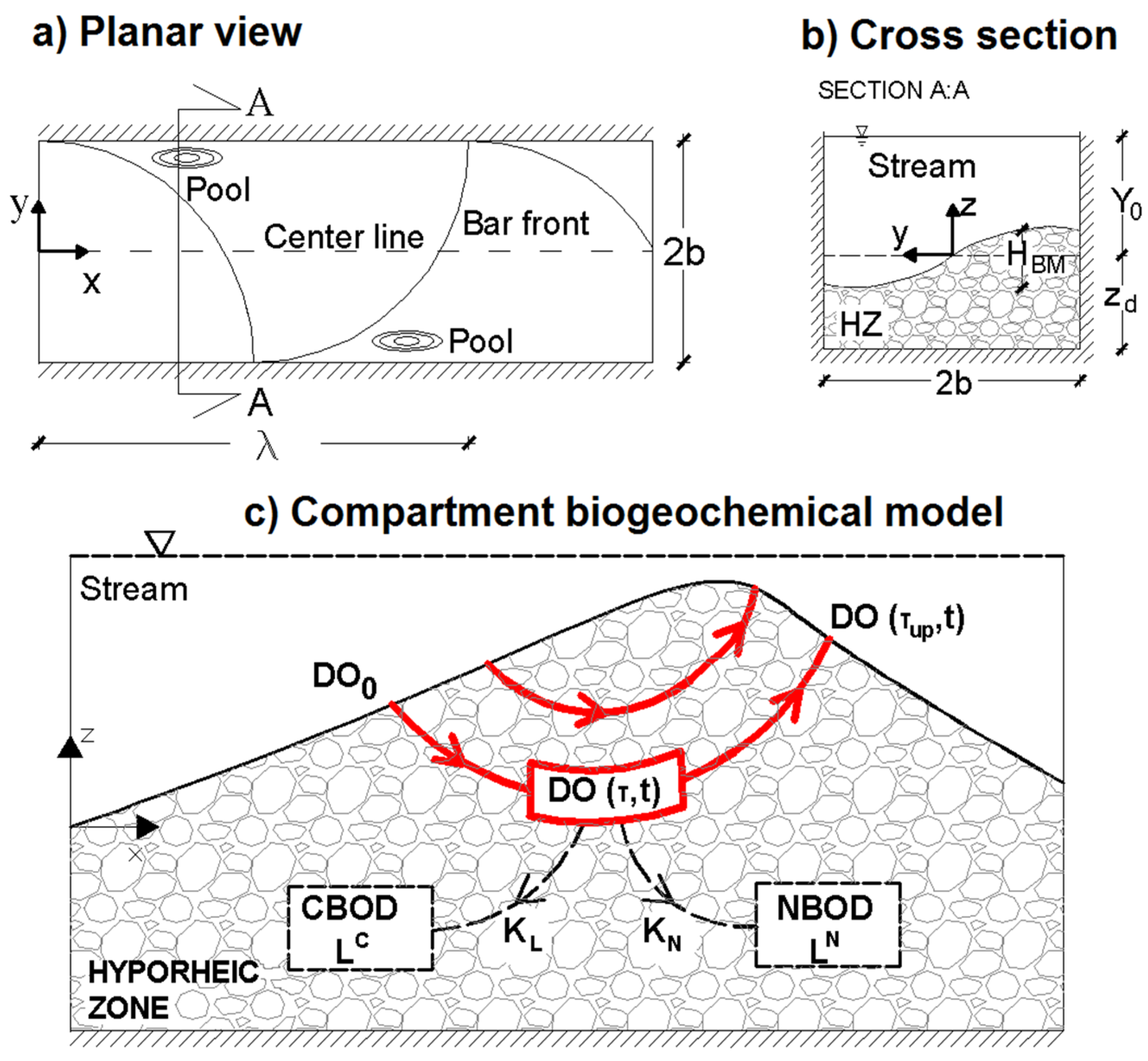
2.1. Hyporheic Hydraulic Model

We model the hyporheic flow as a Darcian flow [18,43], with the seepage velocity given by Darcy’s law: u = −K_h∇h/n, where K_h is the hydraulic conductivity, n is the sediment porosity and h is the energy head. We assume homogenous and isotropic hydraulic properties of the streambed sediment with stationary flow conditions, such that the governing equation is the following:

$${\nabla }^{2}h=0$$

(1)

We solve Equation (1) for a three-dimensional alternate bar morphology under the assumptions that the lateral sides (stream banks) and the bottom of the alluvium are impervious and that the hydraulic head gradient is equal to the streambed slope. The stream water surface elevation, which approximates the energy head distribution in the case of submerged bars, is decomposed through the fast Fourier transform. Notice that water surface elevation can be either measured [35,36], obtained through numerical models [40,44] or obtained from analytical hydrodynamic solutions [18,45]. Owing to the linearity of Equation (1), the main components of the Fourier decomposition are applied separately as Dirichlet boundary conditions at the upper planar surface that delimitates the subsurface domain. Previous studies showed that replacing the streambed surface with the plane coinciding with the average streambed elevation, as done here, has little effects on the flow and residence time distributions [18,45]. The solutions obtained with the single FFT components as the boundary condition are then superimposed to obtain the final head distribution within the subsurface domain. Here, we represent the head distribution from two different sources: field measured heads reported by Malard et al. [41] over a pool-riffle unit and analytically predicted by the model of Colombini et al. [46] for the case of a fully-submerged three-dimensional alternate bar in equilibrium with the stream discharge (Figure 1).

Figure 1. Sketch of (a) the planar view and (b) the cross-section of the three-dimensional alternate bar morphology; and (c) diagram of the biogeochemical model. DO, dissolved oxygen; CBOD, carbonaceous biological oxygen demand; NBOD, nitrogenous biological oxygen demand.

Figure 1. Sketch of (a) the planar view and (b) the cross-section of the three-dimensional alternate bar morphology; and (c) diagram of the biogeochemical model. DO, dissolved oxygen; CBOD, carbonaceous biological oxygen demand; NBOD, nitrogenous biological oxygen demand.

Once the flow field is known, the transport equation is solved by means of the particle tracking technique [47]. The works of Marzadri et al. [45,48] on pool-riffle-induced hyporheic flow show that residence time distributions and biogeochemical transformations depend on bedform size through the ratio $Y_{BM}^{*}$ = H_BM/Y₀ between the bedform amplitude H_BM and the water hydraulic depth, Y₀.

2.2. Biogeochemical Model

Following the approach of Marzadri, et al. [31], the governing equation for DO transport within the hyporheic zone is written in a Lagrangian framework by applying mass conservation along a stream tube [49]:

$$\frac{\partial DO}{\partial \text{t}}+\frac{\partial DO}{\partial \text{τ}}=\text{α }{\nabla }^{2}DO-K_L{L}^C-K_N{L}^N-K_{R}DO$$

(2)

where α = D/u² is the ratio between the longitudinal diffusion coefficient (D) and the module square of the mean velocity (u²) (u = |u|). In addition, K_L, K_N and K_R are the (linear) reaction rates of carbonaceous BOD, nitrogenous BOD and respiration, respectively (Figure 1c). The linear reaction rates of the consumption of DO are used, owing to its relatively low concentration. The last term on the right-hand side of Equation (2) accounts for dissolved oxygen consumption due to other biological sources besides the downwelling carbonaceous and nitrogenous BODs. The model neglects the lateral exchange of mass between adjacent stream tubes, and the reaction rates are assumed to be temperature dependent. Because the effects of daily temperature oscillations are small on the biogeochemical response of the hyporheic zone at the bedform scale [50], reaction rates are assumed to change with the mean daily temperature, according to the Arrhenius law [51].

We assume full mixing within the stream, such that the solute concentrations are spatially constant within the downwelling surface, while they vary in time. The initial zero concentration of all solutes is assumed within the hyporheic zone. With these hypotheses, we solve Equation (2) for constant and sinusoidally varying DO, L^C and L^N stream water concentrations. The latter assumption derives from experimental results showing that daily variations of nutrient concentrations are well approximated by a sinusoidal function [13]. Solutions of Equation (2) under these initial and boundary conditions are reported in Appendix A.

We introduce two dimensionless numbers: the first is the ratio between the dissolved oxygen concentration in the stream water, DO₀, and the total oxygen demand (L₀^C + L₀^N), R_DO = DO₀/(L₀^C + L₀^N), and the second is the ratio between carbonaceous and nitrogenous BOD concentrations, R_BN = L₀^C/L₀^N, with the objective to facilitate the analysis of the effects of nutrient loads on BUR.

2.3. Benthic Uptake Rate

BUR is defined as the difference between mass fluxes of DO entering and leaving the streambed sediments, which are given by the first and the second term on the right-hand side of Equation (3), respectively:

$$BUR=\frac{1}{{\text{τ}}_{max}}\left[{\displaystyle \underset{t_0}{\overset{t_0+{\text{τ}}_{max}}{\int }}\frac{1}{A}{\displaystyle \underset{-b}{\overset{b}{\int }}{\displaystyle \underset{0}{\overset{\text{λ}}{\int }}H\left(x,y\right)q\left(x,y\right)D{O}_0}}\left(t\right)dxdydt}-{\displaystyle \underset{t_0}{\overset{t_0+{\text{τ}}_{max}}{\int }}\frac{1}{A}{\displaystyle \underset{-b}{\overset{b}{\int }}{\displaystyle \underset{0}{\overset{\text{λ}}{\int }}H\left(x,y\right)q\left(x,y\right)DO\left(\text{τ}\left(x,y\right),t\right)}}dxdy}dt\right]$$

(3)

where A = 2 b λ is the streambed area, τ(x,y) is the hyporheic residence time for a particle downwelling at x, y, z = 0 and upwelling after the (residence) time τ since injection, λ is the bedform wavelength (the distance between two pools) and 2b the width of the channel. The time τ_max is the maximum hyporheic residence time for the given bedform and defines the time interval over which BUR is quantified. In addition, t₀ is the initial time, which is set to a value larger than maximum residence time τ_max in order to eliminate in Equation (3) the effect of the initial conditions. The step function H is unitary within the downwelling areas and is zero outside. Notice that mass balance along a single streamline has been used in the second right-hand term of Equation (3) to transform the integral over the upwelling area in an equivalent integral over the downwelling area [31,35], under the assumption that hyporheic flow is at the steady state. The steady-state flow condition allows us to rewrite Equation (3) in the following form:

$$\begin{array}{l}BUR={\overline{DO}}_0\overline{q}-\frac{1}{2b\text{\hspace{0.17em}λ}}{\displaystyle \underset{-b}{\overset{b}{\int }}{\displaystyle \underset{0}{\overset{\text{λ}}{\int }}H(x,y)q\left(x,y\right)\overline{DO}\left(\text{τ}\left(x,y\right)\right)}}dxdy\\ \overline{q}=\frac{1}{2b\text{\hspace{0.17em}λ}}{\displaystyle \underset{-b}{\overset{b}{\int }}{\displaystyle \underset{0}{\overset{\text{λ}}{\int }}H(x,y)q\left(x,y\right)}}dxdy\end{array}$$

(4)

where $\overline{q}$ is the mean downwelling flux averaged over the entire streambed area, and time averaged dissolved oxygen concentrations are defined as:

$${\overline{DO}}_0=\frac{1}{{\tau }_{\max }}{\displaystyle \underset{t_0}{\overset{t_0+{\tau }_{\max }}{\int }}D{O}_0(t)dt}$$

(5)

and:

$$\overline{DO}(\tau )=\frac{1}{{\tau }_{\max }}{\displaystyle \underset{t_0}{\overset{t_0+{\tau }_{\max }}{\int }}DO(\tau ,t)dt}$$

(6)

at the downwelling and upwelling areas, respectively.

Because the objective of the present analysis is to quantify the contribution of the hyporheic zone to the consumption of stream DO, we make the BUR dimensionless with the mean DO mass flux in the stream:

$$BU{R}^{\ast }=\frac{2b\lambda BUR}{\frac{1}{{\tau }_{\max }}{\displaystyle \underset{t_0}{\overset{t_0+{\tau }_{\max }}{\int }}D{O}_0(t)Q_{stream}dt}}=\frac{2b\lambda BUR}{Q_{stream}\overline{D{O}_0}}$$

(7)

where Q_stream is the stream discharge. Similarly, the BUR can be made dimensionless with respect to the hyporheic flux by replacing in Equation (7) Q_stream with $\overline{q}$ A:

$$BU{R}_{HZ}^{\ast }=\frac{BUR}{\overline{q}{\overline{DO}}_0}$$

(8)

Hereafter, this dimensionless expression of BUR will be indicated with ${BUR}_{HZ}^{*}$.

The following two end members can be defined for BUR^* when all of the upwelling fluxes are anoxic, such that all of the oxygen carried by the stream is consumed within the hyporheic zone:

$$\begin{array}{l}BU{R}^{\ast }=\frac{\overline{q}2b\lambda }{Q_{stream}}for{R}_{DO}<1\\ BU{R}^{\ast }=R_{DO}^{-1}\frac{\overline{q}2b\lambda }{Q_{stream}}for{R}_{DO}>1\end{array}$$

(9)

which have been obtained by considering that carbonaceous and nitrogen oxygen consumption is limited by the DO of stream water, such that $BUR=\overline{q} \overline{D{O}_0}$ when RD₀ < 1 and BUR = L₀^C + L₀^N when RD₀ > 1. Equation (8) provides a first approximation analysis for BUR^*, which depends only on the hyporheic ($\overline{q}$ 2bλ) and stream (Q_stream) discharges, the hyporheic residence time distribution and the nutrient loads (R_DO = DO₀/(L₀^C + L₀^N)) in the stream. The hyporheic values, τ_max and $\overline{q}$, can be estimated with models presented in the literature [18,19,45,52,53,54,55].

2.4. Field Data

The works of Malard et al. [41] and Rouch [42] report both the near-bed head and the dissolved oxygen concentration distributions at the sediment-water interface, supplemented by streambed sediment hydraulic conductivity and porosity along a 15 m-long pool-riffle bar reach of the Lachein stream (Pyrennees, France). In the present work, the head distribution derived from the contour lines depicted in Figure 3c of Malard et al. [41] by superimposing a regular two-dimensional grid is first decomposed via FFT (Figure 2). Owing to the linearity of the flow Equation (1) and Darcy’s law, the most relevant FFT components are used as the upper Dirichlet boundary condition for modeling the 3D hyporheic flow field, through the solution of Laplace and Darcy equations, separately for each component, under the assumption of homogeneous and isotropic alluvium, as described in Section 2.1. The resulting velocity fields are then superimposed to obtain the final three-dimensional velocity field distribution. We set the alluvium thickness to z_d = 2 m, which is deep enough to make negligible its effect on the hyporheic flow field, the hydraulic conductivity to K_h = 8.39 × 10⁻⁴ m/s, which is the mean of the hydraulic conductivity values reported in Figure 3b of Malard et al. [41], and the porosity to n = 0.2664, which is the mean of the porosity values reported by Rouch [42] for this study site. The residence time of 8192 particles injected within the downwelling area was obtained by particle tracking with the analytical velocity obtained as explained above. We do not account for particles whose trajectories do not upwell in the stream.

Figure 2. Head distribution in the 15 m-long reach of the Lachein stream measured by Malard et al.’s [41] contour lines and reconstructed by FFT (color plot).

Figure 2. Head distribution in the 15 m-long reach of the Lachein stream measured by Malard et al.’s [41] contour lines and reconstructed by FFT (color plot).

For the biogeochemical model, we assumed a constant dissolved oxygen concentration in the stream water, DO₀ = 10 mg/L, which is the mean of the measured values over the downwelling areas, and a saturated DO concentration of DO_sat = 11.83 mg/L, which corresponds to the observed water temperature of T = 8 °C. In addition, we set the reaction rate of respiration equal to the mean value calculated from the field data reported by Beaulieu et al. [56] for streams with a water temperature near 20 °C: K_R(20 °C) = 5.01 d⁻¹. We neglect all of the other parameters, DO_lim, L^C, L^N and α, whose values were not reported in the work of Malard et al. [41] and Rouch [42]. The coefficient K_R implicitly accounts for the consumption of DO due to both carbonaceous and nitrogenous BOD, whose values were not reported, and thus, we set K_L and K_N equal to 0. These working assumptions allow us to use only measured values, avoiding the need to calibrate the model.

We used the error matrix technique, which is a common GIS (Geographic Information System) method for map comparison [57,58,59], to assess the accuracy of the modeled spatially-distributed DO concentrations against field observations. The error matrix provides two indexes of agreement between predicted and observed spatially-distributed quantities on a cell-by-cell basis: an overall agreement, OA, and a kappa index. The OA is calculated as the proportion of correctly-predicted cells versus the total number of cells. Differently from OA, the kappa index removes the effect of by-chance agreement. In fact, the probability that two successive random extractions of a categorical variable belong to the same category is larger than zero, by definition. Since the kappa index filters out the match of predicted and observed DO cells due to random coincidence, its value is typically lower than OA [60]. Both indexes vary from 0 to 1 with 0 being poor and 1 perfect agreement. For the K statistic, Landis and Koch [59] suggested the following classification: <0 = poor agreement, 0–0.19 slight, 0.20–0.39 fair, 0.4–0.59 moderate, 0.60–0.79 substantial and 0.80–1.00 almost perfect agreement. We calculated OA and K with the DO concentrations divided into the 3 categories reported by Malard et al. [41]. The predicted and observed DO category needs to coincide exactly to be counted as a match and not an error. This is a strict method, because it does not take into account if the match is a little bit offset spatially; for instance, a nearby cell could have the correct value [60].

2.5. Numerical Simulations

We considered 18 streams characterized by an alternate bar morphology, whose bedforms are in equilibrium with the flow discharge. The bedform dimensions, whose morphodynamic parameters are reported in Table 1, are within those typically encountered in natural streams [39,61,62,63]. For each stream, we ran 10 simulations, changing the nutrient loads (Table 2). We ran a set of simulations with constant loads and a set with sinusoidal varying CBOD, NBOD and DO concentrations with the same mean value as the constant case to explore the effects of time-dependent nutrient releases.

Table 1. Morphodynamic parameters of the pool-riffle bedform. β is the aspect ratio (β = b/Y₀); θ is the Shields’ number; d_s is the relative submergence of the particles; d₅₀ is the median grain size; $Y_{BM}^{*}$ is the dimensionless mean flow depth; s is the streambed slope; ∆ is the bar amplitude; λ is the bar length; and Q_stream is the stream water discharge.

Test	β (-)	θ (-)	dS (-)	d50 (m)	$Y_{BM}^{*}$ (-)	S (%)	HBM (m)	λ (m)	Qstream (m3·s−1)
1	13	0.08	0.200	0.01	0.33	2.64	0.15	8.76	0.057
2	13	0.08	0.150	0.01	0.39	1.98	0.17	11.52	0.111
3	13	0.08	0.120	0.01	0.45	1.58	0.19	14.23	0.185
4	13	0.08	0.105	0.01	0.48	1.39	0.20	16.16	0.251
5	13	0.08	0.095	0.01	0.50	1.25	0.21	17.77	0.314
6	13	0.08	0.085	0.01	0.53	1.12	0.22	19.75	0.404
7	13	0.08	0.075	0.01	0.56	0.99	0.23	22.26	0.537
8	13	0.08	0.065	0.01	0.60	0.86	0.26	25.53	0.738
9	13	0.08	0.060	0.01	0.62	0.79	0.27	27.57	0.883
10	13	0.08	0.055	0.01	0.65	0.73	0.28	29.98	1.072
11	13	0.08	0.050	0.01	0.68	0.66	0.29	32.87	1.325
12	13	0.08	0.045	0.01	0.71	0.59	0.31	36.40	1.675
13	13	0.08	0.040	0.01	0.75	0.53	0.33	40.82	2.174
14	13	0.08	0.035	0.01	0.81	0.46	0.33	46.52	2.902
15	13	0.08	0.030	0.01	0.87	0.40	0.38	54.13	4.101
16	13	0.08	0.025	0.01	0.96	0.33	0.42	64.82	6.121
17	13	0.08	0.020	0.01	1.08	0.26	0.46	80.97	9.977
18	13	0.08	0.010	0.01	1.74	0.13	0.56	163.14	45.037

Table 1. Morphodynamic parameters of the pool-riffle bedform. β is the aspect ratio (β = b/Y₀); θ is the Shields’ number; d_s is the relative submergence of the particles; d₅₀ is the median grain size; $Y_{BM}^{*}$ is the dimensionless mean flow depth; s is the streambed slope; ∆ is the bar amplitude; λ is the bar length; and Q_stream is the stream water discharge.

Test	β (-)	θ (-)	dS (-)	d50 (m)	$Y_{BM}^{*}$ (-)	S (%)	HBM (m)	λ (m)	Qstream (m3·s−1)
1	13	0.08	0.200	0.01	0.33	2.64	0.15	8.76	0.057
2	13	0.08	0.150	0.01	0.39	1.98	0.17	11.52	0.111
3	13	0.08	0.120	0.01	0.45	1.58	0.19	14.23	0.185
4	13	0.08	0.105	0.01	0.48	1.39	0.20	16.16	0.251
5	13	0.08	0.095	0.01	0.50	1.25	0.21	17.77	0.314
6	13	0.08	0.085	0.01	0.53	1.12	0.22	19.75	0.404
7	13	0.08	0.075	0.01	0.56	0.99	0.23	22.26	0.537
8	13	0.08	0.065	0.01	0.60	0.86	0.26	25.53	0.738
9	13	0.08	0.060	0.01	0.62	0.79	0.27	27.57	0.883
10	13	0.08	0.055	0.01	0.65	0.73	0.28	29.98	1.072
11	13	0.08	0.050	0.01	0.68	0.66	0.29	32.87	1.325
12	13	0.08	0.045	0.01	0.71	0.59	0.31	36.40	1.675
13	13	0.08	0.040	0.01	0.75	0.53	0.33	40.82	2.174
14	13	0.08	0.035	0.01	0.81	0.46	0.33	46.52	2.902
15	13	0.08	0.030	0.01	0.87	0.40	0.38	54.13	4.101
16	13	0.08	0.025	0.01	0.96	0.33	0.42	64.82	6.121
17	13	0.08	0.020	0.01	1.08	0.26	0.46	80.97	9.977
18	13	0.08	0.010	0.01	1.74	0.13	0.56	163.14	45.037

Table 2. Biogeochemical parameters used in the simulations. R_DO is the ratio between dissolved oxygen concentration (DO) and the total oxygen demand; R_BN is the ratio between carbonaceous (L^C) and nitrogenous (L^N) BOD; L₀^C and L₀^N are the constant stream concentrations of carbonaceous (CBOD) and nitrogenous (NBOD) BOD, respectively. L_A^C and L_A^N are the stream daily fluctuations of CBOD and NBOD, respectively. K_L, K_N and K_R are the decay rates of CBOD, NBOD and DO, respectively. In all of the simulations, the concentration of dissolved oxygen concentration DO₀ = 10 mg/L, while the stream daily fluctuation of oxygen is DO_A = 4 mg/L.

Test	RDO (-)	RBN (-)	L0C (mg/L)	LAC (τ,0) (mg/L)	L0N (mg/L)	LAN (τ,0) (mg/L)	KL (d−1)	KN (d−1)	KR (d−1)
A	1.2	0.5	2.78	1.11	5.56	2.22	0.33	0.26	0.16
B	1.0	0.5	3.33	1.33	6.67.	2.67	0.33	0.26	0.16
C	0.8	0.5	4.16	1.67	8.32	3.33	0.33	0.26	0.16
D	0.5	0.5	6.67	2.67	13.33	5.33	0.33	0.26	0.16
E	0.2	0.5	16.66	6.67	33.33	13.33	0.33	0.26	0.16
F	1.2	2.0	5.56	2.22	2.78	1.11	0.33	0.26	0.16
G	1.0	2.0	6.67	2.67	3.33	1.33	0.33	0.26	0.16
H	0.8	2.0	8.32	3.33	4.16	1.67	0.33	0.26	0.16
I	0.5	2.0	13.34	5.33	6.67	2.67	0.33	0.26	0.16
J	0.2	2.0	33.33	13.33	16.67	6.67	0.33	0.26	0.16

Table 2. Biogeochemical parameters used in the simulations. R_DO is the ratio between dissolved oxygen concentration (DO) and the total oxygen demand; R_BN is the ratio between carbonaceous (L^C) and nitrogenous (L^N) BOD; L₀^C and L₀^N are the constant stream concentrations of carbonaceous (CBOD) and nitrogenous (NBOD) BOD, respectively. L_A^C and L_A^N are the stream daily fluctuations of CBOD and NBOD, respectively. K_L, K_N and K_R are the decay rates of CBOD, NBOD and DO, respectively. In all of the simulations, the concentration of dissolved oxygen concentration DO₀ = 10 mg/L, while the stream daily fluctuation of oxygen is DO_A = 4 mg/L.

Test	RDO (-)	RBN (-)	L0C (mg/L)	LAC (τ,0) (mg/L)	L0N (mg/L)	LAN (τ,0) (mg/L)	KL (d−1)	KN (d−1)	KR (d−1)
A	1.2	0.5	2.78	1.11	5.56	2.22	0.33	0.26	0.16
B	1.0	0.5	3.33	1.33	6.67.	2.67	0.33	0.26	0.16
C	0.8	0.5	4.16	1.67	8.32	3.33	0.33	0.26	0.16
D	0.5	0.5	6.67	2.67	13.33	5.33	0.33	0.26	0.16
E	0.2	0.5	16.66	6.67	33.33	13.33	0.33	0.26	0.16
F	1.2	2.0	5.56	2.22	2.78	1.11	0.33	0.26	0.16
G	1.0	2.0	6.67	2.67	3.33	1.33	0.33	0.26	0.16
H	0.8	2.0	8.32	3.33	4.16	1.67	0.33	0.26	0.16
I	0.5	2.0	13.34	5.33	6.67	2.67	0.33	0.26	0.16
J	0.2	2.0	33.33	13.33	16.67	6.67	0.33	0.26	0.16

These simulations are tailored to investigate the relationship between BUR^*, R_BN and R_DO, which identify the nutrient loads, and $Y_{BM}^{*}$, an index of stream size. Large streams are typically characterized by large Y^*_BM and long residence times, whereas small streams by small Y^*_BM and short residence times [31].

3. Results and Discussion

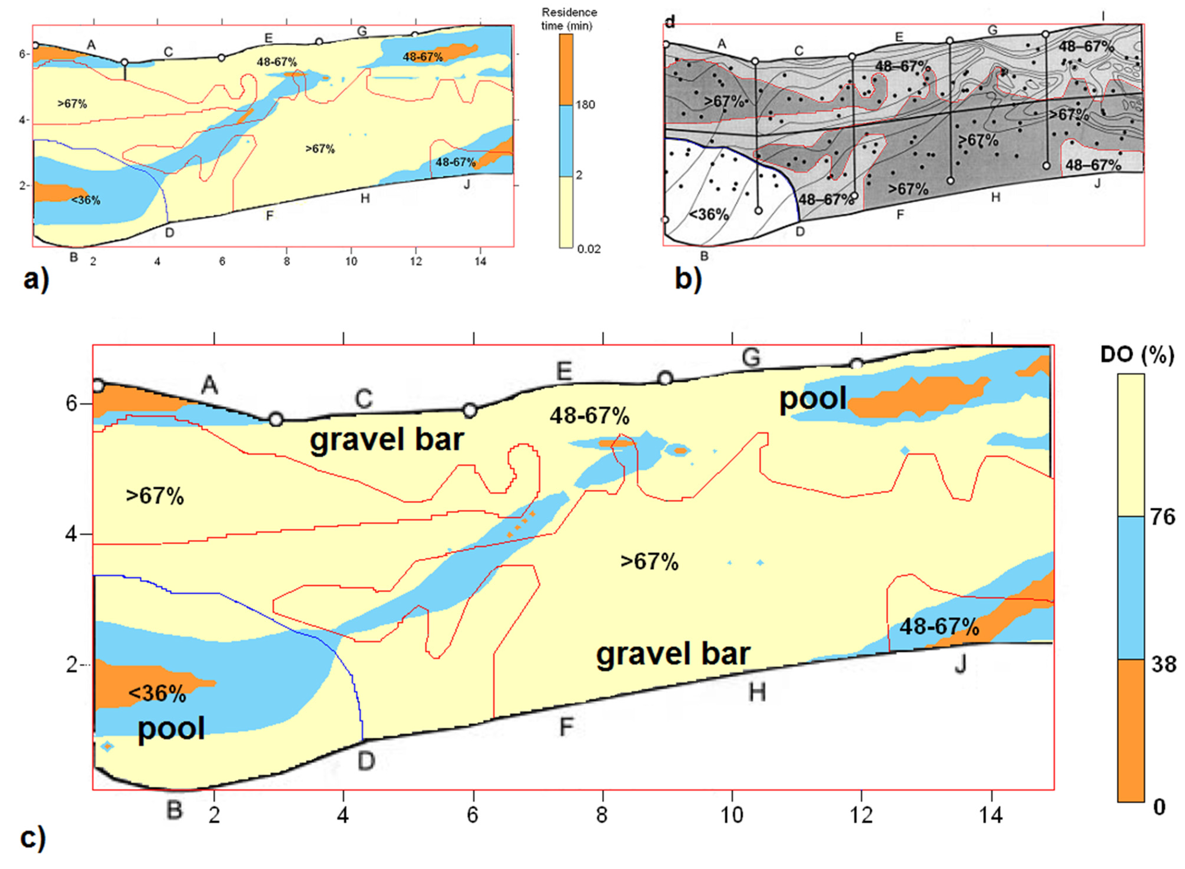
3.1. Comparison with Field Data

Figure 3 shows the contour map of the computed hyporheic residence times (Figure 3a), the categorical map of measured dissolved oxygen concentration (red contours) (Figure 3b, which corresponds to Figure 4d in Malard et al. [41]) and the map of model-predicted dissolved oxygen concentrations (Figure 3c) at the sediment-water interface. The overall agreement value between the predicted and observed DO concentration distribution is 0.58, and the kappa index is 0.46, which correspond to a good agreement and are comparable to the values reported in the GIS literature [57,59,64]. Because, to our knowledge, this is the first comparison between observed and modeled spatially-distributed hyporheic quantities, we cannot compare these values with others reported in the hyporheic literature. This result indicates that hyporheic processes are those that chiefly control the DO concentration distribution at and below the water-sediment interface and, consequently, affect the habitat of benthic and hyporheos organisms. The predicted patterns of τ and DO concentrations also match the contours of the categorical map of DO concentrations measured in the field (Figure 4d in [41]). This further confirms that residence time distribution is a key factor in the fate of reactive solutes within the hyporheic zone. In our case, the transformations depend entirely on the reaction time, because the biogeochemical reaction rates are spatially and temporally constant.

Figure 3. Maps of: (a) the computed residence time distribution of water within the hyporheic zone, τ_up; (b) the measured dissolved oxygen concentrations, (DO), in % of saturation reproduced from Figure 4d in Malard et al. [41]; and (c) the model-predicted DO along the 15-m reach of the Lachein stream.

Figure 3. Maps of: (a) the computed residence time distribution of water within the hyporheic zone, τ_up; (b) the measured dissolved oxygen concentrations, (DO), in % of saturation reproduced from Figure 4d in Malard et al. [41]; and (c) the model-predicted DO along the 15-m reach of the Lachein stream.

Malard et al. [41] observed that organisms colonized preferential areas of the streambed depending on DO concentrations and described the behavior in terms of morphological units: bar, pool and bar fringe. Patches with a high dissolved oxygen concentration (>74% of saturation) coincide with depositional areas, such as bars, which are mostly predicted as downwelling zones, and bar fringes, which are predicted as upwelling areas with a short residence time. These zones show dense communities of harpacticoid and hypogean species; whereas streambed areas with low DO concentrations, which are identified as erosional areas by Malard et al. [41], like the pool, and for which our model predicts upwelling areas with long residence times, have fewer harpacticoids and hypogean organisms. All of these results suggest that the near-bed DO concentration is chiefly controlled by stream bedforms, which therefore control the habitat within and at the streambed sediment.

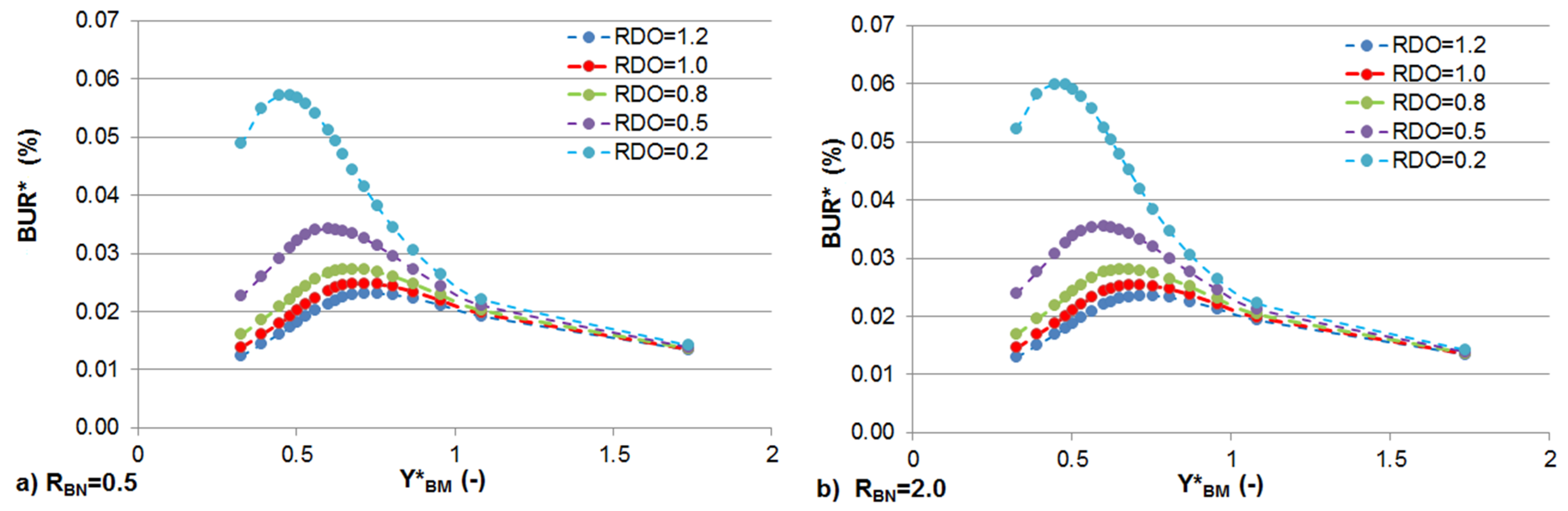
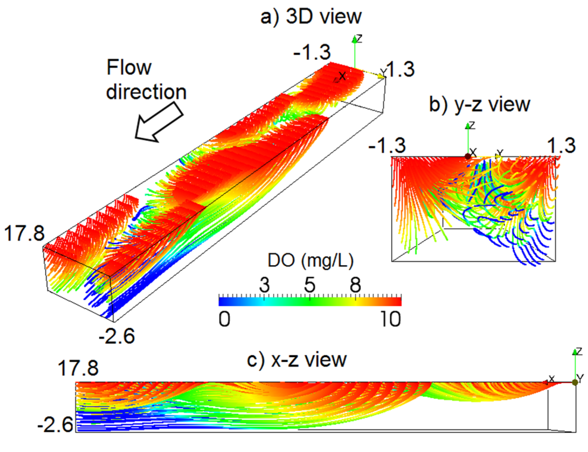
3.2. Effect of Stream Morphology

Figure 4a shows BUR^*, i.e., the BUR made dimensionless with respect to the stream flux, as a function of the dimensionless depth, Y^*_BM, for hyporheic zones induced by three-dimensional pool-riffle morphology for R_DO = 1.2 and R_BN = 0.5. In addition, Figure 4b shows how the BUR (${BUR}_{\mathrm{H}\mathrm{Z}}^{*}$) behaves when it is normalized with respect to the hyporheic flux.

Figure 4. (a) Stream, BUR^*, and (b) hyporheic, BUR^*_HZ, dimensionless BUR, as a function of dimensionless mean flow depth, $Y_{BM}^{*}$, for three-dimensional alternate bars with R_DO = 1.2 and R_BN = 0.5, with R_DO being the ratio between in-stream DO (DO₀) and total oxygen demand (L₀^C + L₀^N) and R_BN the ratio between in-stream carbonaceous and nitrogenous BOD concentrations, R_BN = L₀^C/L₀^N. BUR, benthic uptake rate.

Figure 4. (a) Stream, BUR^*, and (b) hyporheic, BUR^*_HZ, dimensionless BUR, as a function of dimensionless mean flow depth, $Y_{BM}^{*}$, for three-dimensional alternate bars with R_DO = 1.2 and R_BN = 0.5, with R_DO being the ratio between in-stream DO (DO₀) and total oxygen demand (L₀^C + L₀^N) and R_BN the ratio between in-stream carbonaceous and nitrogenous BOD concentrations, R_BN = L₀^C/L₀^N. BUR, benthic uptake rate.

BUR^* initially increases with river size: it reaches a peak and then decreases for large streams. The peak for BUR^* is caused by the initial faster increase of downwelling fluxes with long hyporheic residence times, which potentially allow more DO consumption, than stream discharge, which also increases with stream size [54]. Eventually, the increase in stream discharge is large enough to offset the increase in hyporheic exchange, such that BUR^* decreases.

Differently from BUR^*, BUR^*_HZ increases monotonically with river size, because of the longer residence time that water spends within the hyporheic zone as the size of the river increases. Whereas the BUR^*_HZ increase is fast around Y^*_BM = 1, it slows down significantly at larger values of Y^*_BM. This suggests that short flow paths may be always present, reducing the efficiency of the hyporheic zone to consume DO to a value smaller than 100%, even for large streams.

Figure 5 shows a snapshot of hyporheic DO concentrations along the streamlines of the 3D hyporheic flow field provided by our model. Within the alluvium, the concentration of DO decreases with depth according to the time that water spends traveling along a given streamline.

The longer the path is, the greater is the probability to find streamlines with DO < 2 mg/L (red path of the trajectory) and, thus, volumes of sediment in anaerobic conditions. The complex DO distribution depicted in Figure 5 demonstrates the importance of considering the entire three-dimensional flow patterns when studying alternate bar morphologies. As the stream dimension increases, the volume of streambed sediment saturated with stream water by the hyporheic flow increases and, consequently, so do the residence times. Thus, in large streams, the red portion of the flow lines would dominate. However, the presence of short residence times at the transitional zone between upwelling and downwelling areas would still have a blue tone. This supports the results of Figure 4, which suggest that ${BUR}_{\mathrm{H}\mathrm{Z}}^{*}$ may be limited to a value below 100%. However, this upper threshold depends also on biogeochemical rates, because faster rates would require shorter times to reach anoxic conditions [32,65].

Figure 5. Snapshot of dissolved oxygen concentrations (DO) simulated within the hyporheic zone of a river with the morphological parameters of Test 5 in Table 1.

Figure 5. Snapshot of dissolved oxygen concentrations (DO) simulated within the hyporheic zone of a river with the morphological parameters of Test 5 in Table 1.

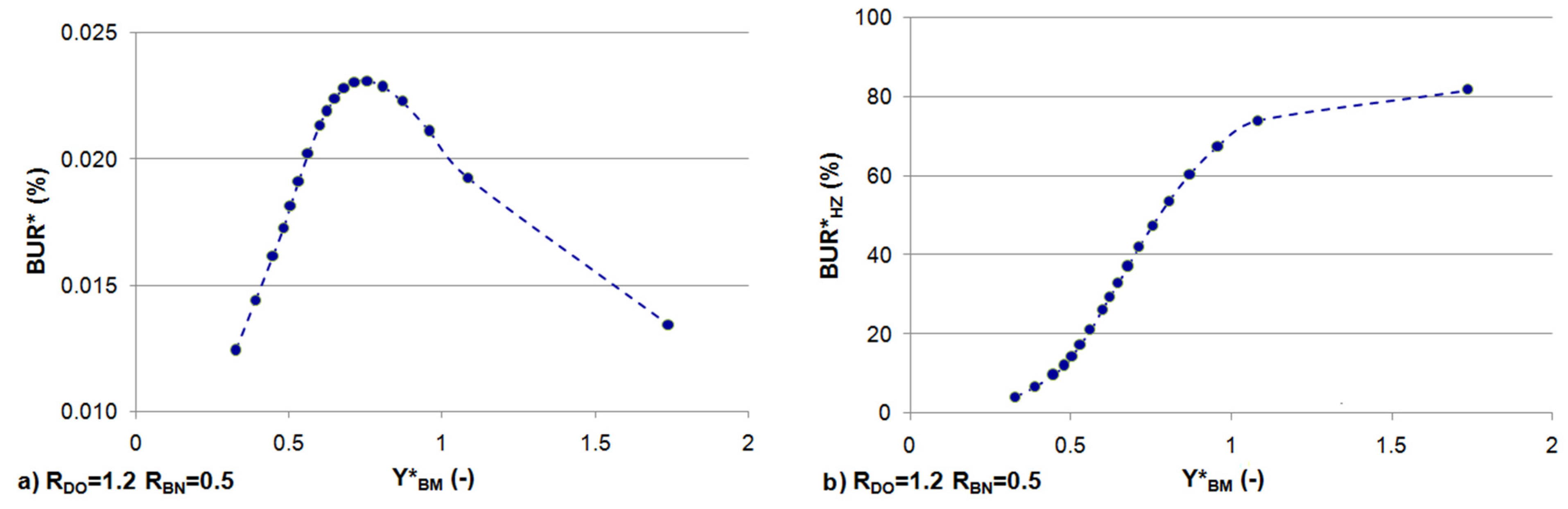
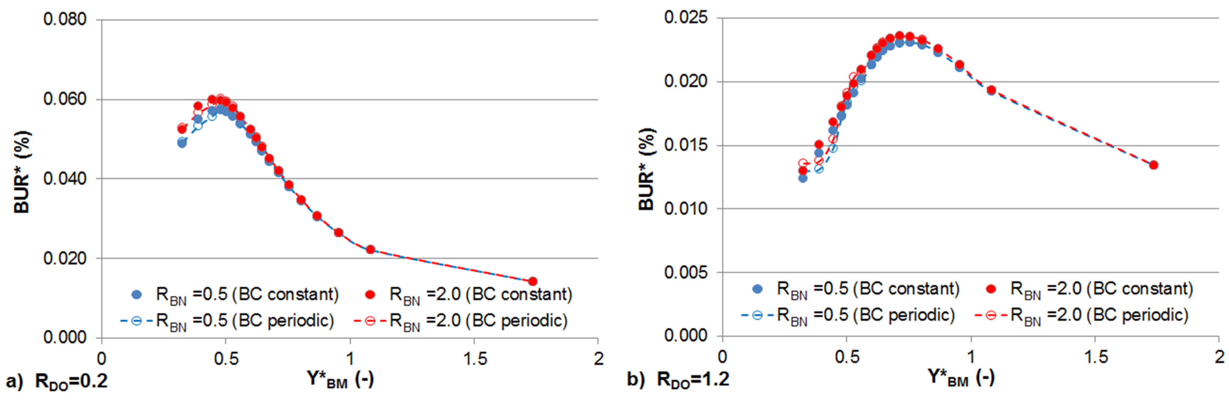
3.3. Effects of Constant BOD and DO Loads

Figure 6 shows BUR^* as a function of $Y_{BM}^{*}$ in the case of three-dimensional alternate bars for several R_DO values with R_BN = 0.5 (Figure 6a) and R_BN = 2 (Figure 6b). Keeping in mind the discussion in Section 3.2 concerning the mechanism leading to the peak in the BUR^* (Figure 4a), here, we can observe the effect of nutrient concentrations on the location of this peak. In particular, as R_DO decreases (because stream DO decreases or L₀^C + L₀^N increases), the total oxygen demand (L^C + L^N) is larger than the stream DO concentrations; the BUR^* peak increases, and it occurs in smaller streams (smaller $Y_{BM}^{*}$) for low rather than high R_DO. For instance, the BUR^* peak occurs at $Y_{BM}^{*}$ = 0.75 for R_DO = 1.2 and at Y^*_BM = 0.48 for R_DO = 0.2, regardless of R_BN. Both cases with a different R_BN show similar patterns with slightly higher BUR^* associated with larger R_BN. The faster kinetics of L^C than L^N justifies this behavior.

Figure 6. Dimensionless stream BUR, BUR^*, as a function of the dimensionless mean flow depth, $Y_{BM}^{*}$, and R_DO for (a) R_BN = 0.5 and (b) R_BN = 2.0, with R_DO the ratio between in-stream DO (DO₀) and total oxygen demand (L₀^C + L₀^N) and R_BN the ratio between in-stream carbonaceous and nitrogenous BOD concentrations, R_BN = L₀^C/L₀^N.

Figure 6. Dimensionless stream BUR, BUR^*, as a function of the dimensionless mean flow depth, $Y_{BM}^{*}$, and R_DO for (a) R_BN = 0.5 and (b) R_BN = 2.0, with R_DO the ratio between in-stream DO (DO₀) and total oxygen demand (L₀^C + L₀^N) and R_BN the ratio between in-stream carbonaceous and nitrogenous BOD concentrations, R_BN = L₀^C/L₀^N.

However, the effect of nutrient loads on BUR^* is important only for small streams. As the stream size increases, both the R_DO and R_BN effects become negligible, and all curves tend to the same value. Our simulation suggests that the threshold is near $Y_{BM}^{*}$ = 1.

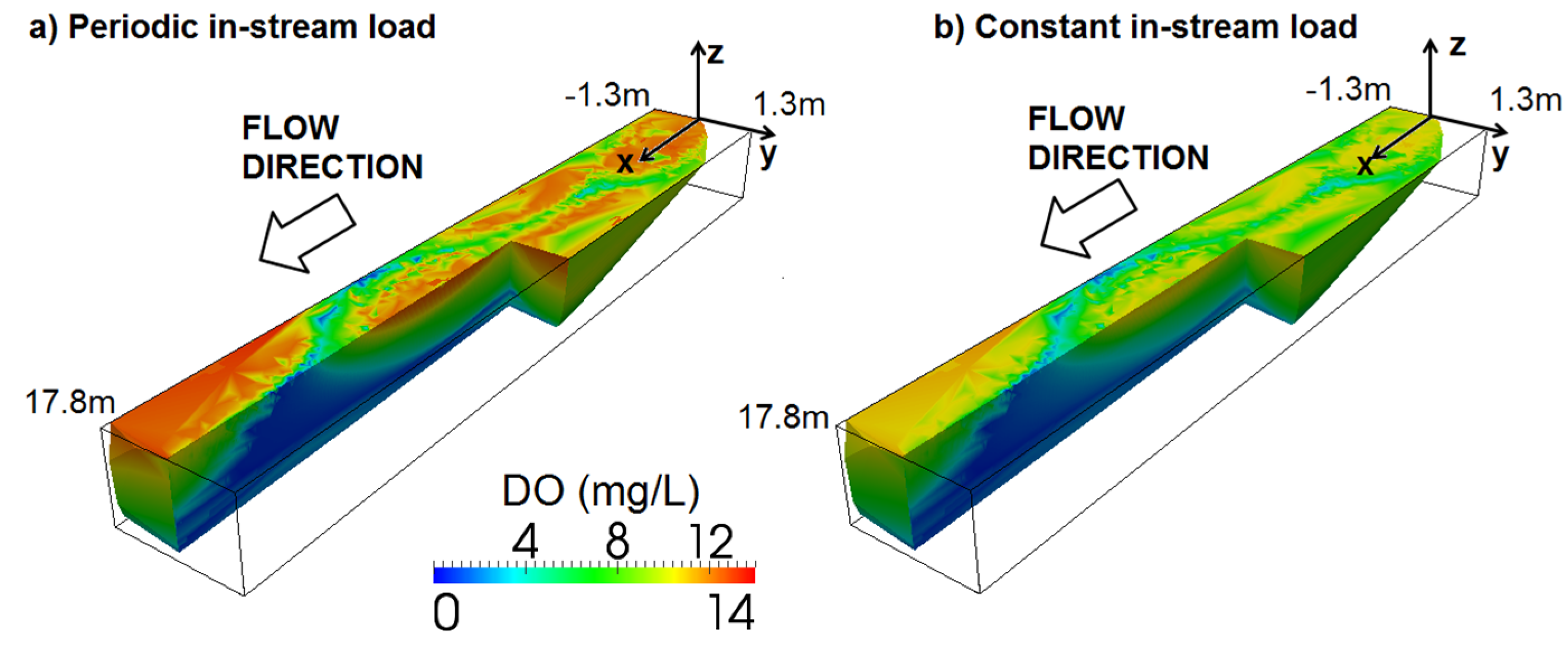
3.4. Effects of Sinusoidally Varying and Constant Stream Solute Concentrations

Figure 7 shows BUR^* for sinusoidally varying and constant L^C and L^N loads as a function of $Y_{BM}^{*}$ for R_BN = 0.5 with R_DO = 0.2 (Figure 7a) and R_DO = 1.2 (Figure 7b). The most important result shown in Figure 7a,b is that including daily variations of the stream DO provides little benefit with respect to the use of a constant stream DO for large streams. Some effects of the time-varying in-stream concentration are observed for small streams. This behavior can be explained by considering the hyporheic residence time as the main controlling factor of DO consumption for the same biological activity. Path lines with long residence times show larger portions with low DO concentrations, which are less affected by the daily DO fluctuations of stream water.

Figure 7. Dimensionless stream BUR, BUR^*, as a function of the dimensionless mean flow depth, $Y_{BM}^{*}$, for periodic and constant in-stream boundary conditions and R_BN = 0.5 with (a) R_DO = 0.2 and (b) R_DO = 1.2, with R_DO the ratio between in-stream DO (DO₀) and total oxygen demand (L₀^C + L₀^N) and R_BN the ratio between in-stream carbonaceous and nitrogenous BOD concentrations, R_BN = L₀^C/L₀^N.

Figure 7. Dimensionless stream BUR, BUR^*, as a function of the dimensionless mean flow depth, $Y_{BM}^{*}$, for periodic and constant in-stream boundary conditions and R_BN = 0.5 with (a) R_DO = 0.2 and (b) R_DO = 1.2, with R_DO the ratio between in-stream DO (DO₀) and total oxygen demand (L₀^C + L₀^N) and R_BN the ratio between in-stream carbonaceous and nitrogenous BOD concentrations, R_BN = L₀^C/L₀^N.

Conversely, large portions of path lines with short residence times show DO concentrations that vary temporally, depending on stream nutrient and DO concentrations. Thus, systems with predominantly long residence times, like streams with large $Y_{BM}^{*}$, show a similar global response for both boundary conditions; whereas the BUR^* response of streams with small Y^*_BM shows a dependence on temporal variations of stream nutrient and DO concentrations. However, as shown in Figure 7a,b, the dependence on DO fluctuations in stream water is small, yet appreciable, thereby suggesting that the mean daily concentrations of DO are sufficient information for studying the global response of the hyporheic zone in most cases of practical interest.

BUR^* shows the overall system response, which is certainly important for understanding the mean behavior of the system for different types of stream nutrient loads (Figure 7a,b). However, the lifetime of many aquatic organisms is strongly related to the local behavior of the system, which could be quite different from the overall response. In this context, Figure 8 shows a three-dimensional snapshot of simulated DO concentrations within the hyporheic zone in the case of sinusoidally-periodic (Figure 8a) and constant (Figure 8b) DO, L^C and L^N concentrations for R_DO = 1.2 and R_BN = 0.5.

Figure 8. Maps of dissolved oxygen concentrations, DO, within the hyporheic zone for (a) periodic and (b) constant in-stream concentrations of DO, CBOD and NBOD. In both cases, R_DO = 1.2 and R_BN = 0.5 (Test 5-A), with R_DO the ratio between in-stream DO (DO₀) and total oxygen demand (L₀^C + L₀^N) and R_BN the ratio between in-stream carbonaceous and nitrogenous BOD concentrations, R_BN = L₀^C/L₀^N.

Figure 8. Maps of dissolved oxygen concentrations, DO, within the hyporheic zone for (a) periodic and (b) constant in-stream concentrations of DO, CBOD and NBOD. In both cases, R_DO = 1.2 and R_BN = 0.5 (Test 5-A), with R_DO the ratio between in-stream DO (DO₀) and total oxygen demand (L₀^C + L₀^N) and R_BN the ratio between in-stream carbonaceous and nitrogenous BOD concentrations, R_BN = L₀^C/L₀^N.

The variation in time of the two nutrients and DO in the stream water induce differentiated spatial and temporal distributions of DO concentrations within the hyporheic zone. The temporal changes of DO concentrations are not systematic within the domain, but they are relevant for short residence times and become negligible along the streamlines as the residence time increases. Thus, the hyporheic zone may show a dynamic volume of sediment, whose DO concentrations fluctuate following those of the stream water, and a stable volume, where DO concentrations are low and stationary. We should expect a spatial specialization of organisms dwelling in the hyporheic zone following the DO profile as those observed at the sediment-water interface by Malard et al. [41].

4. Conclusions

We presented an analytical model, which accounts for advection, diffusion and both carbonaceous and nitrogenous BODs, for predicting DO concentrations within the hyporheic zone. The application of the model on a gravel-bed pool-riffle reach shows that the proposed semi-analytical tool is able to predict the spatial distribution of measured DO concentrations. The overall agreement between predicted and observed DO concentrations is 58%. Our results show that hyporheic DO consumption varies as a function of bedform morphology, size and nutrient loads. Our model uses spatially-constant reaction rates, which probably may change spatially, and homogenous hydraulic conductivities. These two limitations may be important to detect micro-biogeochemical hotspots, which may be linked to localized slow velocities [65].

Our simulations suggest that river morphology plays an important role in controlling the BOD removal capacity of the hyporheic zone. However, the system responds differently at local and global scales, depending on the temporal variations of stream DO concentrations. The bedform scale response of the hyporheic zone expressed by BUR^* is only minimally influenced by daily oscillations of stream water nutrient and DO concentrations. Thus, daily mean concentrations of these solutes can be used as an index for quantifying the hyporheic response at the bedform scale. Conversely, daily oscillations of stream nutrient concentrations may influence the spatial distribution and density of aquatic organisms locally. Finally, we show that for a given nutrient concentration, there is a stream size that maximizes the removal of L^C and L^N and, consequently, the consumption of stream dissolved oxygen.

References

1. Galloway, J.N.; Dentener, F.J.; Capone, D.G.; Boyer, E.W.; Howarth, R.W.; Seitzinger, S.P.; Asner, G.P.; Cleveland, C.C.; Green, P.A.; Holland, E.A.; et al. Nitrogen cycles: Past, present, and future. Biogeochemestry 2004, 70, 153–226. [Google Scholar] [CrossRef]
2. Galloway, J.N.; Townsend, A.R.; Erisman, J.W.; Bekunda, M.; Cai, Z.; Freney, J.R.; Martinelli, L.A.; Seitzinger, S.P.; Sutton, M.A. Transformation of the nitrogen cycle: Recent trends, questions, and potential solutions. Science 2008, 320, 889–892. [Google Scholar] [CrossRef] [PubMed]
3. Jelks, H.; Walsh, S.; Burkhead, N.; Contreras-Balderas, S.; Diaz-Pardo, E.; Hendrickson, D.; Lyons, J.; Mandrak, N.; McCormick, F.; Nelson, J. Conservation status of imperiled north american freshwater and diadromous fishes. Fisheries 2008, 33, 372–407. [Google Scholar] [CrossRef]
4. McMahon, P.B.; Tindall, J.A.; Collins, J.A.; Lull, K.J.; Nuttle, J.R. Hydrologic and geochemical effect on oxygen uptake in bottom sediments of an effluent-dominated river. Water Resour. Res. 1995, 31, 2561–2569. [Google Scholar] [CrossRef]
5. Paulsen, S.G.; Mayio, A.; Peck, D.; Stoddard, J.; Tarquinio, E.; Holdsworth, S.; Van Sickle, J.; Yuan, L.; Hawkins, C.; Herlihy, A.T. Condition of stream ecosystems in the us: An overview of the first national assessment. J. Inf. 2008, 27, 812–821. [Google Scholar]
6. Cooper, A.B. Activities of benthic nitrifiers in streams and their role in oxygen consumption. Microb. Ecol. 1984, 10, 317–334. [Google Scholar] [CrossRef] [PubMed]
7. Štambuk-Giljanović, N. The pollution load by nitrogen and phosphorus in the cetina river. Water Air Soil Pollut. 2010, 211, 49–60. [Google Scholar] [CrossRef]
8. Pollock, M.S.; Clarke, L.M.J.; Dubé, M.G. The effects of hypoxia on fishes: From ecological relevance to physiological effects. Environ. Rev. 2007, 15, 1–14. [Google Scholar] [CrossRef]
9. Yu, F.X.; Adrian, D.D.; Singh, V.P. Modeling river quality by the superposition method. J. Environ. Syst. 1991, 20, 1–16. [Google Scholar]
10. Rusjan, S.; Mikoš, M. Seasonal variability of diurnal in-stream nitrate concentration oscillations under hydrologically stable conditions. Biogeochemestry 2010, 97, 123–140. [Google Scholar] [CrossRef]
11. Gariglio, F.; Tonina, D.; Luce, C.H. Spatio-temporal variability of hyporheic exchange through a pool-riffle-pool sequence. Water Resour. Res. 2013, 49, 7185–7204. [Google Scholar] [CrossRef]
12. Marzadri, A.; Tonina, D.; Bellin, A. Effects of stream morphodynamics on hyporheic zone thermal regime. Water Resour. Res. 2013, 49, 2287–2302. [Google Scholar] [CrossRef]
13. Alshawabkeh, A.; Adrian, D.D. Analytical water quality model for a sinusoidally varying bod discharge concentration. Water Resour. Res. 1997, 31, 1207–1215. [Google Scholar]
14. Higashino, M.; Gantzer, C.; Stefan, H.G. Unsteady diffusional mass transfer at the sediment/water interface: Theory and significance for sod measurement. Water Res. 2004, 38, 1–12. [Google Scholar] [CrossRef] [PubMed]
15. Jorgensen, B.; Revsbech, N. Diffusive boundary layers and the oxygen uptake of sediments and detritus. Limnol. Oceanogr. 1985, 30, 111–122. [Google Scholar] [CrossRef]
16. Rutherford, I.C.; Boyle, J.D.; Elliott, A.H.; Hatherell, T.V.J.; Chiu, T.W. Modeling benthic oxygen uptake by pumping. J. Environ. Eng. 1995, 121, 84–95. [Google Scholar] [CrossRef]
17. Buffington, J.M.; Tonina, D. Hyporheic exchange in mountain rivers ii: Effects of channel morphology on mechanics, scales, and rates of exchange. Geogr. Compass 2009, 3, 1038–1062. [Google Scholar] [CrossRef]
18. Elliott, A.; Brooks, N.H. Transfer of nonsorbing solutes to a streambed with bed forms: Theory. Water Resour. Res. 1997, 33, 123–136. [Google Scholar] [CrossRef]
19. Elliott, A.; Brooks, N.H. Transfer of nonsorbing solutes to a streambed with bed forms: Laboratory experiments. Water Resour. Res. 1997, 33, 137–151. [Google Scholar] [CrossRef]
20. Tonina, D.; Buffington, J.M. Hyporheic exchange in mountain rivers i: Mechanics and environmental effects. Geogr. Compass 2009, 3, 1063–1086. [Google Scholar] [CrossRef]
21. Zarnetske, J.P.; Haggerty, R.; Wondzell, S.M.; Baker, M.A. Dynamics of nitrate production and removal as a function of residence time in the hyporheic zone. J. Geophys. Res. 2011, 116, G01025. [Google Scholar]
22. Zarnetske, J.P.; Haggerty, R.; Wondzell, S.M.; Bokil, V.A.; González-Pinzón, R. Coupled transport and reaction kinetics control the nitrate source-sink function of hyporheic zones. Water Resour. Res. 2012, 48, W11508. [Google Scholar]
23. Triska, F.J.; Duff, J.H.; Avanzino, R.J. The role of water exchange between a stream channel and its hyporheic zone in nitrogen cycling at the terrestrial-aquatic interface. Hydrobiologia 1993, 251, 167–184. [Google Scholar] [CrossRef]
24. Triska, F.J.; Duff, J.H.; Avanzino, R.J. Patterns of hydrological exchange and nutrient transformation in the hyporheic zone of a gravel bottom stream: Examining terrestrial-aquatic linkages. Freshw. Biol. 1993, 29, 259–274. [Google Scholar] [CrossRef]
25. Grimaldi, C.; Chaplot, V. Nitrate depletion during within-stream transport: Effects of exchange processes between streamwater, the hyporheic and riparian zones. Water Air Soil Pollut. 2000, 124, 95–112. [Google Scholar] [CrossRef]
26. Hlaváčová, E.; Rulík, M.; Čáp, L. Anaerobic microbial metabolism in hyporheic sediment of gravel bar in a small lowland stream. River Res. Appl. 2005, 21, 1003–1011. [Google Scholar] [CrossRef]
27. Kasahara, T.; Hill, A.R. Effects of riffle–step restoration on hyporheic zone chemistry in n-rich lowland streams. Can. J. Fish. Aquat. Sci. 2006, 63, 120–133. [Google Scholar] [CrossRef]
28. Pinay, G.; O’Keefe, T.C.; Edwards, R.T.; Naiman, R.J. Nitrate removal in the hyporheic zone of a salmon river in alaska. River Res. Appl. 2009, 25, 367–375. [Google Scholar] [CrossRef]
29. Krause, S.; Heathwaite, L.; Binley, A.; Keenan, P. Nitrate concentration changes at the groundwater-surface water interface of a small cumbrian river. Hydrol. Process. 2009, 23, 2195–2211. [Google Scholar] [CrossRef]
30. Fernald, A.G.; Landers, D.H.; Wigington, P.J. Water quality changes in hyporheic fow paths between a large gravel bed river and off-channel alcoves in oregon, USA. River Res. Appl. 2006, 22, 1111–1124. [Google Scholar] [CrossRef]
31. Marzadri, A.; Tonina, D.; Bellin, A. Morphodynamic controls on redox conditions and on nitrogen dynamics within the hyporheic zone: Application to gravel bed rivers with alternate-bar morphology. J. Geophys. Res. 2012, 117. [Google Scholar] [CrossRef]
32. Briggs, M.A.; Lautz, L.K.; Hare, D.K. Residence time control on hot moments on net nitrate and uptake in hyporheic zone. Hydrol. Process. 2014, 28, 3741–3751. [Google Scholar] [CrossRef]
33. Marzadri, A.; Tonina, D.; Bellin, A.; Tank, J.L. A hydrologic model demonstrates nitrous oxide emissions depend on streambed morphology. Geophys. Res. Lett. 2014, 41, 5484–5491. [Google Scholar] [CrossRef]
34. Trauth, N.; Schmidt, J.C.; Vieweg, M.; Maier, U.; Fleckenstein, J.H. Hyporheic transport and biogeochemical reactions in pool-riffle systems under varying ambient groundwater flow conditions. J. Geophys. Res. Biogeosci. 2014, 119, 910–928. [Google Scholar] [CrossRef]
35. Marzadri, A.; Tonina, D.; Bellin, A. A semianalytical three-dimensional process-based model for hyporheic nitrogen dynamics in gravel bed rivers. Water Resour. Res. 2011, 47, W11518. [Google Scholar]
36. Bardini, L.; Boano, F.; Cardenas, B.M.; Revelli, R.; Ridolfi, L. Nutrient cycling in bedform induced hyporheic zones. Geochim. Cosmochim. Acta 2012, 84, 47–61. [Google Scholar] [CrossRef]
37. Hester, E.T.; Young, K.I.; Widdowson, M.A. Controls on mixing-dependent denitrification in hyporheic zones induced by riverbed dunes: A steady state modeling study. Water Resour. Res. 2014, 50, 9048–9066. [Google Scholar] [CrossRef]
38. Boano, F.; Demaria, A.; Revelli, R.; Ridolfi, L. Biogeochemical zonation due to intrameander hyporheic flow. Water Resour. Res. 2010, 46, W02511. [Google Scholar]
39. Montgomery, D.R.; Buffington, J.M. Channel-reach morphology in mountain drainage basins. Geol. Soc. Am. Bull. 1997, 109, 596–611. [Google Scholar] [CrossRef]
40. Tonina, D.; Buffington, J.M. A three-dimensional model for analyzing the effects of salmon redds on hyporheic exchange and egg pocket habitat. Can. J. Fish. Aquat. Sci. 2009, 66, 2157–2173. [Google Scholar] [CrossRef]
41. Malard, F.; Tockner, K.; Dole-Olivier, M.-J.; Ward, J.V. A landscape perspective of surface-subsurface hydrological exchanges in river corridors. Freshw. Biol. 2002, 47, 621–640. [Google Scholar] [CrossRef]
42. Rouch, R. Sur la répartition spatiale des crustacés dans le sous-écoulement d'un ruisseau des pyrénées. Ann. Limnol. 1988, 24, 213–234. [Google Scholar] [CrossRef]
43. Freeze, R.A.; Cherry, J.A. Groundwater; Prentice Hall: Englewood Cliffs, NJ, USA, 1979. [Google Scholar]
44. Cardenas, M.B.; Wilson, J.L. Hydrodynamics of coupled flow above and below a sediment–water interface with triangular bedforms. Adv. Water Resour. 2007, 30, 301–313. [Google Scholar] [CrossRef]
45. Marzadri, A.; Tonina, D.; Bellin, A.; Vignoli, G.; Tubino, M. Effects of bar topography on hyporheic flow in gravel-bed rivers. Water Resour. Res. 2010, 46, W07531. [Google Scholar]
46. Colombini, M.; Seminara, G.; Tubino, M. Finite-amplitude alternate bars. J. Fluid Mech. 1987, 181, 213–232. [Google Scholar] [CrossRef]
47. Tonina, D.; Bellin, A. Effects of pore-scale dispersion, degree of heterogeneity, sampling size, and source volume on the concentration moments of conservative solutes in heterogeneous formations. Adv. Water Resour. 2007, 31, 339–354. [Google Scholar] [CrossRef]
48. Marzadri, A.; Tonina, D.; Bellin, A. Effects of Hyporheic Fluxes on Streambed Pore Water Temperature. In Proceedings of the 10th International Conference on Hydroinformatics HIC 2012, Hamburg, Germany, 14–18 July, 2012; International Association of Hydro-Environment Engineering and Research (IAHR): Hamburg, Germany.
49. Dagan, G.; Cvetkovic, V.; Shapiro, A.M. A solute flux approach to transport in heterogeneous formations: 1. The general framework. Water Resour. Res. 1992, 28, 1369–1376. [Google Scholar] [CrossRef]
50. Marzadri, A.; Tonina, D.; Bellin, A. Quantifying the importance of daily stream water temperature fluctuations on the hyporheic thermal regime: Implication for dissolved oxygen dynamics. J. Hydrol. 2013, 507, 241–248. [Google Scholar] [CrossRef]
51. Fogler, H.S. Elements of Chemical Reaction Engineering; Prentice-Hall: Englewood Cliffs, NJ, USA, 1999; p. 446. [Google Scholar]
52. Marion, A.; Packman, A.I.; Zaramella, M.; Bottacin-Busolin, A. Hyporheic flows in stratified beds. Water Resour. Res. 2008, 44, W09433. [Google Scholar]
53. Marion, A.; Zaramella, M.; Bottacin-Busolin, A. Solute transport in rivers with multiple storage zones: The stir model. Water Resour. Res. 2008, 44, W10406. [Google Scholar]
54. Tonina, D. Surface water and streambed sediment interaction: The hyporheic exchange. In Fluid Mechanics of Environmental Interfaces; Gualtieri, C., Mihailović, D.T., Eds.; CRC Press, Taylor & Francis Group: London, UK, 2012; pp. 255–294. [Google Scholar]
55. Tonina, D.; Buffington, J.M. Effects of stream discharge, alluvial depth and bar amplitude on hyporheic flow in pool-riffle channels. Water Resour. Res. 2011, 47, W08508. [Google Scholar]
56. Beaulieu, J.J.; Tank, J.L.; Hamilton, S.K.; Wollheim, W.M.; Hall, R.O.J.; Mulholland, P.J.; Peterson, B.J.; Ashkenas, L.R.; Cooper, L.W.; Dahm, C.N.; et al. Nitrous oxide emission from denitrification in stream and river networks. Proc. Natl. Acad. Sci. USA 2011, 108, 214–219. [Google Scholar] [CrossRef] [PubMed]
57. Benjankar, R.; Burke, M.P.; Yager, E.M.; Tonina, D.; Egger, G.; Rood, S.B.; Merz, N. Development of a spatially-distributed hydroecological model to simulate cottonwood seedling recruitment along rivers. J. Environ. Manag. 2014, 145, 277–288. [Google Scholar] [CrossRef]
58. Congalton, R.G.; Green, K. Assessing the Accuracy of Remotely Sensed Data: Principles and Practices; Lewis Publishers: Boca Raton, FL, USA, 2008; p. 200. [Google Scholar]
59. Landis, J.R.; Koch, G.G. The measurement of observer agreement for categorical data. Biometrics 1977, 33, 159–174. [Google Scholar] [CrossRef] [PubMed]
60. Benjankar, R.; Glenn, N.F.; Egger, G.; Jorde, K.; Goodwin, P. Comparison of field-observed and simulated map output from a dynamic floodplain vegetation model using remote sensing and gis techniques. GIScience Remote Sens. 2010, 47, 480–497. [Google Scholar] [CrossRef]
61. Colombini, M. Revisiting the linear theory of sand dune formation. J. Hydraul. Eng. 2004, 502, 1–16. [Google Scholar]
62. De Silva, A.M.F.; Zhang, Y. On the steepness of dunes and determination of alluvial stream friction factor. In Proceedings of the XXVIII IAHR Congress, Graz, Austria, 22–27 August 1999; p. 7.
63. Van Rijn, L.C. Sediment transport, part iii: Bed forms and alluvial roughness. J. Hydraul. Eng. 1984, 110, 1733–1754. [Google Scholar] [CrossRef]
64. Benjankar, R.; Tonina, D.; McKean, J.A. One-dimensional and two-dimensional hydrodynamic modeling derived flow properties: Impacts on aquatic habitat quality predictions. Earth Surf. Process. Landf. 2014. [Google Scholar] [CrossRef]
65. Harvey, J.W.; Böhlke, J.K.; Voytek, M.A.; Scott, D.; Tobias, C.R. Hyporheic zone denitrification: Controls on effective reaction depth and contribution to whole-stream mass balance. Water Resour. Res. 2013, 49, 6298–6316. [Google Scholar] [CrossRef]