Article

Modeling Typhoon‐Induced Alterations on River Sediment Transport and Turbidity Based on Dynamic Landslide Inventories: Gaoping River Basin, Taiwan

Department of Environmental Engineering and Global Water Quality Research Center, National Cheng Kung University, Tainan 70101, Taiwan
*
Author to whom correspondence should be addressed.
Water 2015, 7(12), 6910-6930; https://doi.org/10.3390/w7126666
Submission received: 28 August 2015 / Accepted: 30 November 2015 / Published: 5 December 2015
(This article belongs to the Special Issue Geospatial Modeling of River Systems)

Abstract

:
This study examines the impacts of storm-triggered landslides on downstream sediment and turbidity responses in the Gaoping River Basin, Taiwan using the Soil and Water Assessment Tool (SWAT). Attention is given to analyzing the increased and altered baseline of suspended sediment load and turbidity after the disturbances caused by the rainfall and landslides associated with Typhoon Morakot in 2009. SWAT parameters were calibrated by the observed hydrometric data from 1999 to 2003 using the log-scale root-mean-square error (log-RMSE) and Nash-Sutcliffe Model Efficiency. Both parameter sets were applied for the simulation of suspended sediment yield and turbidity with annual updated landslide inventories for the period 2004–2012. The landslide updating mirrors the physical land-cover changes and has slightly improved the model performance, yet landslides alone cannot explain the difference between Morakot-induced and SWAT-simulated sediment discharge. The set of parameters calibrated by log-RMSE can better approximate the increased baseline and typhoon induced alterations. The results show alterations in sediment erosion and transport: (1) drastically increased the turbidity baseline and occurrence of high-turbidity; (2) altered coefficient and exponent values of the sediment rating curve; and (3) altered relationship between rainfall and induced turbidity during major rainfall events. The research in this study provides an improved modeling approach to typhoon-induced alterations on river sediment loads and turbidity.

Graphical Abstract

1. Introduction

Landslides and sediment delivery processes in watersheds involve the uprooting of vegetation, degradation of riparian areas, alteration of drainage patterns and increase in the availability of erodible materials, all of which lead to enhanced soil erosion that causes downstream sediment issues. Taiwan is located in an active tectonic region, formed by the collision of the Luzon arc on the Philippine Sea plate and the Eurasian continental margin [1]. Since Li (1976) [2] reported a denudation rate claiming to be the highest in the world, issues related to hillslope erosion and sediment discharge in the Central Range of Taiwan have attracted widespread attention [3]. Many studies have been performed to estimate the erosion rate and sediment discharge [4], analyze factors controlling sediment removal and supply [5,6], identify the links between erosion, storm frequency and seismicity [7], and investigate the roles of lithology, episodic events (typhoons and earthquakes) and human activities on sediment discharge [3]. All show that frequent large earthquakes and typhoons triggered large numbers of landslides, which significantly modified the land cover patterns of mountain areas, resulting in high erosion rates and increased sediment fluxes to the ocean.
Landslides are the dominant mechanism of hillslope erosion in the Central Mountain Range of Taiwan [5], the discharge from which is the primary source for the reservoirs and dams that meet public water supply needs. Landslides are thus considered as the most important factor influencing the level of suspended sediment concentration, sedimentation and turbidity in these water resources [8]. Therefore, understanding watershed-scale hillslope erosion processes of landslides, sediment delivery and downstream responses is of importance to sustainable water management. However, due to the lack of systematic and comprehensive observations of landslides [5], those erosional processes are most frequently studied in isolation [9,10] or in records of some extreme events [8,11]. The difficulty of obtaining a land-cover (LC) or a landslide map that coincides with the related discharge records is often a problem for the development of watershed-scale erosion and sediment transport models [12]. Some studies thus assume that the LC is constant for a certain range of time [13] or simulate the magnitude-frequency distribution of landslides by using various models [5,14]. However, simulated or modeled landslides often present an unreliable result with regard to the relationship between mass wasting and sediment yield. The remote sensing instrument onboard the Formosat-2 satellite, launched in 2004, was the first high-resolution optical sensor (2 m panchromatic and 8 m multispectral) in a daily revisit orbit of Taiwan. Compared to aerial photography [
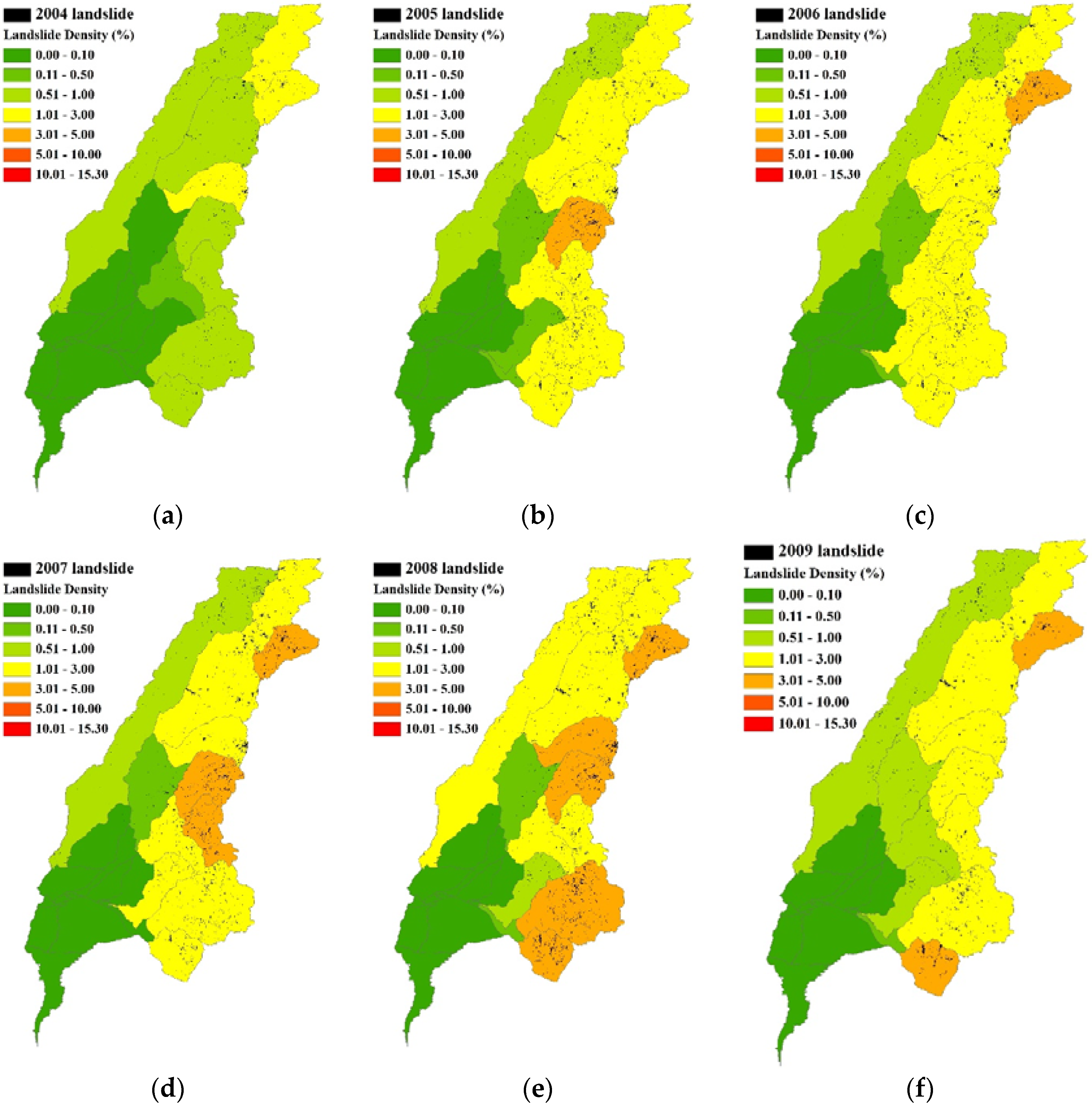
15], the advantages of this system is the larger scene coverage and much higher revisit rate, which makes Formosat-2 imagery an ideal remote sensing data source to derive high quality LC maps with less cloud and shadow contamination. Additionally, with an archive from 2004 to the present date, Formosat-2 data can permit a one-decade assessment of mass wasting at a watershed-scale. Nine annual landslide maps for the study river basin were produced from Formosat-2 images taken each year from 2004 to 2012, followed by further interpretation by an expert system to delineate non-vegetated areas [16].
With regard to the downstream water responses to upland landslides, previous studies have identified the formation of hyper-concentration flow or turbidity currents in rivers [17], the occurrence of hyperpycnal flows [18] and the associated high nephelometric turbidity in reservoirs [8]. Among these downstream responses, the increased turbidity in rivers, which has both immediate and long-term adverse impacts on the public water supply, is the most important water quality issue associated with landslides in Taiwan. Peak turbidity inflow to a water treatment plant (WTP) that exceeds 10,000 NTU for an extended period of time may result in extended down time of water treatment facilities to carry out maintenance of fouled equipment, which, in turn, results in severe water service disruptions [8,19]. The long-term adverse impacts are dependent on the duration of the high-turbidity event and the turbidity baseline, which represents the non-disturbed status for individual catchments. In general, several days or weeks, depending on the intensity of disturbance, are required for sediment particles to gradually settle down and the turbidity to be restored to a baseline level [
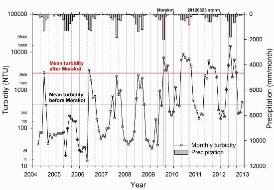
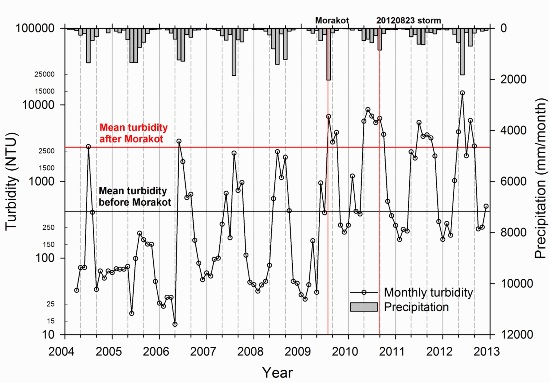
20]. However, the erosional characteristics of the Gaoping River, the largest river in Taiwan in terms of the drainage area, appear to have been fundamentally altered by the rainstorm and landslide disturbances associated with Typhoon Morakot in 2009 [21]. The following two changes occurred: (1) the probability of high-turbidity (>10,000 NTU) increased significantly after the disturbances; and (2) the turbidity has yet to return to a pre-Morakot baseline. These short- and long-term effects related to high turbidity have significantly increased the water-related stress in this area. However, the influence of landslides on these issues has rarely been examined in previous studies.
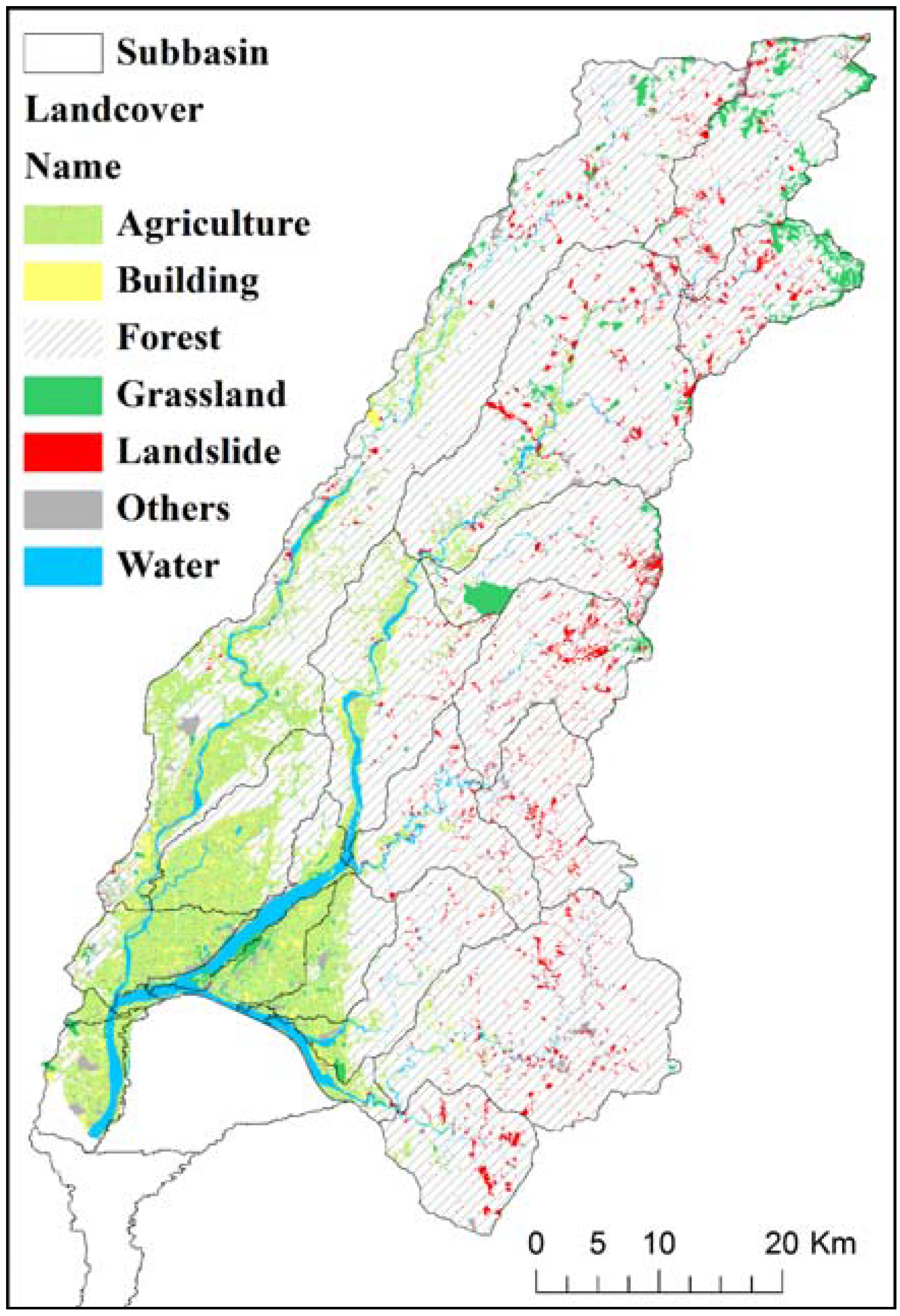
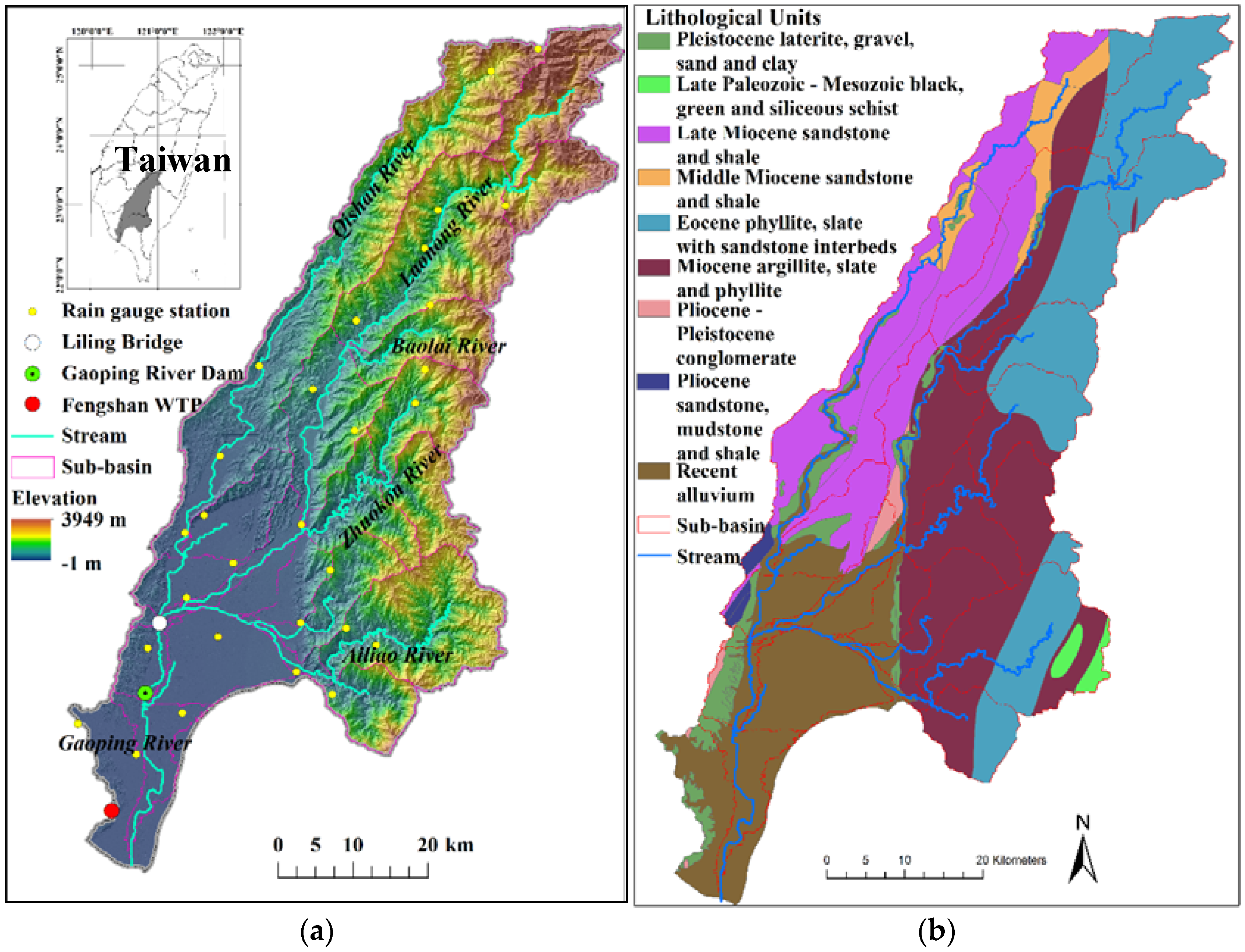
In this work, a total of nine annual land-use/land-cover (LULC) maps (2004 to 2012) of the Gaoping River Basin (GRB) were produced by overlapping each of the nine years’ Formosat-2 interpreted de-vegetative areas on the latest official LU map (2007), released by the National Land Surveying and Mapping Center (NLSC) of Taiwan. A modeling approach that integrates the LU update module of the Soil and Water Assessment Tool (SWAT) and two different types of objective functions for parameter calibration, 
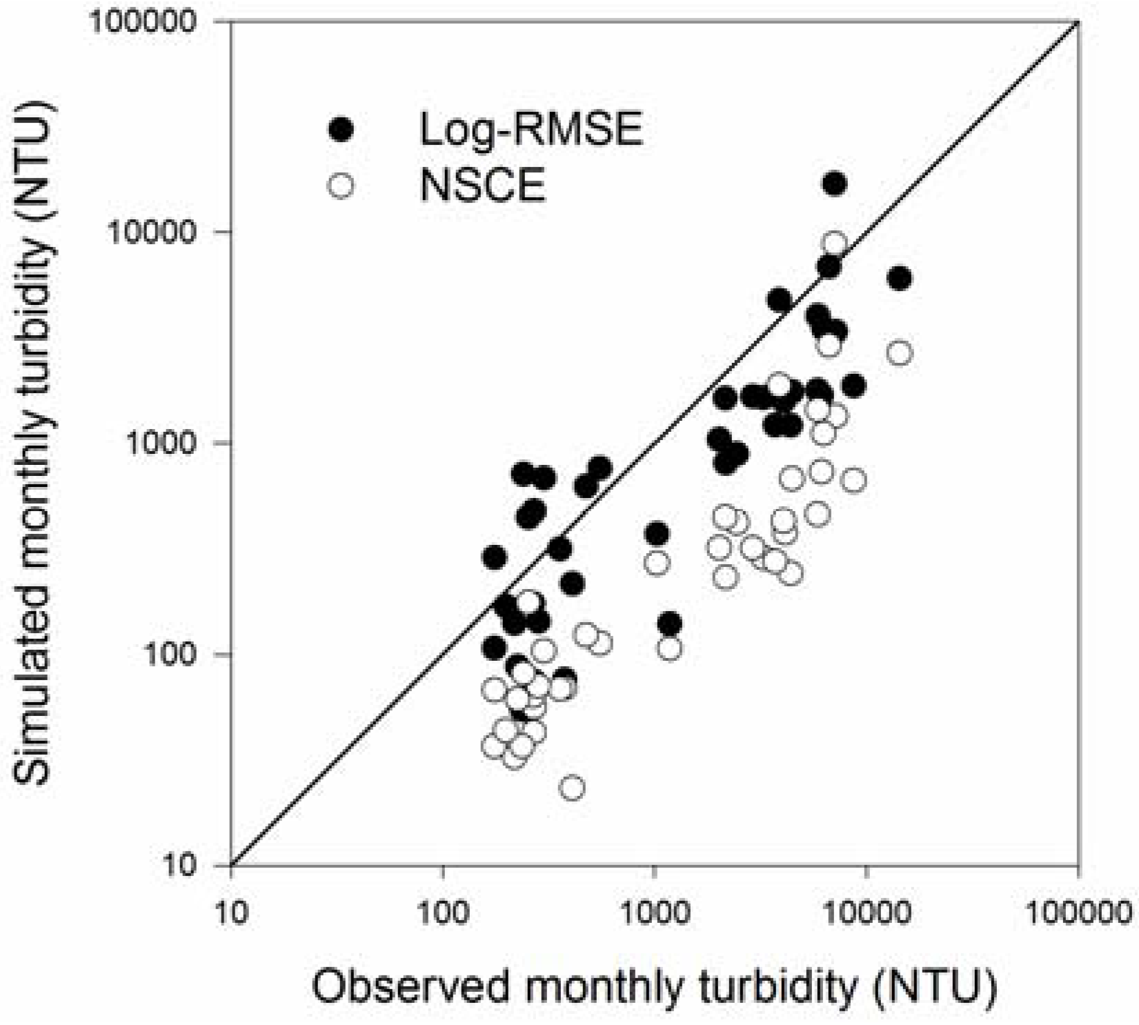
i.e., the log-scale root-mean-square-error (log-RMSE) and Nash-Sutcliffe Model Efficiency (NSCE) [22], were used to analyze the impacts of upland landslides on downstream sediment yields and turbidity. Attention was given to examining the phenomenon of the rising turbidity/sediment load baseline in the Gaoping River after Typhoon Morakot. Using these observation data and modeling results, this study discusses three main issues including: (1) the impacts of Morakot-related disturbances on downstream water quality by assessing the changes in the relationships between river flow, rainfall intensity, sediment yields and turbidity; (2) quantifying the effects of landslides on annual sediment yields by comparing the SWAT modeling with and without the land-cover updating; and (3) simulating the increased turbidity baseline by moderating the calibration strategy of SWAT.

2. Materials and Methods

2.1. Study Area

The headwaters of Gaoping River emerge from the Jade Mountain Range and flow north to south through a series of small, steep sloping basins (Figure 1a). The Gaoping River consists of five main tributaries: the Chishan, Laonong, Zhoukou, Bulao and Ailiao Rivers. While the total length (171 km) and drainage area (3257 km2) are relatively small compared to other river basins in East Asia, it has high amounts of sediment (3.6 × 10⁷ MT) and a large discharge (8.46 × 10⁹ m3) [23]. The large sediment influx is the result of high rates of erosion influenced by the frequent typhoons and a seasonal wet season (~3000 mm/year).
The nine main lithological units of the upper GRB (Figure 1b) consist of sandstone, shale and slate, while the lower basin consists of alluvium deposits. Under developed soil types dominate the mountainous to mid-elevation segments of the drainage area (Figure 1c), while alluvial soils form the bulk of the lower basin. The Liling Bridge gauging station is located at the confluence of the Qishan and Ailiao Rivers (Figure 1a) and collects hydrometric data (water discharge and suspended sediment) on the headwaters of the Gaoping River. The Gaoping River Dam (GRD) is located downstream of the gauge station (Figure 1a), supplying over 60% of the domestic water supply (about one million m3/d) for the City of Kaohsiung.
Figure 1. Geographical maps and geological settings of the Gaoping River Basin (GRB), (a) digitalized surface elevation; (b) lithological units and (c) soil types.
Water 07 06666 g001aWater 07 06666 g001b

2.2. Data Collection

2.2.1. Turbidity

Typhoon Aere and the associated landslides caused a historically high turbidity event in the Shihmen Reservoir in August 2004 resulting in a 17-day water service stoppage in Taoyuang County [24]. Thereafter, a continuous turbidity meter became an essential instrument for decision making with regard to drinking water treatment during typhoon events. During Typhoon Morakot, the maximum daily turbidity measured in GRD exceeded 40,000 NTU and remained higher than 10,000 NTU for the following 10 days resulting in a significant stoppage in water service for more than two million residents.
The Taiwan Water Corporation suggests that WTPs reduce the intake flow when the raw-water turbidity reaches 3000 NTU to prevent treatment units from being overloaded with sediment. Once a threshold of 10,000 NTU is exceeded, WTPs should completely shut down the water intake to avoid equipment breakdowns. The daily turbidity data used in this study was collected by a HACH® SS6 turbidimeter (Hach Company, Loveland, Colorado, USA) installed in the Fengshan WTP (one of the four WTPs taking raw water from GRD). Because the turbidimeter measurements are only reliable within the range from 0 to 9999 NTU, while high turbidity values (>10,000 NTU) were estimated by extrapolating the laboratory derived calibration curves of the suspended solid concentration and turbidity.

2.2.2. Precipitation

Rainfall data for SWAT modeling was input separately from 29 gauge stations in the GRB (Figure 1a). The basin average precipitation was calculated by the Thiessen polygon method (Table 1). In the period when the LC was updated (2004–2012), the average rainfall (3716 mm) was significantly higher than during the previous six years from 1998-2003 (2942 mm). The precipitation distribution (Figure 2) is typical for a tropical climate (a tropical wet and dry or savanna climate), in which more than 80% of the annual precipitation is concentrated in a five month wet season. Typhoon Morakot struck Taiwan on 7 August 2009, bringing 1900 mm of rainfall in three days.
Table 1. Summary of the annual average precipitation derived by Thiessen’s polygon method and land-use/land-cover (LULC) updating results of the Gaoping River Dam (GRD) catchment during the study period.
YearPrecipitation (mm)Land Cover Ratio (%)
ForestAgricultureGrasslandWaterBuildingLandslideOthers
19983388*
19993030
20002986
20014133
20022015
20032101
2004296070.814.52.14.73.12.52.3
2005506970.314.52.04.73.13.22.2
2006396570.214.52.04.73.13.42.1
2007411070.214.52.04.73.13.32.2
2008432570.014.52.04.63.13.52.3
2009340670.414.52.04.73.13.02.3
2010307466.214.31.44.53.18.22.3
2011255067.614.41.64.53.16.52.3
2012398967.914.41.74.53.16.22.2
Average340769.315.11.94.63.14.40.8
Note: * With decreasing population and a protected drinking water area, land cover of GRB was assumed to be constant from January 1998 to July 2004. After July 2004, a new land cover came into effect and was effective until the following July. For example, the year 2005 land cover was in effect from August 2004 to July 2005.
Figure 2. Monthly averaged precipitation of GRB during the study period (1998–2012).
Water 07 06666 g002

2.2.3. River Discharge and Suspended Sediment Load

The daily river discharge (Q) and suspended sediment data from the Liling Bridge sampling location was obtained from the hydrological yearbook published by the Water Resources Agency (WRA). Suspended sediment sampling is conducted twice per month from October to June and four times per month during typhoon season (July to September) to better approximate the highly varied suspended sediment loads (Ls). On average, 30 suspended sediment concentration (Cs) are measured annually. This dataset has been widely used in previous studies [3,5,7,25]. Kao et al. (2005) [6] investigated records collected for rivers in eastern Taiwan and pointed out the poor sensitivity of the WRA measurements because more than two-thirds of the Cs values were null in the record. Therefore, the Liling Bridge dataset had 13 records with null Cs values (all collected in 1998) removed from a total of 369 measurements from 1998 to 2012.

2.2.4. Inventory of Landslides

Rainfall-triggered landslides are one of the important causes of forest degradation in Taiwan. To evaluate forest resources, the Aerial Survey Office of the Forest Bureau produced annual landslide maps by using a semi-automatic approach that delineates landslide areas with 2 m resolution Formosat-2 imagery [26]; these maps were used in this study. The semi-automatic approach integrates an automated classification method for non-vegetated areas [16] and a manual selection procedure for identifying landslides from non-vegetative areas with the assistance of aerial photos and GIS data. Figure 3 visualizes a nine-year series of landslide inventory maps (2004–2012) derived from Formosat-2 images for the catchment upstream of the GRD. To delineate landslide areas, only the Formosat-2 imagery taken before July of each year is used, and the impacts of typhoons and storms for a given year are reflected in the inventory for the following year. Therefore, the impact of Typhoon Morakot is shown in the difference between the annual landslide inventory map of 2009 (Figure 3f) and 2010 (Figure 3g).
Figure 3. Annual landslide inventories and calculated landslide densities (total area of landslide for each sub-basin) for the catchment of GRD during (a) 2004; (b) 2005; (c) 2006; (d) 2007; (e) 2008; (f) 2009; (g) 2010; (h) 2011 and (i) 2012.
Water 07 06666 g003aWater 07 06666 g003b
Landslide activity increases in small, first and second order sub-basins after Typhoon Morakot, as shown on Figure 3g. Landslide density observations show the headwater regions have landslide activity values in the range of 10% to 15% of the total land area. Entrenched meanders along the Jhoukou, Baolia and Ailao Rivers are influenced landslide activity within the basins. The high sinuosity of the meanders focused the erosive power of flows in the active channels during Morakot [27], destabilizing the outer banks and slopes.

2.3. Landslide Updating

Land-use (LU) information describes how people utilize land and is distinct from the term land-cover (LC) that is typically collected using remote sensing tools [28]. Land-use surveys in Taiwan are routinely performed about once per decade by NLSC of the Ministry of the Interior. The most recent national survey for the study area was performed in 2007 using aerial imagery technology, auxiliary GIS data and ground surveying [29]. Three levels of detail for LU classification are defined by the NLSC, which include nine (low detail), 41 (moderate detail) and 102 (high detail) LULC types. The third level classifies landslides as one of the 102 LU types. We initialized the NLSC map by replacing the LU type of “landslide” with “forest” and then, updated the initially stated LUs with nine-year Formosat-2 landslide density data, which is comprised of the total area of landslide in a sub-catchment (Figure 3) to generate a new set of LULC maps for SWAT modelling. Except for the updated landslides, the other 101 types of LU were resampled to be six LULC classes, including agriculture, building, forest, grassland, water and others (Figure 4 2007 example). This approach assumes that any changes in LC composition during the study period are due to landslides, as interpreted from the Formosat-2 imagery. This interpretation is valid, as the GRB is a Drinking Water Source Protection Area, and most human development activities are prohibited.
The updating of a new annual LC map was scheduled on each August and was effective until the following July. For example, the 2010 landslide map represents the period from August 2009 to July 2010. Among the nine-year changes (Table 1) in the land-cover classes of GRB, landslide areas generally increased during periods of high precipitation from 2004 to 2009. A 5.2% increase in newly formed landslides is observed in 2010, which marks a sudden increase in landslide activity during Typhoon Morakot.
Figure 4. Landslide updating result of the National Land Surveying and Mapping Center (NLSC) land-use survey of the GRD catchment, 2007.
Water 07 06666 g004

2.4. SWAT

The physical processes associated with water and sediment movement in land and water phases are modeled by SWAT using a combination of computational modules including those associated with hydrology, erosion/sedimentation, land management and stream routing [30]. The combination of Formosat-2 landslide data and SWAT aims to estimate suspended sediment discharges attributed to hillslope erosion on uncovered land surfaces due to landsliding, rather than to approximate the entire erodible materials that are made available and associated with landslides. Spatial variability is limited to the sub-basin scale, as shown on Figure 3, with finer scale variability not represented by SWAT. For a detailed explanation of the theory underlying SWAT computation, please refer to Neitsch et al. (2011) [30]. Two core equations for the calculation of sediment erosion and transport in land and water phases are given below.
First, the sediment yield from each sub-basin of the watershed is computed by the Modified Universal Soil Loss Equation (MUSLE) [31] that describes soil erosion processes as follows:
s e d = 11.8 ( Q s u r f q p e a k A H R U ) 0.56 K U S L E C U S L E P U S L E L S U S L E F C F R G
where sed is the sediment yield (tons/d), Qsurf is the surface runoff depth (mm/ha), qpeak is the peak surface runoff rate (m3/s), AHRU is the area of the simulated hydrologic response unit, KUSLE is the USLE soil erodibility factor determined by the soil properties, CUSLE is the USLE cover and management factor, PUSLE is the USLE support practice factor, LSUSLE is the USLE topographic factor and FCFRG is the coarse fragment factor. Instead of using rainfall to represent the energy for detaching sediment in USLE, the MUSLE uses a runoff function (bracketed part in Equation (1)) to improve the prediction of sediment yields by canceling the use of undetermined delivery ratios in USLE and allowing the simulation to be applied on a daily basis.
Second, the simplified Bagnold stream power equation that calculates the maximum amount of sediment transported in a stream as follows:
c o n c max = S P C O N × v p k S P E X P
where concmax is the maximum sediment concentration transported by water (tons/m3), vpk is the peak channel velocity (m/s), and SPCON and SPEXP are both user-defined coefficients that require calibration for different sites.
A sensitivity analysis and auto-calibration of model parameters were accomplished using the built-in tools in ArcSWAT 2009 (a public domain software developed by Texas A&M AgriLife Research, College Station, Texas, USA) [32,33]. For the simulation of sediment yields, the seven most sensitive parameters in the processes of water and sediment routing are identified (Table 2) by the sensitivity analysis tools using the one-factor-at-a-time design and Latin Hypercube sampling method. The two user-defined coefficients of SPCON and SPEXP in Equation (2), and the PUSLE in Equation (1), are the most sensitive parameters in sediment routing processes. The Manning’s coefficient for streams (CH_N(2)) and the user-defined coefficient for the regulation of total available water released to the main channels (SURLAG), are the most sensitive parameters in the part of water routing. Increases in SURLAG and CH_N(2) will lead to lower velocities of water flow in the sub-basin surface and in the main channel [34].
Table 2. Recommended ranges and calibration results of the seven most sensitive parameters for the simulation of sediment yields in sediment and water routing processes of the Soil and Water Assessment Tool (SWAT).
Sensitivity RankingParameterProcessRecommended RangeValues Calibrated by NSCEValues Calibrated by Log-RMSEParameter Description
1SPCONSediment from channels0.0001–0.010.0020.009Linear parameter for calculating the maximum amount of sediment that can be re-entrained during channel sediment routing (Equation (2))
2PUSLESediment from landscape0–10.8460.966USLE equation support practice factor (Equation (1))
3CH_N(2)Channel flow0.025–0.150.0480.065Manning coefficient for the main channel
4CN2Surface runoff±25%±0.81%±2.54%Tuning range for the compensation of initial curve number settings at moisture condition II
5SURLAGSurface runoff0–100.6233.31Surface runoff lag coefficient
6SlopeSediment from landscape±25%±0%±0%Range for the fluctuation of initial average slope steepness (m/m)
7SPEXPSediment from channels1.0–2.01.1131.732Exponent parameter for calculating sediment re-entrained in channel sediment routing (Equation (2))
The input dataset used for the modeling of river discharge and suspended sediment load at Liling Bridge are summarized as follows: (a) DEM and Soil map of GRB (Figure 1); (b) nine-year (2004 to 2012) landslide-updated LU maps; (c) daily precipitation data from 29 gauge stations in the GRB from 1998 to 2012; and (d) daily weather data from the Kaohsiung weather station from 1998 to 2012 (Central Weather Bureau, Taiwan). Both the calibration and simulation results were evaluated by the Nash Sutcliffe Model Eficiency (NSCE) and the determination coefficient (R2).
The 15-year daily-based SWAT simulation results were processed, calibrated and validated using a monthly time step. The daily observed flow and the rating-curves synthesized Ls data in Liling Bridge are also aggregated to a monthly time series and then, divided into three time periods (1998, 1999–2003 and 2004–2012) for eliminating initial bias, parameter calibration and model validation.

2.5. Objective Functions

The built-in automatic-calibration tool of ArcSWAT2009 automatically identifies a set of model parameters that can optimize the objective function or matching function which measures the divergence (or similarity) between the model-derived and observed values given in the calibration period by using the shuffled complex evolution algorithm [32]. The objective function plays an important role in determining the solution searching direction of a multi-objective calibration approach. The most widely used objective function for the simulation of sediment yields is RMSE, which tends to fit the peak values [35]. The objective functions for the measurement of goodness-of-fit, such as the NSCE or the R2, also match the peak and higher values rather than the temporal variation patterns, especially when the overall sediment yield is contributed by several major events. On the other hand, the log-transformed objective functions, which are less used in hydrological modeling, may place more emphasis on fitting the lower observed values [36]. Therefore, two objective functions, the log-RMSE and NSCE, are applied for parameter calibration in this study. The log-RMSE and NSCE are formulated as follows:
log -RMSE = { i = 1 N [ log ( Y i d e r ) log ( Y i o b s ) ] 2 N 2 } 1 / 2 , and
NSCE = 1 i = 1 N ( Y i o b s Y i d e r ) 2 i = 1 N ( Y i o b s Y ¯ o b s ) 2
where i is the index of observed values; Y i d e r , Y o b s and Y ¯ o b s are the model derived, observed and average values of the total observed Q or Ls. Importantly, there is no difference in the weighting of the two simulation objectives (Q and Ls).

3. Results and Discussion

3.1. The Alterations in Turbidity and Sediment Regimes after Typhoon Morakot

3.1.1. Turbidity

After Typhoon Morakot, turbidity in the GRD (Figure 5) increased almost by one order of magnitude during low to dry season flow conditions and became more vulnerable to subsequent mid- to wet-flow periods. This is observed during an August 2012 rainfall (639 mm), which generated Morakot-like turbidity conditions for the GRB. Under post-Morakot conditions, the probability that the turbidity (Figure 6) exceeding 3000 and 10,000 NTU increased from 3% to 21% and 0.3% to 8%. There were 66 days where the turbidity exceeded 3000 NTU and 28 days for values over 10,000, which requires partial or completely restricting the intake at water treatment facilities.
In the past (2004–2012), a total of 16 rainfall events occurred (Table 3) during which the measured maximum daily turbidity in GRD exceeded 10,000 NTU. Among those high-turbidity events, 10 are recorded after Typhoon Morakot and only two events, Fanapi and the “20120610” storm, are defined as major rainfall events (Table 4). On the other hand, four of the five events that occurred before Morakot are defined both as major rainfall and high-turbidity events. Therefore, compared to the linear relationship between maximum daily turbidity and rainfall before Morakot (R2 = 0.95, p = 0.001) (Figure 7), the maximum 24-h rainfall was no longer the most important variable explaining the occurrence of a high turbidity event (R2 = 0.06, p = 0.46). As a result, the post-Morakot basin conditions significantly increased the susceptibility to high-turbidity, indicating that now even a relatively insignificant storm can raise the turbidity.
Figure 5. Temporal trends of the observed water turbidity (left y-axis) in GRD and the monthly averaged precipitation (right y-axis) in GRB during March 2004 to December 2012.
Water 07 06666 g005
Figure 6. Probability distributions of observed water turbidity in GRD before and after Typhoon Morakot.
Water 07 06666 g006
Table 3. Summary of the top 16 rainfall-induced high turbidity events in GRD during 2004–2012 (ranked by the maximum daily turbidity).
EventDate *Cumulative Rainfall (mm)Duration (Day)Max. 24-h Rainfall (mm)Max. Daily Turbidity (NTU)
Talim21 June 2012644735845,000
0726 storm29 July 20105691019445,000
0522 storm24 May 201013354545,000
Morakot9 August 200924897119042,400 **
0829 storm30 August 2011450520440,000
0610 storm13 June 20121366838939,000
0529 storm30 May 2010334416535,000
0719 storm19 July 2011643628632,700
Kalmaegi18 July 20081043354024,000
Fanapi21 September 2010524250123,000
0803 storm6 August 201015839818,500
Mindulle4 July 20041667657718,000
Sepat19 August 20071032636014,500
Tembin29 August 201216557814,000
0609 storm10 June 20061063939013,360
Fungwong29 July 2008525234710,000
Notes: * Date denotes the day when the maximum turbidity during the event was recorded; ** Last turbidity recorded before the monitoring equipment was torn off by the flood. The turbidity measurement was not recover until 20 August 2009.
Table 4. Summary of the rainfall characteristics, observed peak daily flow and sediment contribution ratio for the top 12 major rainfall events (ranked by the maximum 24-h rainfall) in GRB during 2004–2012.
EventDateCumulative Rainfall (mm)Duration (Day)Max. 24-h Rainfall (mm)Peak Daily Discharge (CMS)Contribution Ratio * (%)
Morakot9 August24897119015,25293
Haitang5 July15744616-47
Mindulle4 July1667657710,00780
Talim5 September6192560-20
Kalmaegi8 July10433540285048
Fanapi10 September5242501283255
Bilis6 July6974476-68
0914 storm8 September6565445507540
0609 storm6 June10639390-18
0610 storm12 June13668389649955
0813 storm7 August8369367550570
Sepat103263606364
Note: * Contribution ratio was calculated by dividing the simulated monthly Ls with the annual Ls.
Figure 7. Linear relationship between maximum daily turbidity and 24-h event rainfall for major high-turbidity events in the periods after Morakot (black points) and before Morakot (white points).
Water 07 06666 g007

3.1.2. Sediment Load

The observed sediment loads (Figure 8) show fluctuations reflecting the correlation of erosion processes and basin responses to rainfall intensity. The hydrometric measurements at Liling Bridge were suspended from November 2004 to June 2007 due to bridge reconstruction. Generally, the values of Cs and Ls at Liling Bridge were smoother during 2010 to 2011 because the relatively low (Table 1) and uniform rainfall (Figure 5). The t-test of difference in means shows that there was no significant change in the measured Q and Ls after Morakot. From 2010 to 2012, as the annual precipitation was below normal and few major rainfall events occurred (Table 4), the mean Ls was even slightly lower than that before the disturbance. As shown on Figure 8, even though the change in sediment loads was minor, the average concentration of suspended sediment was significantly higher than that before Typhoon Morakot (p = 0.014).
Figure 8. Observed suspended sediment concentrations and loads in Liling Bridge from 1999 to 2012. Measurements interrupted during October 2004 to May 2007 due to reconstruction work.
Water 07 06666 g008
The annual Ls in the Gaoping River is influenced by major rainfall events which reach a maximum 24-h rainfall of 360 mm/day or a cumulative rainfall of 1000 mm (Table 4), with examples of nine typhoons contributing 60% to 90% of the annual Ls over ten years. There were only two major events during 2010–2012, Typhoon Fanapi in 2010 (55%) and the 0610 storm in 2012 (55%). Under post-Morakot conditions, the Ls may now be distributed over various flow regimes.

3.1.3. Sediment Rating Curve

A sediment rating curve (Figure 9) was established for Ls and Q obtained for pre-, during- and post-Morakot periods. The Ls-Q relationships indicated that after the disturbances related to Typhoon Morakot even a low to medium discharge could carry high suspended sediment loads (circled in Figure 9b). Huang and Montgomery (2013) [21] investigated the altered sediment regime in southern Taiwan after Typhoon Morakot using 2010–2011 hydrometric data and indicated that the decrease in the exponent value, which is assumed to be a constant, was due to the alteration of fluvial transport characteristics, while the increased coefficient denoted an increase in the low-flow sediment load. Based on the reanalysis of rating curves developed separately by the entire and 75% low to medium discharge data, during 1999 to 2012, it is evident that the post-Morakot parameters were significantly altered (Figure 9), which is mainly due to the lack of high discharge events and a weaker linear relationship (R2 = 0.2) between Log(Q) and Log(Ls). It is still not clear if the alteration of sediment transport characteristics is significant by examining the 2010–2012 rating curve. Nonetheless, the observations of turbidity and suspended sediment concentration are strong pieces of evidence that the Morakot associated disturbances in the GRB have caused a long-term impact on downstream turbidity and increased the sediment concentration transported by low to medium discharge.
Figure 9. Suspended sediment load and flow discharge (Ls-Q) rating curves developed based on measurements in Liling Bridge, Gaoping River, during the pre-Morakot (1998–2008), Morakot (2009), and post-Morakot (2010–2012) periods. Rating curves developed based on (a) all data; and (b) 75% low to medium flow data. Anomaly values are during dry and low-flow conditions (circled values).
Water 07 06666 g009
The observed daily discharge at Liling Bridge and the rating curves developed for the three periods (Figure 9) were used to synthesize a daily Ls series for calibration and validation of the SWAT model. Additionally, based on the observed turbidity in GRD and the measured Ls at Liling Bridge, a regression equation was developed to convert the SWAT simulation results from Ls to turbidity as follows:
C t = 2.52 L s 0.610 . ( n = 186 , R 2 = 0.55 )
where Ct is the level of turbidity for GRD (NTU), and the Ls is the suspended sediment load for Liling Bridge (tons/d).

3.2. Simulation of River Flow, Sediment Loads and Turbidity Using SWAT

3.2.1. River Flow Simulation

The log-RMSE based flow simulation for the calibration and validation periods (Figure 10a,b) are similar to the results derived using the NSCE calibrated parameters (Figure 10c,d). The model performance evaluated by both R2 and NSCE (Table 5) indicates that with either the use of log-RMSE or NSCE as the objective function, the simulated monthly flow rates match well with the observed ones for the overall validation period, hence verifying the hydrological model used. However, for both calibration strategies, the performance of flow simulation decreased due to the overestimation of the baseline discharge after Morakot (Figure 10b,d).
Although the difference between the flow simulation results is not significant (p = 0.16), it is evident that from the performance indicators the log-RMSE based simulation was better than that derived by the NSCE, especially in the post-Morakot validation period. By the comparisons between the calibrated values of water routing parameters selected from the sensitivity analysis result (Table 2), we conclude that the strategy of fitting the lower observed values (log-RMSE) will tend to decrease the flow velocities, as shown in the increased CH_N(2) and SURLAG values, which gives a better flow simulation result in GRD, particularly after the disturbances related to Typhoon Morakot. Additionally, there is also a slight increase in the adjustment range of the initial CN values when the log-RMSE is applied.
Figure 10. Comparisons between the simulated and observed flow rates in the calibration leftand validation) periods. Sub-figures (a,b) are the simulated results from the log-RMSE calibrated parameters; sub-figures (c,d) are the simulated results from the NSCE calibrated parameters.
Water 07 06666 g010
Table 5. Summary of the performance indicators for the SWAT modelling of river discharge and suspended sediment load during calibration and validation periods.
Time PeriodsSimulation of River Discharge with Landslide UpdatingSimulation of Suspended Sediment Load with Landslide Updating
NSCE Based CalibrationLog-RMSE Based CalibrationNSCE Based CalibrationLog-RMSE Based Calibration
NSER2NSER2NSER2NSER2
1999–2003 (Calibration)0.7520.7680.8140.8580.8880.898−16.6140.903
2004–2008 (Pre-Morakot validation)0.8970.9130.8970.9200.6690.688−10.8390.751
2009–2012 (Post-Morakot validation)0.5030.9010.7340.9010.9370.993−0.8620.976
2004–2012 (overall validation)0.7890.8520.8550.8730.8840.909−2.8310.845

3.2.2. Sediment Load Simulation

The model predicted values from each objective function match the observed data (Figure 11), as reflected by the high R2 values for the overall validation period (R2 = 0.845 and 0.909 for log-RMSE and NSCE); however, the two objective functions lead to very different results. The strategy of fitting lower sediment yields resulted in negative NSCE values for the overall simulation (Table 5), which were mainly due to the overestimation of Ls in peak months (Figure 11a,b). On the other hand, the NSCE-based calibration balanced the simulation performance of Q and Ls, in which its performance for flow simulation was not as good as the log-RMSE, but was much better in fitting the monthly suspended sediment loads, as indicated by the high NSCE values (NSCE = 0.884) and the goodness-of-fit between the simulated and observed values (Figure 11c,d).
Figure 11. Comparisons between the simulated and observed monthly suspended sediment load in the calibration (left) and validation (right) periods. Sub-figures (a,b) are the simulated results from the log-RMSE calibrated parameters; sub-figures (c,d) are the simulated results from the NSCE calibrated parameters.
Water 07 06666 g011
Although the overall Ls modeling using the NSCE calibrated parameters is accurate in both the calibration and validation period, somehow it still underestimated the key Ls patterns regarding the increased baseline after Morakot, as shown in Figure 11d. The log-RMSE based calibration overestimated most of the peak values before Typhoon Morakot, although its predictions were in better agreement with the increased baseline (Figure 11b). The results of Ls modeling from two different objective functions confirm the aforementioned observation that a permanent change in the characteristics of sediment erosion and transport occurred after Typhoon Morakot, as reflected in the changes in the SWAT model parameters for the prediction of sediment loads.
Comparing the calibrated values of sediment routing parameters (Table 2), the two user-defined coefficients of SPCON and SPEXP explain the permanent change because the differences between the two sensitive parameters, PUSLE and Slope, are relatively minor. Based on the relationship between peak channel flow velocity (vpk) and the maximum sediment concentration transported by water (concmax) (Equation (2)), a 50% increase in SPEXP will result in a 1.8 times increase in concmax if the SPCON is not changed and the vpk is assumed to be 3 m/s. On the other hand, if SPEXP is a constant, a 50% increase in SPCON will result in a 1.5 times increase in concmax. Compared to the NSCE derived parameters (Table 2), the log-RMSE calibrated SPCON and SPEXP increased by 350% and 56%, respectively, which would theoretically result in a 8.9 times increase in concmax when the vpk is 3 m/s. These results indicate that for the simulation of the increased Ls baseline after Typhoon Morakot, the model should not only take into account the effects of landslides, which provide additional sources of sediment from the landscape (details will be given in the next section), but also the increased maximum amount of sediment re-entrained during channel sediment routing, which is due to the resuspension and channel degradation [37], or specifically, the sorting of landslide debris within the channel and its related morphology. Therefore, viewed from a modeling aspect, the increased Ls or turbidity baseline will very likely not return to the previous level even if all of the landscape disturbances (i.e., Morakot associated landslides) recover.

3.2.3. Turbidity Simulation

The log-RMSE gives better simulation results for the increased monthly turbidity (Figure 12) after Morakot in the measures of log-R2 (0.74), NSCE (0.05) and RMSE (2810 NTU). The severe rainfall and landslides associated with Typhoon Morakot significantly changed the characteristics of sediment erosion and transport, and a single set of SWAT model parameters cannot achieve a satisfactory prediction for both pre- and post-Morakot. Parameters calibrated by log-RMSE, which were identified by fitting the lower observed values in the calibration period and a larger SPCON and SPEXP, better explain the increased suspended sediment and turbidity baseline after Typhoon Morakot.
Figure 12. Comparison between model-simulated and observed monthly average turbidity in GRD by using parameters calibrated by two types of objective functions.
Water 07 06666 g012

3.3. Modeling the Effects of Landslides on Annual Sediment Yields

3.3.1. Comparison between SWAT Modeling Results with and without the Use of Landslide Updating

Except for the poor simulation of the increased baseline, the combination of landslide updating and NSCE calibrated parameters performs well in the measurement of R2 and NSCE for the overall suspended sediment load simulation (Table 5 and Figure 11). In order to quantify only the effects of landslides on annual sediment yields, another simulation using the NSCE calibrated parameters, but without the use of landslide updating (with a constant landslide ratio at 3.3%), was conducted as a reference condition for comparison, which can also represent the common approach to SWAT modeling. There is no significant change in the simulated Ls before Typhoon Morakot, when the updated landslide ratio ranges from 2.5% to 3.5%, as shown in Table 6. Landslide updating became more significant after Morakot, when the simulated annual Ls increased by 17%–10%, as the landslide ratio peaked at 8.2% in late 2009 and gradually recovered to 6.2% in 2012. Compared to the annual Ls simulated by the constant landslide ratio of 3.3%, the updating strategy resulted in a −2.3%–17.6% (−0.2–3.1 Mt/yr) increase in the simulated Ls, with a −0.5%–4.9% linearly increased landslide ratio. The modeling results indicate that a 1% increase in the landslide ratio (compared to the reference condition) leads to a 3.7% increase in the annual Ls.
Table 6. Comparison between observed, NSCE simulated (w/wo landslide updating) and log-RMSE simulated annual suspended sediment yield simulation with and without the use of landslide updating.
YearLandslide Ratio (%)Observed Ls (Mt/yr)NSCE Simulated Ls (Mt/yr)Log-RMSE Simulated Ls (Mt/yr)The Effect of LU Updating on Ls (%)Difference in Landslide Ratio * (%)
January–JulyAugust–DecemberWithout UpdatingWith UpdatingWith Updating
20042.53.27.238.478.2835.2−2.3−0.1
20053.23.4-14.6614.6562.3−0.1+0.1
20063.43.3-7.187.2030.7+0.20
20073.33.5-10.9411.0350.0+0.8+0.2
20083.53.020.5410.8810.8952.7+0.1−0.5
20093.08.227.0117.4620.5363.1+17.6+4.9
20108.26.57.534.404.9923.1+13.4+3.2
20116.56.22.502.913.2217.4+10.7+2.9
20126.24.603.613.9818.9+10.2+2.9
Note: * Difference in landslide ratio was calculated by comparing the annual updated landsldie ratio to the landslide ratio of the 2007 NLSC land-use map (constant at 3.3%).
The landslide updating approach does indeed increase the sediment load, and hence, the difference between the simulated and observed values decreased, the results still indicate that the strategy of adding the annual landslide ratio cannot compensate for the deficit between the model simulated and Morakot triggered sediment discharge. The comparison between the observed and simulated Ls in 2009 indicated there is a 6.5 Mt shortage in the observed Ls, which may be due to the sediment being supplied from other sources. The identification process used to compile the landslide inventory data delineates landslide polygons apart from landslide deposition occurring in-channel, which is not accounted for using such an updating approach.
There is no straightforward relationship between the annual landslide ratio, sediment loads and precipitation (Table 6) because the annual-scale variables may be insufficient to explain the interannual variation of sediment loads [38], and the post-Morakot sediment loads are unusually low. The WRA’s flow-dependent sampling approach underestimates the post-Morakot sediment load, which is distributed over various flow regimes. This postulation of underestimation is also supported by the significant increase in turbidity observations that are continuously monitored every 5 minutes. As a result, the Log-RMSE which performs better in the turbidity simulation may provide an improved estimation of Ls.

3.3.2. Integration of Landslide Updating and SWAT Modeling

Using the model function of SWAT cannot identify significant sediment sources within the basin. Our finding is that the integration of landslide updating can simulate more sediment load, thereby improving the model performance. Although this approach cannot compensate for the total sediment load, it indicates that other sediment delivery processes are significantly contributing as sediment sources. We postulate that increased sediment transport capacity within the channel and lateral bank erosion increase the sediment supply available for transport downstream. Future study is needed to identify these sources.
As mentioned in the previous section, we propose a postulated relationship between landslide ratio and sediment loads based on the Ls simulated by NSCE (italicized values in Table 6) and log-RMSE (highlighted values in Table 6) for the before- and post-Morakot periods, respectively. Based on this relationship (Figure 13), it is estimated that for every 1% annual increase in the landslide ratio a 2.5 Mt increase in the annual suspended sediment load will occur. This estimation is based on the landslide cover, and not on the landslide depth, which is impossible to measure from remotely sensed data.
Figure 13. Relationship between SWAT simulated annual Ls and landslide ratio of GRB during 2004–2012 (p = 0.002). Note that the Ls during the period of 2004–2009 and 2010–2012, simulated by the NSCE and log-RMSE calibrated parameters.
Water 07 06666 g013

4. Conclusions and Summary

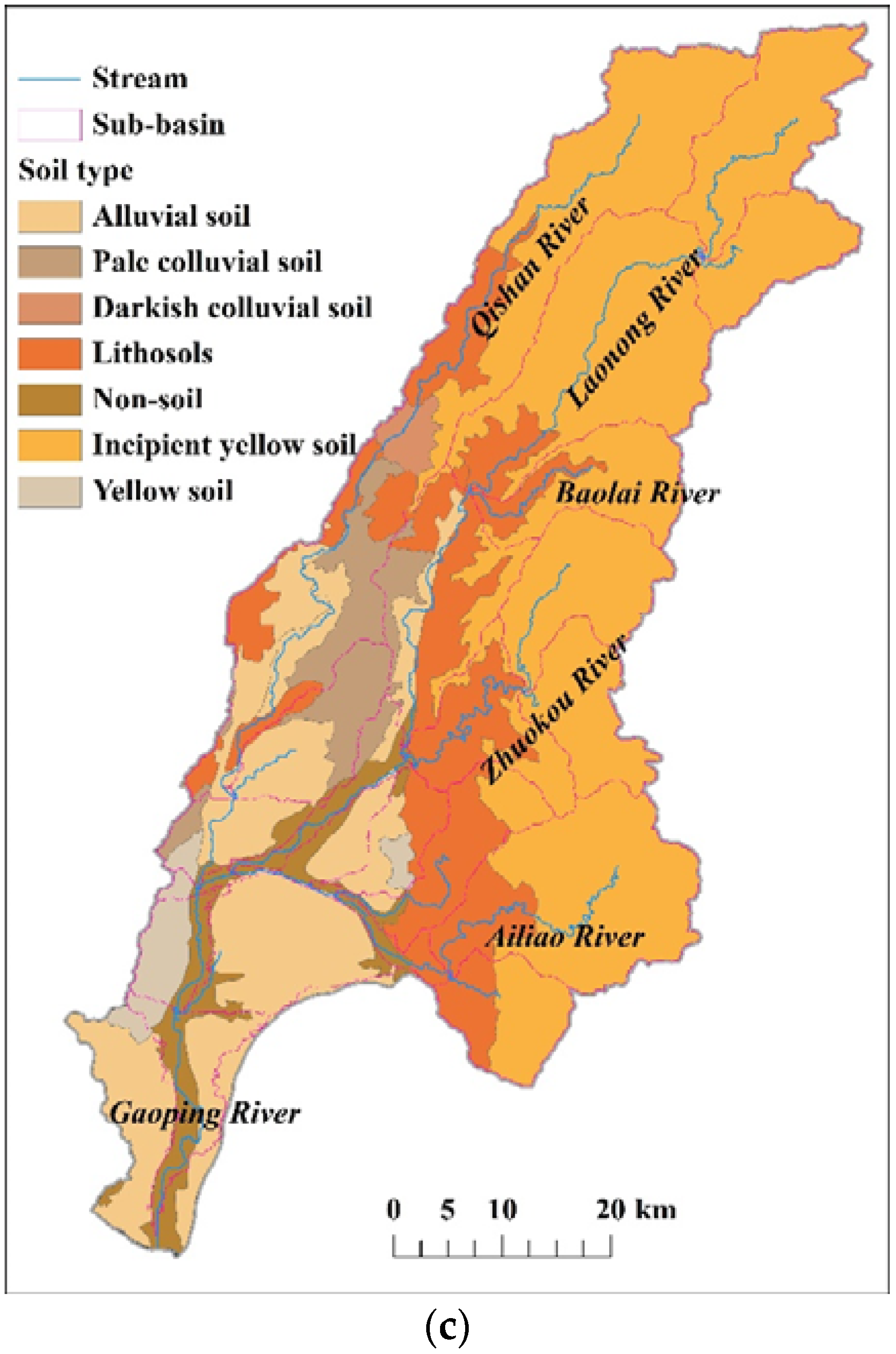
The catchment of Gaoping River is a Drinking Water Source Protection Area, where most human development activities are prohibited, and the most significant factors influencing upstream sediment erosion and transport are climatic and geomorphic processes. We determine that heavy rainfall and associated landsliding in the GRB influenced the water quality and water uses of the downstream river, particularly the level of suspended sediment and turbidity are primary concerns of the water supply.
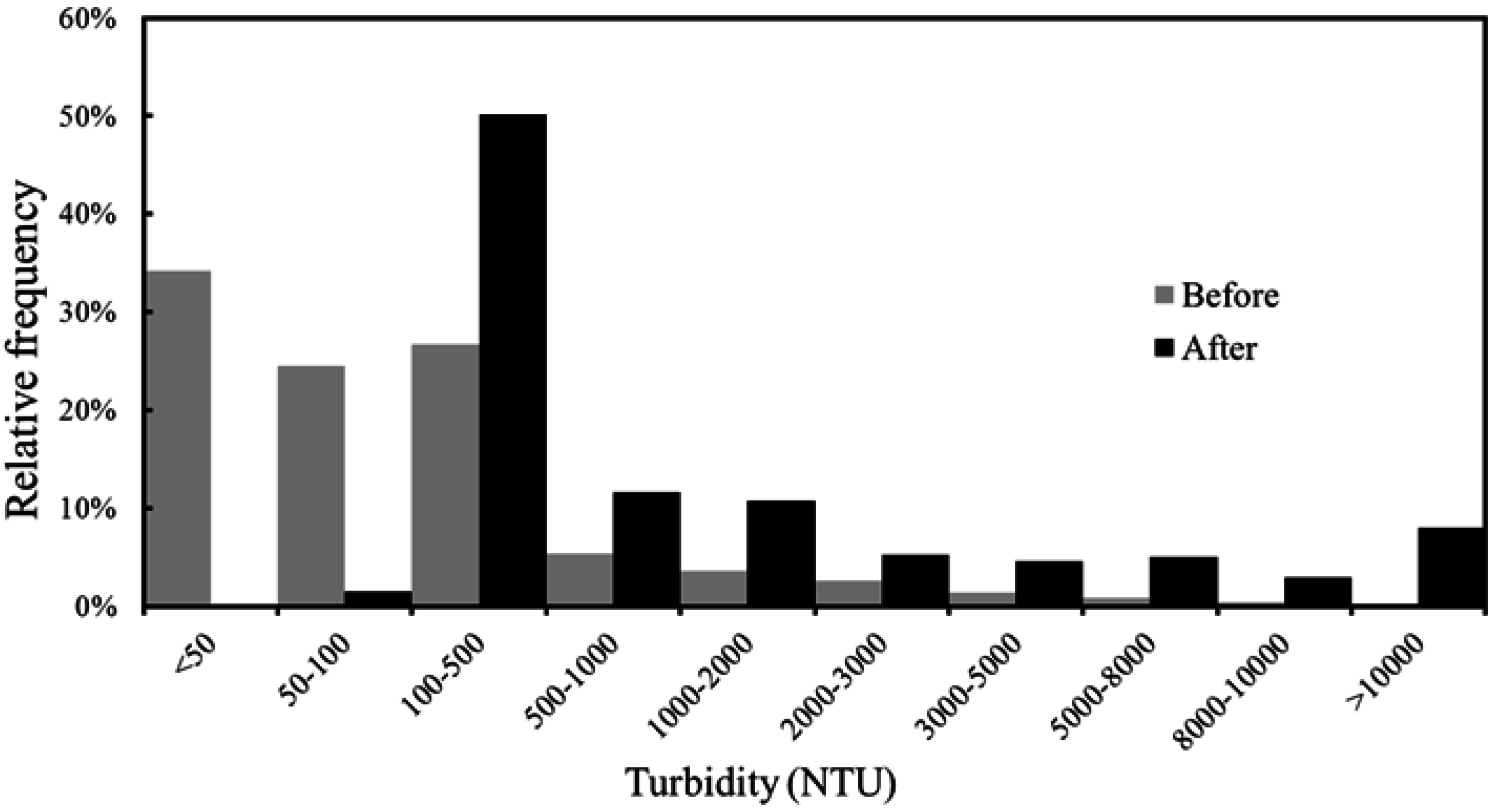
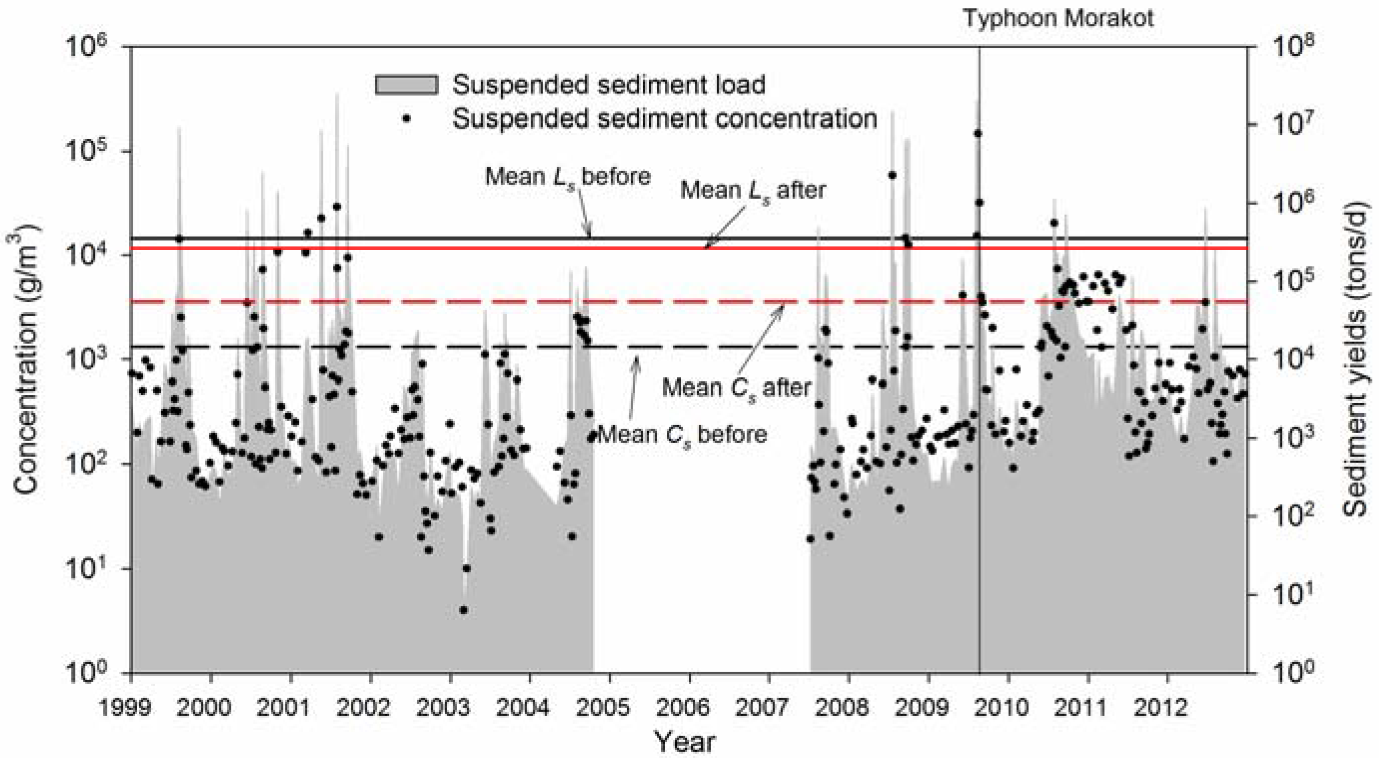
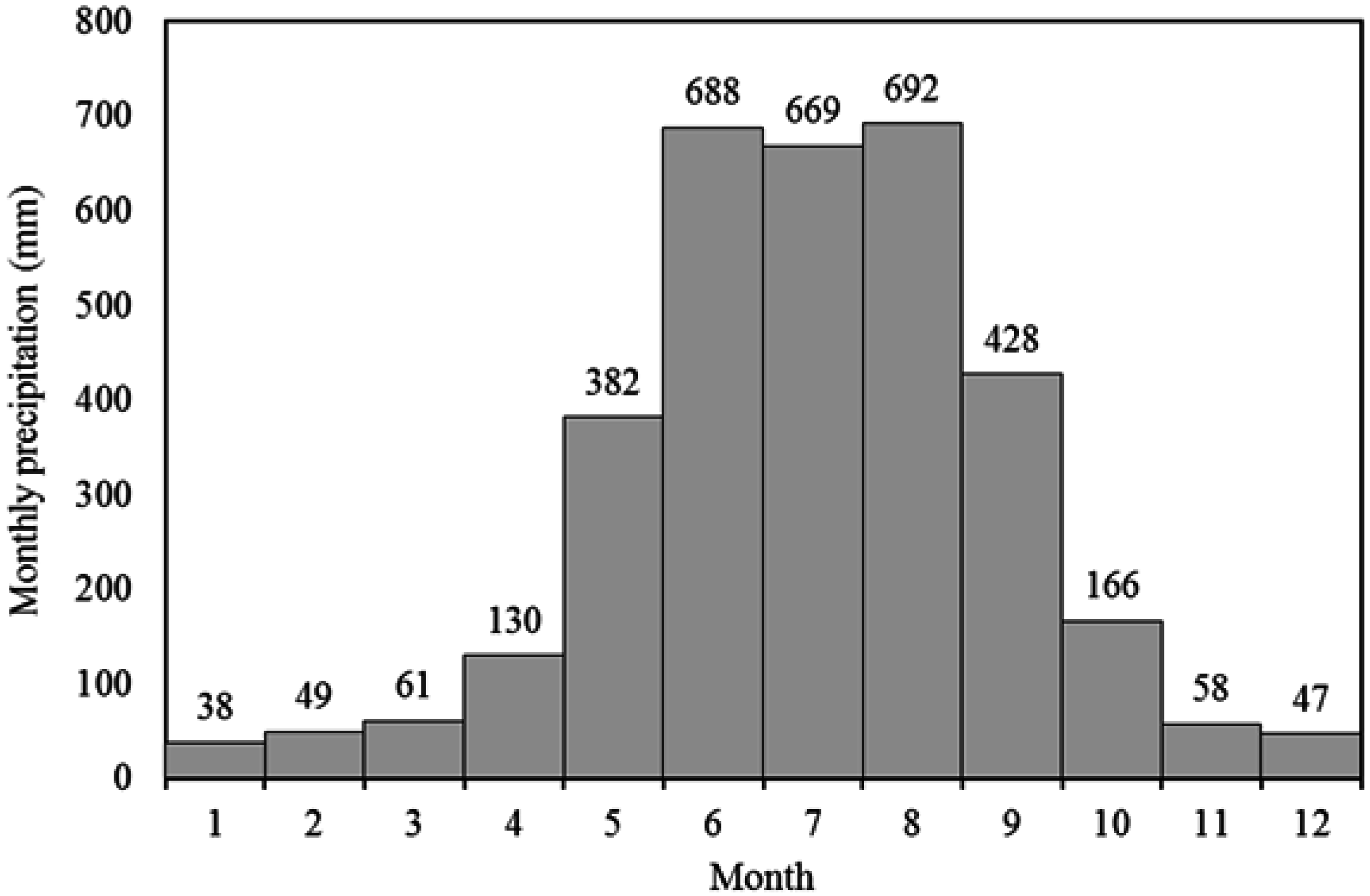
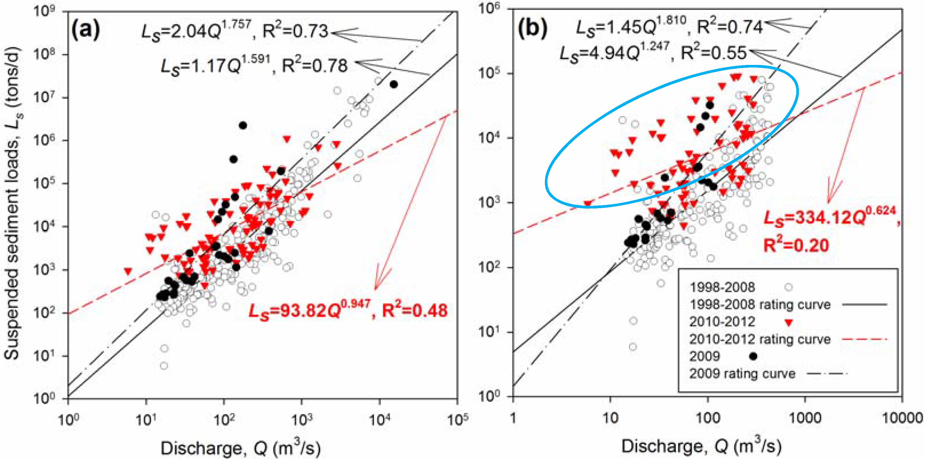
Typhoon Morakot struck the GRB on 7 August 2009, bringing 1900 mm of rainfall in three days and triggering a 5.2% increase in landslide activity. The river system responded to these disturbances with extreme sediment erosion and transport, resulting in a significant water stoppage to over two million users. After the disturbances associated with Morakot, our study found that (1) turbidity was significantly altered; (2) the correlation between event rainfall and the resulting turbidity no longer existed; and (3) the rating-curve based relationship between sediment and discharge weakened significantly after Morakot. Surprisingly, the alterations in sediment transport are non-definitive because of the low annual precipitation from 2010 to 2012.
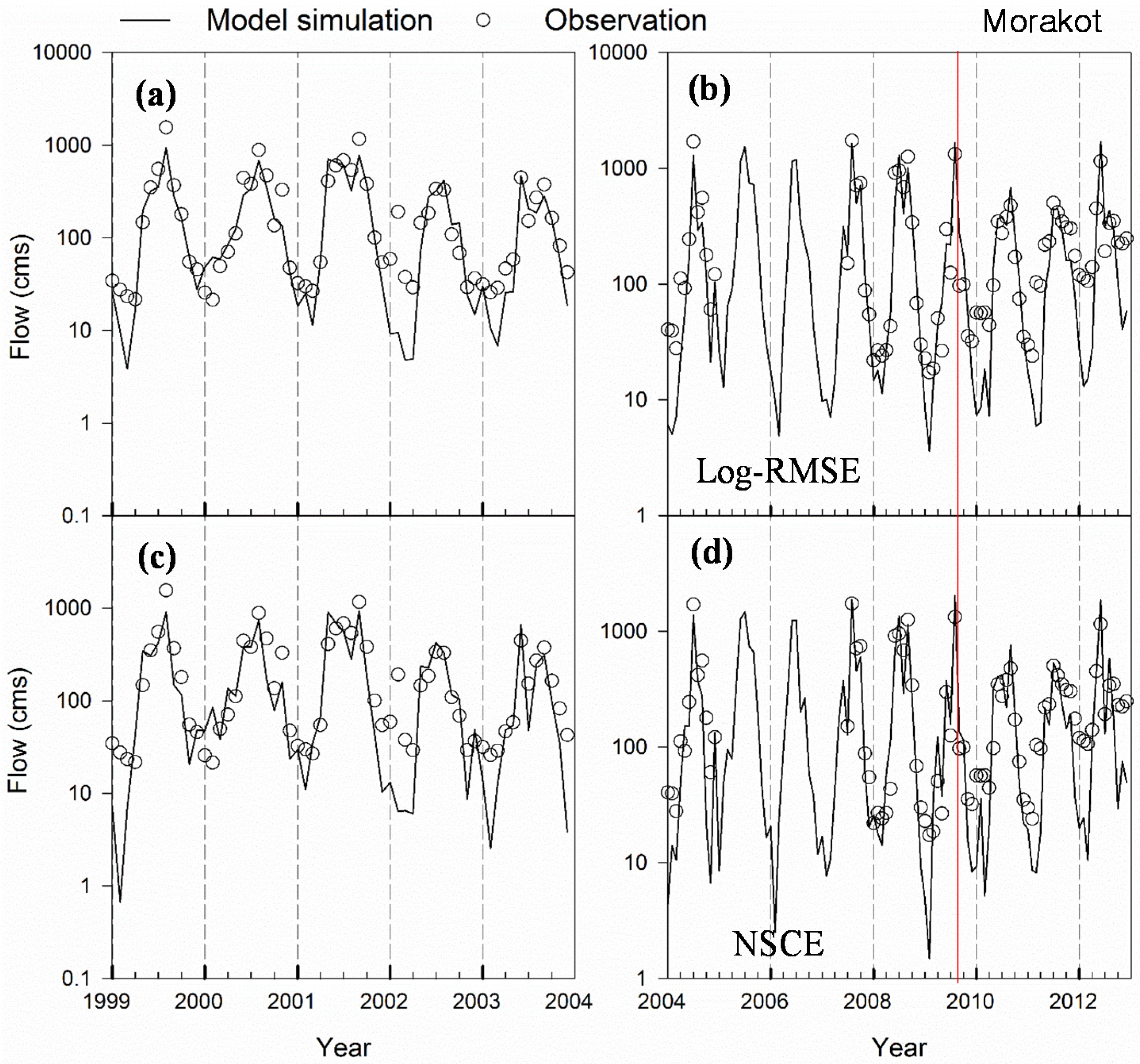
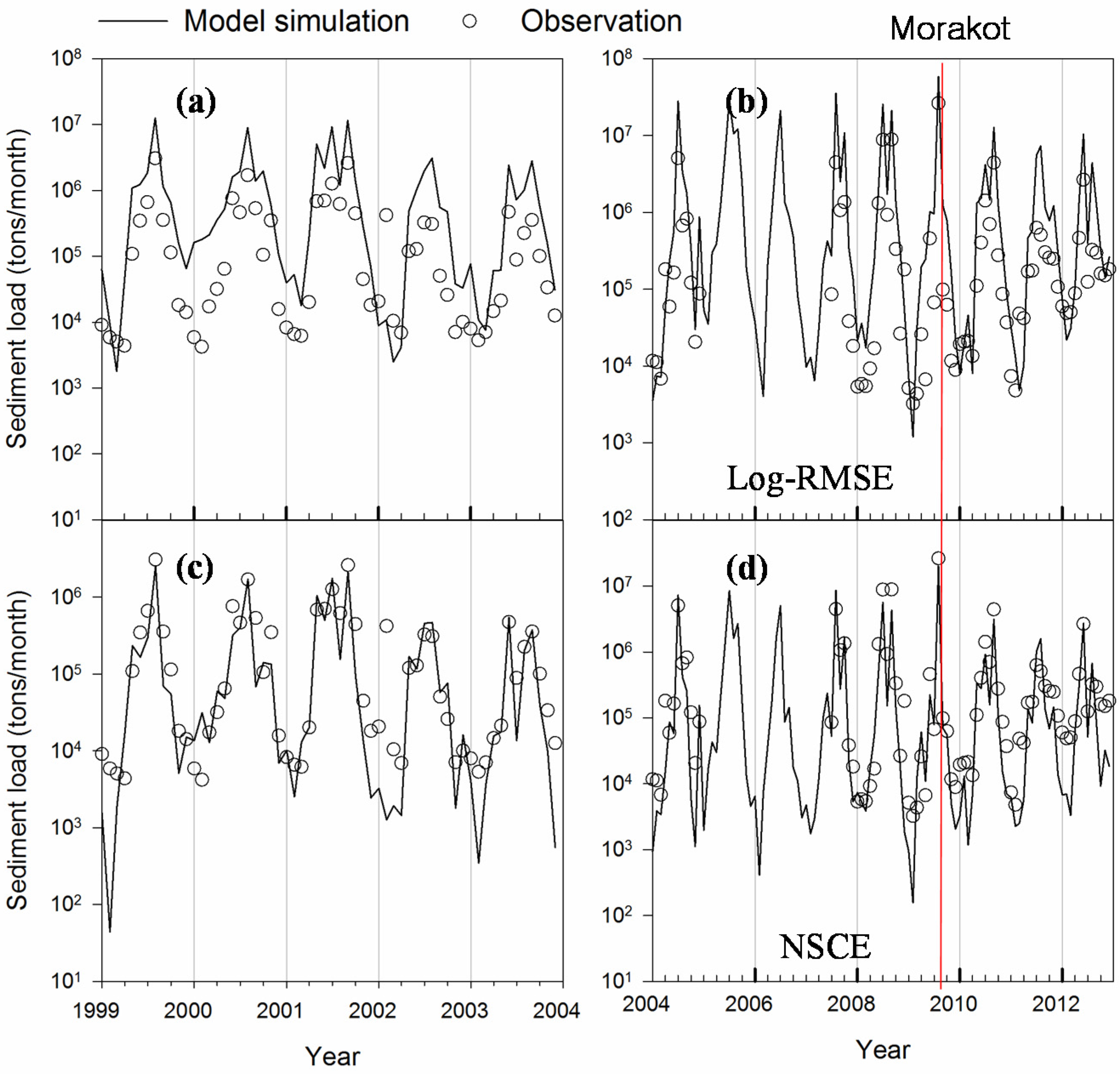
A SWAT model and two new simulation strategies were used to: (1) annually update the sub-basin with a landslide inventory map; and (2) calibrate the parameters with log-RMSE and NSCE objective functions; which used the observation data over the period 1999–2003 for the prediction of sediment load and turbidity during 2004–2012. This approach covers the river conditions before and after the typhoon induced alteration. In addition to the changed regression coefficient and exponent values of the Cs-Q rating curve that have been shown in a recent study [21], in this work a number of related changes are further revealed, as follows: the one order of the magnitude increase in turbidity baseline; the larger SPCON and SPEXP values calibrated by the log-RMSE objective function; the lower occurrence of major rainfall events but increased frequency of high-turbidity; and the poor/altered relationship between cumulative rainfall and maximum daily turbidity in major high-turbidity events.
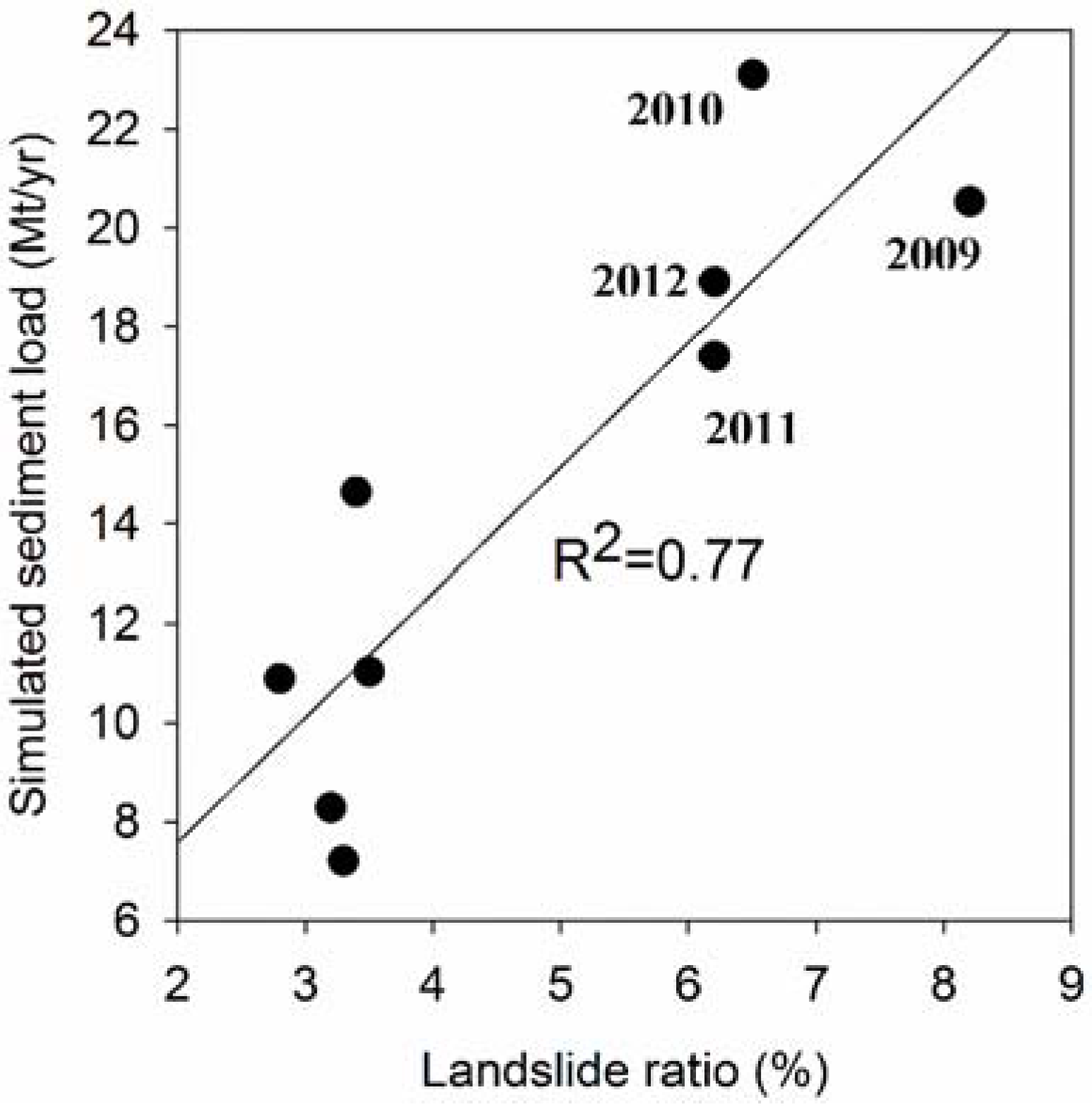
The strategy of landslide updating is carried out to improve the prediction of suspended sediment loads using a SWAT model. However, the modeling results also show that only adding the landslide ratio cannot fully address the deficit between the simulated and observed low-flow sediment discharges after Typhoon Morakot. The influence from the increased capacity of sediment that can be transported by the stream water is of significant concern. Therefore, this study recommends the use of log-RMSE calibrated parameters for the simulation of the altered suspended sediment and turbidity regime after Typhoon Morakot.
The landslide ratio decreased 2% during 2010–2012, due to the rapid growth of natural vegetation and engineered restoration methods. However, if the change in sediment transport is intrinsic, the increased turbidity baseline will likely not return to pre-Morakot levels, even after all related landslides are recovered.

Acknowledgments

The authors thank the Ministry of Science and Technology, Taiwan ROC, for the financial support through grants NSC-101-2221-E-006-153 and MOST-103-2221-E-006-014. This research was supported in part by funding received from the Headquarters of University Advancement at the National Cheng Kung University, which is sponsored by the Ministry of Education, Taiwan ROC. We thank two anonymous reviewers for their time and constructive suggestions that have improved this manuscript.

Author Contributions

Chih-Hua Chang conducted research, developed the SWAT modeling approach and wrote the initial manuscript. John Harrison contributed to data analysis, wrote the discussion, results and conclusion. Yu-Chi Huang performed data collection and ran the SWAT simulation.

Conflicts of Interest

The authors declare no conflict of interest.

References

  1. Chai, B.H.T. Structure and tectonic evolution of Taiwan. Am. J. Sci. 1972, 272, 389–422. [Google Scholar] [CrossRef]
  2. Li, Y.H. Denudation of Taiwan Island since Pliocene Epoch. Geology 1976, 4, 105–108. [Google Scholar] [CrossRef]
  3. Kao, S.J.; Milliman, J.D. Water and sediment discharge from small mountainous rivers, Taiwan: The roles of lithology, episodic events, and human activities. J. Geol. 2008, 116, 431–448. [Google Scholar] [CrossRef]
  4. Hsu, S.M.; Wen, H.Y.; Chen, N.C.; Hsu, S.Y.; Chi, S.Y. Using an integrated method to estimate watershed sediment yield during heavy rain period: A case study in Hualien County, Taiwan. Nat. Hazards Earth Syst. Sci. 2012, 12, 1949–1960. [Google Scholar] [CrossRef]
  5. Hovius, N.; Stark, C.P.; Chu, H.T.; Lin, J.C. Supply and removal of sediment in a landslide-dominated mountain belt: Central Range, Taiwan. J. Geol. 2000, 108, 73–89. [Google Scholar] [CrossRef] [PubMed]
  6. Kao, S.J.; Chan, S.C.; Kuo, C.H.; Liu, K.K. Transport-dominated sediment loading in Taiwanese rivers: A case study from the Ma-an Stream. J. Geol. 2005, 113, 217–225. [Google Scholar] [CrossRef]
  7. Dadson, S.J.; Hovius, N.; Chen, H.G.; Dade, W.B.; Hsieh, M.L.; Willett, S.D.; Hu, J.C.; Horng, M.J.; Chen, M.C.; Stark, C.P.; et al. Links between erosion, runoff variability and seismicity in the Taiwan orogen. Nature 2003, 426, 648–651. [Google Scholar] [CrossRef] [PubMed]
  8. Lin, G.-W.; Chen, H.; Petley, D.N.; Horng, M.-J.; Wu, S.-J.; Chuang, B. Impact of rainstorm-triggered landslides on high turbidity in a mountain reservoir. Eng. Geol. 2011, 117, 97–103. [Google Scholar] [CrossRef]
  9. Harris, P.T.; Hughes, M.G.; Baker, E.K.; Dalrymple, R.W.; Keene, J.B. Sediment transport in distributary channels and its export to the pro-deltaic environment in a tidally dominated delta: Fly River, Papua New Guinea. Cont. Shelf Res. 2004, 24, 2431–2454. [Google Scholar] [CrossRef]
  10. Wass, P.D.; Marks, S.D.; Finch, J.W.; Leeks, G.J.L.; Ingram, J.K. Monitoring and preliminary interpretation of in-river turbidity and remote sensed imagery for suspended sediment transport studies in the Humber catchment. Sci. Total Environ. 1997, 194, 263–283. [Google Scholar] [CrossRef]
  11. Chuang, S.C.; Chen, H.; Lin, G.-W.; Lin, C.W.; Chang, C.P. Increase in basin sediment yield from landslides in storms following major seismic disturbance. Eng. Geol. 2009, 103, 59–65. [Google Scholar] [CrossRef]
  12. Aksoy, H.; Kavvas, M.L. A review of hillslope and watershed scale erosion and sediment transport models. Catena 2005, 64, 247–271. [Google Scholar] [CrossRef]
  13. Pratt, B.; Chang, H.J. Effects of land cover, topography, and built structure on seasonal water quality at multiple spatial scales. J. Hazard. Mater. 2012, 209, 48–58. [Google Scholar] [CrossRef] [PubMed]
  14. Bathurst, J.C.; Moretti, G.; El-Hames, A.; Moaven-Hashemi, A.; Burton, A. Scenario modelling of basin-scale, shallow landslide sediment yield, Valsassina, Italian Southern Alps. Nat. Hazards Earth Syst. Sci. 2005, 5, 189–202. [Google Scholar] [CrossRef]
  15. Czaplewski, R.L. Multistage remote sensing—Toward an annual national inventory. J. For. 1999, 97, 44–48. [Google Scholar]
  16. Liu, C.-C.; Shieh, C.-L.; Lin, J.-C.; Wu, A.-M. Classification of non-vegetated areas using Formosat-2 high spatiotemporal imagery: The case of Tseng-Wen Reservoir catchment area (Taiwan). Int. J. Remote Sens. 2011, 32, 8519–8540. [Google Scholar] [CrossRef]
  17. Lin, G.-W.; Chen, H. Recurrence of hyper-concentration flows on the orogenic, subtropical island of Taiwan. J. Hydrol. 2013, 502, 139–144. [Google Scholar] [CrossRef]
  18. Dadson, S.; Hovius, N.; Pegg, S.; Dade, W.B.; Horng, M.J.; Chen, H. Hyperpycnal river flows from an active mountain belt. J. Geophys. Res. Atmos. 2005, 110. [Google Scholar] [CrossRef]
  19. Hu, C.Y.; Lo, S.L.; Chang, C.L.; Chen, F.L.; Wu, Y.D.; Ma, J.L. Treatment of highly turbid water using chitosan and aluminum salts. Sep. Purif. Technol. 2013, 104, 322–326. [Google Scholar] [CrossRef]
  20. Kobiyama, M.; Mota, A.D.A.; Grison, F.; Giglio, J.N. Landslide influence on turbidity and total solids in Cubato do Norte River, Santa Catarina, Brazil. Nat. Hazards 2011, 59, 1077–1086. [Google Scholar] [CrossRef]
  21. Huang, M.Y.F.; Montgomery, D.R. Altered regional sediment transport regime after a large typhoon, southern Taiwan. Geology 2013, 41, 1223–1226. [Google Scholar] [CrossRef]
  22. Nash, J.E.; Sutcliffe, J.V. River flow forecasting through conceptual models part I—A discussion of principles. J. Hydrol. 1970, 10, 282–290. [Google Scholar] [CrossRef]
  23. Chung, H.W.; Liu, C.C.; Chiu, Y.S.; Liu, J.T. Spatiotemporal variation of Gaoping River plume observed by Formosat-2 high resolution imagery. J. Mar. Syst. 2014, 132, 28–37. [Google Scholar] [CrossRef]
  24. Chen, C.Y.; Chen, L.K.; Yu, F.C.; Lin, S.C.; Lin, Y.C.; Lee, C.L.; Wang, Y.T. Landslides affecting sedimentary characteristics of reservoir basin. Environ. Earth Sci. 2010, 59, 1693–1702. [Google Scholar] [CrossRef] [Green Version]
  25. Dadson, S.J.; Hovius, N.; Chen, H.; Dade, W.B.; Lin, J.C.; Hsu, M.L.; Lin, C.W.; Horng, M.J.; Chen, T.C.; Milliman, J.; et al. Earthquake-triggered increase in sediment delivery from an active mountain belt. Geology 2004, 32, 733–736. [Google Scholar] [CrossRef]
  26. Taiwan Forestry Bureau (TWFB). Applying Satelliet Images in Taiwan Landslide Interpretation and Disaster Damage Analysis Project; Forest Bureau, Council of Agriculture Executive Yuan: Taipei, Taiwan, 2012. (in Chinese) [Google Scholar]
  27. Stark, C.P.; Barbour, J.R.; Hayakawa, Y.S.; Hattanji, T.; Hovius, N.; Chen, H.G.; Lin, C.W.; Horng, M.J.; Xu, K.Q.; Fukahata, Y. The climatic signature of incised river meanders. Science 2010, 327, 1497–1501. [Google Scholar] [CrossRef] [PubMed]
  28. Comber, A.; Fisher, P.; Wadsworth, R. What is land cover? Environ. Plan. B 2005, 32, 199–209. [Google Scholar] [CrossRef]
  29. Introduction to NLSC Affairs: National Land Surveying and Mapping Program. Available online: http://www.nlsc.gov.tw/En/MakePage/166?level=166 (accessed on 28 August 2015).
  30. Neitsch, S.L.; Arnold, J.G.; Kiniry, J.R.; Williams, J.R. Soil and Water Assessment Tool Theoretical Documentation Version 2009; Texas Water Resources Institute: College Station, TX, USA, 2011. [Google Scholar]
  31. Williams, J.R.; Berndt, H.D. Sediment yield prediction based on watershed hydrology. Trans. ASAE 1977, 20, 1100–1104. [Google Scholar] [CrossRef]
  32. Van Griensven, A.; Bauwens, W. Multiobjective autocalibration for semidistributed water quality models. Water Resour. Res. 2003, 39. [Google Scholar] [CrossRef]
  33. Van Griensven, A.; Meixner, T.; Grunwald, S.; Bishop, T.; Diluzio, A.; Srinivasan, R. A global sensitivity analysis tool for the parameters of multi-variable catchment models. J. Hydrol. 2006, 324, 10–23. [Google Scholar] [CrossRef]
  34. Du, J.K.; Rui, H.Y.; Zuo, T.H.; Li, Q.; Zheng, D.P.; Chen, A.L.; Xu, Y.P.; Xu, C.Y. Hydrological simulation by SWAT model with fixed and varied parameterization approaches under land use change. Water Resour. Manag. 2013, 27, 2823–2838. [Google Scholar] [CrossRef]
  35. Efstratiadis, A.; Koutsoyiannis, D. One decade of multi-objective calibration approaches in hydrological modelling: A review. Hydrol. Sci. J. 2010, 55, 58–78. [Google Scholar] [CrossRef]
  36. Bekele, E.G.; Nicklow, J.W. Multi-objective automatic calibration of SWAT using NSGA-II. J. Hydrol. 2007, 341, 165–176. [Google Scholar] [CrossRef]
  37. Arnold, J.G.; Williams, J.R.; Maidment, D.R. Continuous-time water and sediment routing model for large basins. J. Hydraul. Eng. ASCE 1995, 121, 171–183. [Google Scholar] [CrossRef]
  38. Wang, F.; Mu, X.; Hessel, R.; Zhang, W.; Ritsema, C.J.; Li, R. Runoff and Sediment load of the Yan River, China: Changes over the last 60 yr. Hydrol. Earth Syst. Sci. 2013, 17, 2515–2527. [Google Scholar] [CrossRef]

