Comparative Studies of Different Imputation Methods for Recovering Streamflow Observation

Abstract

Faulty field sensors cause unreliability in the observed data that needed to calibrate and assess hydrology models. However, it is illogical to ignore abnormal or missing values if there are limited data available. This study addressed this problem by applying data imputation to replace incorrect values and recover missing streamflow information in the dataset of the Samho gauging station at Taehwa River (TR), Korea from 2004 to 2006. Soil and Water Assessment Tool (SWAT) and two machine learning techniques, Artificial Neural Network (ANN) and Self Organizing Map (SOM), were employed to estimate streamflow using reasonable flow datasets of Samho station from 2004 to 2009. The machine learning models were generally better at capturing high flows, while SWAT was better at simulating low flows.

1. Introduction

A stream-gaging network in a watershed provides the necessary data for withdrawal uses, hydropower production, flood forecast and risk assessment, and hydrological and water quality modeling [1,2]. In addition, it is essential to have a better understanding on the spatiotemporal variations of water resources and to create effective management schemes for water resources [3]. However, streamflow records suffer from missing observations, mostly resulting from unexpected causes including records loss, sensor problems, or disruption of the data collection [2]. In the United States, Wallis et al. [4] found that at least 5% of streamflow records were missing from 1009 United States Geological Survey stream-gauges for the period from 1948 to 1988 [4]. These data would result in an incorrect response of hydrological models, but it is illogical to ignore abnormal or missing values if there is limited data available; substantial uncertainty in hydrologic and water quality modeling can be driven by these missing records.

Various data imputation methods (i.e., statistical- or physical-based methods) have been suggested to resolve missing observations [5,6,7,8]. Traditional statistical methods range from simple (e.g., listwise deletions or pairwise deletions) to advanced techniques (e.g., moving average and regression) [2]. Adopting an adequate statistical method depends on the number of missing observations, seasonal characteristics of missing observations, and available data from neighboring stations [5,9,10,11]. One drawback of statistical methods is the assumption of linearity between predictors and streamflow [10], resulting in a simplification of streamflow variation and underestimation of uncertainty. In addition, Adeloye [12] reported that regression methods could only be applicable when all predictors exist.

A physical-based model (e.g., the hydrological model) can also recover missing records when calibrated with all available data [11]. Hydrological models, however, are not only difficult to construct, but also have a site-specific limitation. Essential data for the calibration of hydrological models may be inaccessible, resulting in relative inaccuracies when calibration parameters are determined without the application of specific data from a target station [13].

Therefore, more complex nonlinear models such as artificial neural networks (ANNs) have been applied for better estimation in recovering streamflow [14,15,16]. Previous studies [9,17,18] have reported as well that the self-organizing map (SOM), an unsupervised ANN, showed satisfactory imputation results. These nonlinear models have demonstrated their performances by showing better imputation results than the traditional statistical methods [19].

For the purpose of streamflow imputation, comparison among the Soil and Water Assessment Tool (SWAT), Artificial Neural Network (ANN), and Self Organizing Map (SOM) has not been made yet. The objectives of this study were (1) to recover missing observations from the Taehwa River (TR), Korea using the Soil Water Assessment Tool model, ANN, and SOM; (2) to compare their performance in terms of streamflow imputation; and (3) to propose superior imputation methods.

2. Methods

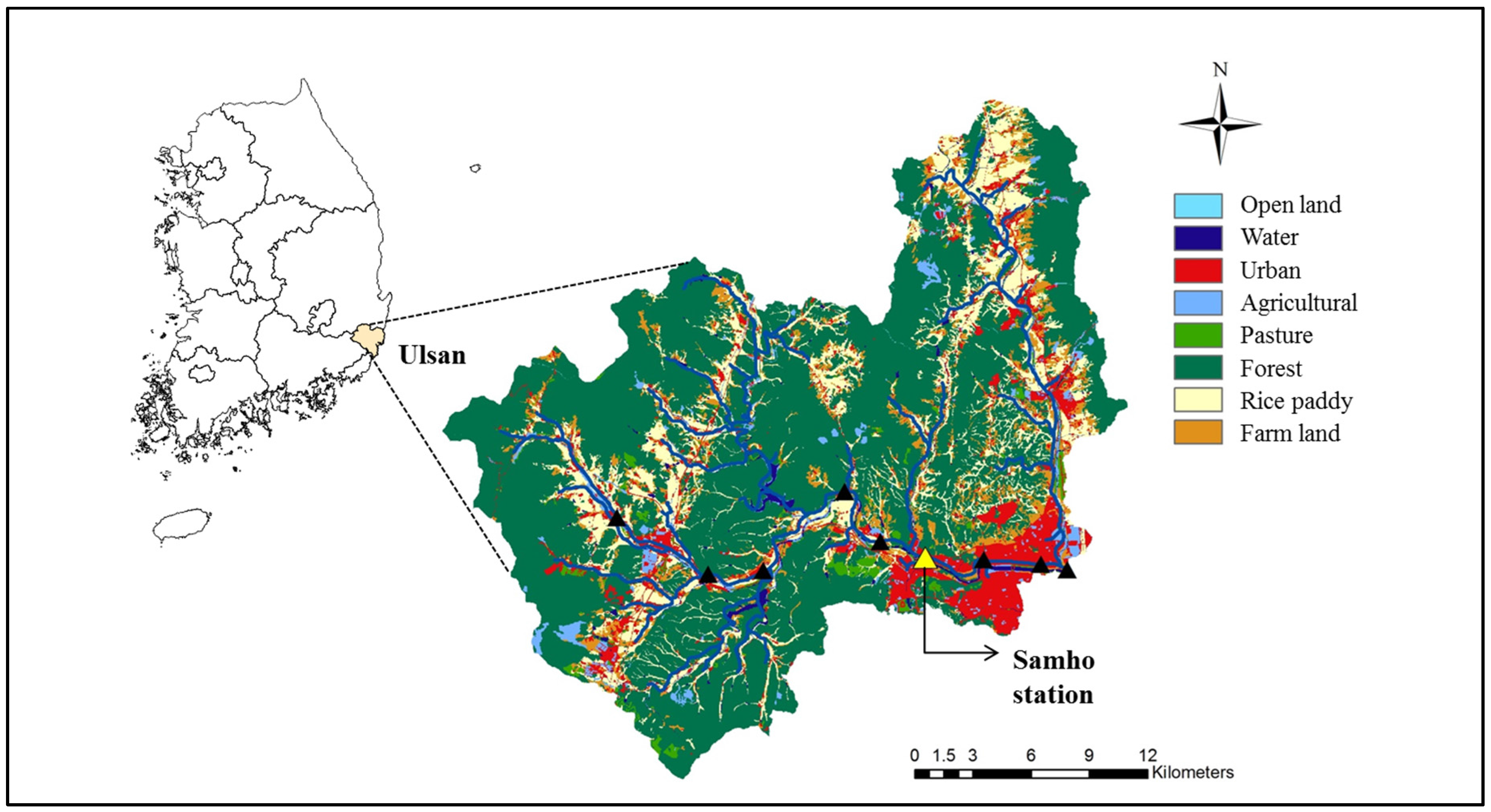
2.1. Study Area and Data Acquisition

This study explored the Taehwa River watershed, which is located in the southeastern part of Korea (129°0′ E–129°25′ E, 35°27′ N–35°45′ N). The area of the watershed is 643.96 km² and it includes most of Ulsan city and a small portion of Gyeongju city. The watershed consists of forest (62%), rice paddy (14%), and urban (10%) areas, as illustrated in Figure 1. Most of the urban areas are located downstream, while forest and rice paddies dominate the upstream. It has a moderate climate with average temperatures of 2 and 25.92 °C in January and August, respectively, and intense rainfall events during summer. The mean annual temperature of the Taehwa River watershed is 13.8 °C and the mean annual precipitation is 1274.6 mm based on the climatological normal. The TR watershed has eight flow gauging stations and Samho station, one of eight stations, is located in the middle part of the river (Figure 1). The station is not affected by tidal action.

Figure 1. Land use and location of Samho station in Taehwa River watershed.

Figure 1. Land use and location of Samho station in Taehwa River watershed.

We obtained the Digital Elevation Model (DEM), land use information, and flow rate data of Samho station from the Water Management Information System, and the soil properties from the Korean Soil information System. Weather data was obtained from Meteorological Information Portal Service System-Disaster Prevention. Additionally, we considered the discharge and water quality from Eonyang and Gulhwa Waste Water Treatment Plants (WWTPs) as point sources of Ulsan city.

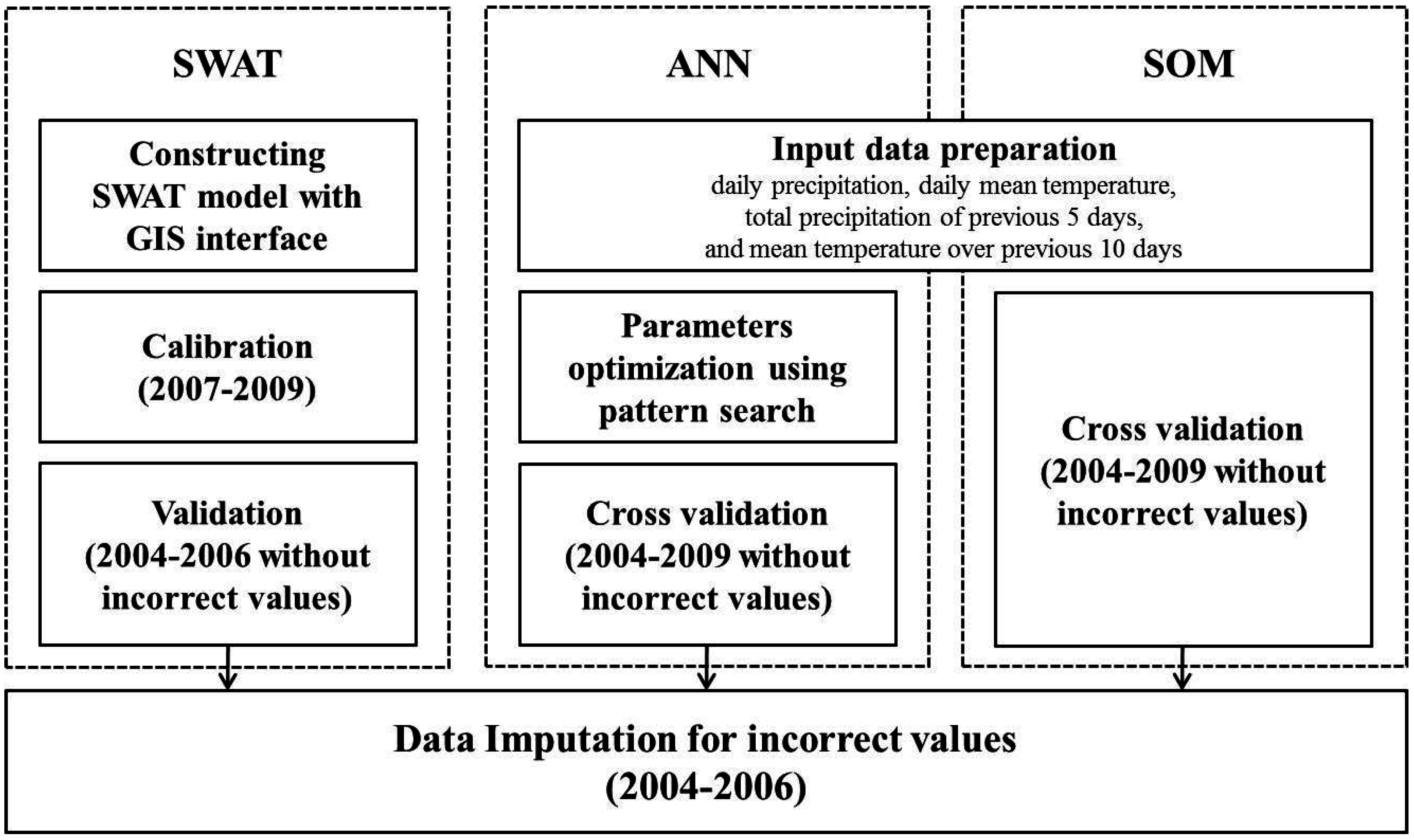
2.2. Data Imputation Methods

The Soil and Water Assessment Tool (SWAT) and two machine learning techniques, Artificial Neural Network [20] and Self Organizing Map (SOM), were applied to restore 350 flow rates in the Samho station from 2004 to 2006. The 350 flow rates had constant values caused by a faulty sensor and were regarded as missing data in this study. Figure 2 illustrates a brief framework of this study, showing calibration (2007–2009) and validation periods (2004–2006) of the SWAT model as well as the input data of the ANN and SOM models. For the ANN and SOM models, data from 2004 to 2009 were used for cross-validation.

Figure 2. Flow chart of the Data Imputation methodology of the three models: Soil and Water Assessment Tool (SWAT), Artificial Neural Network (ANN), and Self Organizing Map (SOM).

Figure 2. Flow chart of the Data Imputation methodology of the three models: Soil and Water Assessment Tool (SWAT), Artificial Neural Network (ANN), and Self Organizing Map (SOM).

2.2.1. Soil and Water Assessment Tool

SWAT is a physically distributed hydrological model developed by Jeff Arnold in the United States Department of Agriculture-Agricultural Research Service [21]. It simulates the hydrologic cycle including surface runoff, evapotranspiration, and infiltration with the consideration of water contaminations in terms of sediment, pesticides, and nutrients in a watershed. To set up the model with the Geographic Information System interface, it requires watershed characteristics including slope, land use, soil type, stream, point sources, and meteorological data including precipitation, temperature, solar intensity, relative humidity, and wind speed. SWAT divides a watershed into multiple subbasins, which consist of smaller hydrologic response units (HRU), defined by the combination of land use, slope, and soil type. The model simulates both hydrologic responses and water quality in subbasin, HRU, and reach levels by governing equations. For instance, the hydrologic process is simulated based on the water balance equation [21]:

$$S{W}_t=S{W}_0+{\displaystyle \sum }_{i=1}^t(R_{day}-Q_{surf}-E_a-w_{seep}-Q_{gw})$$

(1)

where SW_t is the final soil water content (mm H₂O), SW₀ is the initial soil water content (mm H₂O), t is the time (days), R_day is the amount of precipitation on day i (mm H₂O), Q_surf is the amount of surface runoff on day i (mm H₂O), E_a is the amount of evapotranspiration on day i (mm H₂O), w_seep is the amount of percolation and bypass flow exiting the soil profile bottom on day i (mm H₂O), and Q_gw is the amount of return flow on day i (mm H₂O).

In this study, the TR watershed was divided into 85 subbasins including 1413 HRUs. We calibrated the model using the SWAT Calibration and Uncertainty Programs (SWAT-CUP), which allows us to conduct sensitivity analysis, calibration, and parameterization [22]. This study used the SUFI-2 algorithm to calibrate 25 hydrological parameters, as tabulated in Table 1. After model calibration, we validated the model from 2004 to 2006 without the missing data.

Table 1. SWAT calibration results for 25 hydrologic parameters.

Parameter	Method	Min	Max	Rank	Value	Definition
CH_N2.rte	Replace	0.0001	0.3	1	0.0015	Manning‘s n value for the main channel length
SLSUBBSN.hru	Replace	10	150	2	18.39	Slope length (m)
CN2.mgt	Relative	−0.2	0.2	3	0.035	Moisture condition II curve number
SOL_K.sol	Relative	−0.8	0.8	4	0.19	Saturated hydraulic conductivity (mm/h)
ALPHA_BF.gw	Replace	0	1	5	0.61	Base flow recession constant
CH_K2.rte	Replace	0	150	6	77.42	Effective hydraulic conductivity of channel (mm/h)
CANMX.hru	Replace	0	15	7	0.49	Maximum canopy storage (mm H2O)
SOL_AWC.sol	Relative	−0.5	0.5	8	−0.32	Available water capacity of the soil layer (mm H2O/mm soil)
EPCO.hru	Replace	0	1	9	0.077	Plant uptake compensation factor
RCHRG_DP.gw	Replace	0	1	10	0.19	Deep aquifer percolation fraction
ESCO.hru	Replace	0	1	11	0.37	Soil evaporation compensation factor
SFTMP.bsn	Replace	0	5	12	2.55	Snowfall temperature (°C)
SURLAG.bsn	Replace	0.05	24	13	0.15	Surface runoff lag coefficient
SMFMN.bsn	Replace	0	10	14	4.85	Melt factor for snow on December 21 (mm H2O/day-°C)
TLAPS.sub	Replace	−10	10	15	−8.83	Temperature lapse rate (°C/km)
SOL_ALB.sol	Relative	0	1	16	0.58	Moist soil albedo
GWQMN.gw	Replace	0	50	17	25.95	Threshold depth of water in the shallow aquifer for return flow (mm H2O)
GW_DELAY.gw	Replace	0	100	18	94.50	Groundwater delay time (days)
TIMP.bsn	Replace	0	1	19	0.95	Snow peak temperature lag factor
REVAPMN.gw	Replace	0	500	20	324.54	Threshold depth of water in the shallow aquifer for percolation to the deep aquifer (mm H2O)
SMTMP.bsn	Replace	0	5	21	0.045	Snow melt base temperature (°C)
BIOMIX.mgt	Replace	0	1	22	0.12	Biological mixing efficiency
EPCO.bsn	Replace	0	1	23	0.55	Plant uptake compensation factor
SMFMX.bsn	Replace	0	10	24	4.91	Melt factor for snow on June 21 (mm H2O/day-°C)
ESCO.bsn	Replace	0	1	25	0.17	Soil evaporation compensation factor

Table 1. SWAT calibration results for 25 hydrologic parameters.

Parameter	Method	Min	Max	Rank	Value	Definition
CH_N2.rte	Replace	0.0001	0.3	1	0.0015	Manning‘s n value for the main channel length
SLSUBBSN.hru	Replace	10	150	2	18.39	Slope length (m)
CN2.mgt	Relative	−0.2	0.2	3	0.035	Moisture condition II curve number
SOL_K.sol	Relative	−0.8	0.8	4	0.19	Saturated hydraulic conductivity (mm/h)
ALPHA_BF.gw	Replace	0	1	5	0.61	Base flow recession constant
CH_K2.rte	Replace	0	150	6	77.42	Effective hydraulic conductivity of channel (mm/h)
CANMX.hru	Replace	0	15	7	0.49	Maximum canopy storage (mm H2O)
SOL_AWC.sol	Relative	−0.5	0.5	8	−0.32	Available water capacity of the soil layer (mm H2O/mm soil)
EPCO.hru	Replace	0	1	9	0.077	Plant uptake compensation factor
RCHRG_DP.gw	Replace	0	1	10	0.19	Deep aquifer percolation fraction
ESCO.hru	Replace	0	1	11	0.37	Soil evaporation compensation factor
SFTMP.bsn	Replace	0	5	12	2.55	Snowfall temperature (°C)
SURLAG.bsn	Replace	0.05	24	13	0.15	Surface runoff lag coefficient
SMFMN.bsn	Replace	0	10	14	4.85	Melt factor for snow on December 21 (mm H2O/day-°C)
TLAPS.sub	Replace	−10	10	15	−8.83	Temperature lapse rate (°C/km)
SOL_ALB.sol	Relative	0	1	16	0.58	Moist soil albedo
GWQMN.gw	Replace	0	50	17	25.95	Threshold depth of water in the shallow aquifer for return flow (mm H2O)
GW_DELAY.gw	Replace	0	100	18	94.50	Groundwater delay time (days)
TIMP.bsn	Replace	0	1	19	0.95	Snow peak temperature lag factor
REVAPMN.gw	Replace	0	500	20	324.54	Threshold depth of water in the shallow aquifer for percolation to the deep aquifer (mm H2O)
SMTMP.bsn	Replace	0	5	21	0.045	Snow melt base temperature (°C)
BIOMIX.mgt	Replace	0	1	22	0.12	Biological mixing efficiency
EPCO.bsn	Replace	0	1	23	0.55	Plant uptake compensation factor
SMFMX.bsn	Replace	0	10	24	4.91	Melt factor for snow on June 21 (mm H2O/day-°C)
ESCO.bsn	Replace	0	1	25	0.17	Soil evaporation compensation factor

2.2.2. Artificial Neural Network

ANN, inspired by the human brain, is a functional method for pattern classification of multi-variable datasets as well as the prediction of complex processes [23,24,25]. Many researchers have applied the ANN model to predict streamflows using input variables including rainfall, temperature, past flows, past rainfall, water levels, and so on [26,27]. For example, Bonafe et al. [28] chose the previous discharge, daily precipitation, daily mean temperature, total rainfall of the previous five days, and mean temperature over the previous ten days as input variables, and yielded a good performance in determining the daily mean flow in the upper Tiber River basin, Italy [27,28]. In this regard, ANN could be applicable for generalizing a nonlinear relationship between environmental variables and streamflows. This study selected 4 input variables to estimate daily flow, including daily precipitation, daily temperature, total precipitation of the previous 5 days, and mean temperature over the previous 10 days by reviewing the previous studies related with the data imputation of streamflows. This is because daily precipitation has a strong positive correlation with flow rate, while total precipitation of previous 5 days has a moderate positive correlation. In addition, daily mean temperature and mean temperature over previous 10 days have weak positive correlation with flow rate.

Similar to interconnected neurons in the human brain, ANN has a structure consisting of an input layer, hidden layer, output layer, and neurons (nodes) in each layer, which is connected by weights. The input layer accepts an input vector and transfers it to the network where the hidden layer determines the complexity of training, while the output layer presents the final output of the model [29,30]. Before training, weights and biases in each neuron are randomly initialized and updated by the back-propagation step [31]. In this step, signals from input vectors are transferred to the next neurons in the network where they are multiplied by weights. Finally, the transfer function in each neuron utilizes the multiplied signal as an input. This study decided to apply the Tansig function as a transfer function because it was empirically the most efficient:

$$y=f{\displaystyle \sum }_{i=1}^N{w}_i\times x_i+b$$

(2)

where $x_i$ is the input in the network, y is the output in the network, N is the number of neurons in the input vector, $w_i$ is the connection weight between input and output, f is the transfer function, and b is the bias term.

To update the weight and bias in each neuron, ANN utilizes the back-propagation algorithm where the objective function is the error between output and observation [26]. This algorithm updates weights by moving along the gradient descent of the error function, which allows the steepest decreasing change. The advantages of this algorithm are its ability to adjust the learning rate by updating the learning rate parameter and it also guarantees less oscillation with the momentum constant [32]. Equations (3) and (4) explain the back-propagation step using gradient descent with momentum algorithm:

$$\Delta w_i^{j+1}=-c\times \frac{\partial E}{\partial w_i^j}(w_i^j)+a\times \Delta w_i^j$$

(3)

$$w_i^{j+1}=w_i^j+\Delta w_i^{j+1}$$

(4)

where j is the iteration number, c is the learning rate, and a is the momentum constant.

ANN repeats the above process until the error is less than the desired goal or the number of iterations is greater than the maximum iteration. In addition, the performance of ANN models is significantly affected by parameters including number of hidden layers, number of neurons in each layer, learning rate, and momentum constant. We built the structure with one hidden layer because using one hidden layer is common in hydrologic studies [33]. For the rest of the parameters, this study employed the pattern search algorithm to find optimal parameters that maximize the model efficiency.

2.2.3. Self-Organizing Map

Kohonen was the first to propose SOM, an unsupervised machine learning technique, that clusters similar samples into a smaller dimension map while preserving the topological structure [34]. At the initial step, SOM defines the map size in an output layer by considering the number of input data. The number of map units (hexagonal lattice) is generally determined by $5\sqrt{\text{n}}$, where n represents the number of samples [35]. After setting the network size, SOM normalizes the input data and initializes weight vectors in each unit. One sample vector is randomly picked in the training step and then used to estimate the Euclidean distance with weight vectors in all the map units [36]. Then, SOM identifies the Best Matching Unit (BMU) as the map unit that has the shortest distance to the sample vector:

$$c_j=\arg mi{n}_i\{\Vert w_i-x_j\Vert \}$$

(5)

where $c_j$ is the winner unit, $x_j$ is the input vector (j = 1, 2, $\cdots$, n), $w_i$ is the weight vector (i = 1, 2, $\cdots$, m), m is the number of map units, and $\Vert \Vert$ is the distance measure, Euclidean distance.

SOM iteratively updates weight vectors of BMU and its neighboring units by using a neighborhood function to minimize the distance between them. The Gaussian distribution is applied to update the weights, as follows [34]:

$$w_i^{new}=\frac{{{\displaystyle \sum }}_{j=1}^n{h}_{c_j,i}\times x_j}{{{\displaystyle \sum }}_{j=1}^n{h}_{c_j,i}}$$

(6)

where $h_{c_j,i}$ is the neighborhood function around the winner $c_j$.

Iteration of SOM is repeated until it converges. We selected the same input variables used in the ANN model to compare the SOM performance with ANN.

2.2.4. Cross-Validation and Evaluation

Cross-validation was performed for ANN and SOM models to increase the model training efficiency. For this step, we randomly shuffled the datasets and divided them into the six subsets. Five subsets out of six were drawn for training and the remaining subset was assigned for validation. While storing the training network of the iterations, we repeated the cross validation step and selected the network with the best performance in terms of Nash–Sutcliffe efficiency coefficient (NSE). The datasets used in calibration and validation of the ANN and SOM were different because they were randomly shuffled in this step.

We evaluated model results based on the three statistics including NSE, coefficient of determination (R²), and Root Mean Square Error (RMSE). At first, NSE is a normalized statistic, indicating the fitness of a 1:1 line between observed and simulated data, and it varies from −∞ to 1. It is considered to be acceptable when values are greater than 0.5. Next, R² measures the degree of collinearity between observed and simulated data, and it varies from 0 to 1. A higher R² value means less error variance and it is considered to be acceptable when values are greater than 0.5. Last, RMSE is the error index, and a lower RMSE indicates a better model. These statistics are calculated by the equations below [37]:

$$NSE=1-\frac{{{\displaystyle \sum }}_{i=1}^n{\left(O_i-S_i\right)}^2}{{{\displaystyle \sum }}_{i=1}^n{\left(O_i-O_{avg}\right)}^2}$$

(7)

$$R^2={\left\{\frac{{{\displaystyle \sum }}_{i=1}^n\left(O_i-O_{avg}\right)\times \left(S_i-S_{avg}\right)}{{\left[{{\displaystyle \sum }}_{i=1}^n{\left(O_i-O_{avg}\right)}^2\right]}^{0.5}\times {\left[{{\displaystyle \sum }}_{i=1}^n{\left(S_i-S_{avg}\right)}^2\right]}^{0.5}}\right\}}^2$$

(8)

$$RMSE=\sqrt{\frac{1}{n}{\displaystyle \sum }_{i=1}^n{\left(O_i-S_i\right)}^2}$$

(9)

where O_i and S_i are the observed and simulated data, respectively; O_avg and S_avg are the means of the observed and simulated data, respectively; and n is the number of datum.

3. Results and Discussion

3.1. Parameter Estimation

This study calibrated 25 hydrologic parameters in SWAT as shown in Table 1, which includes the ranges of parameters, sensitivity rank, and the final values used in the calibration. CH_N2 (Manning’s n value for the main channel length) was the most sensitive parameter, followed by SLSUBBSN (Average slope length), CN2 (Moisture condition II curve number), SOL_K (Saturated hydraulic conductivity), and ALPHA_BF (Base flow recession constant). Most of the top sensitive parameters were related with channel or overland routing. This result is in agreement with previous calibration works, showing that CN2, ALPHA_BF, and SLSUBBSN were highly ranked in the sensitivity analysis [38,39,40].

Table 2 shows the ANN-associated parameters including learning rate, momentum constant, and number of neurons optimized by the pattern search method and SOM-related errors: quantization and topographic errors. The momentum constant (0.5) is less than the learning rate (0.75), implying that previous weights have more influence in updating the weights in the ANN model compared to new weights. In SOM, the quantization error measures the resolution of SOM while the topographic error does the topology preservation of SOM. The quantization (0.335) and topographic (0.039) errors in this study were within the reasonable ranges of a previous application [41].

Table 2. ANN optimized parameters and SOM related errors.

Model	Model Parameters/Error	Value
ANN (Tansig)	Learning rate	0.75
	Momentum constant	0.5
	Number of neuron	9
SOM	Quantization error	0.335
	Topographic error	0.039

Table 2. ANN optimized parameters and SOM related errors.

Model	Model Parameters/Error	Value
ANN (Tansig)	Learning rate	0.75
	Momentum constant	0.5
	Number of neuron	9
SOM	Quantization error	0.335
	Topographic error	0.039

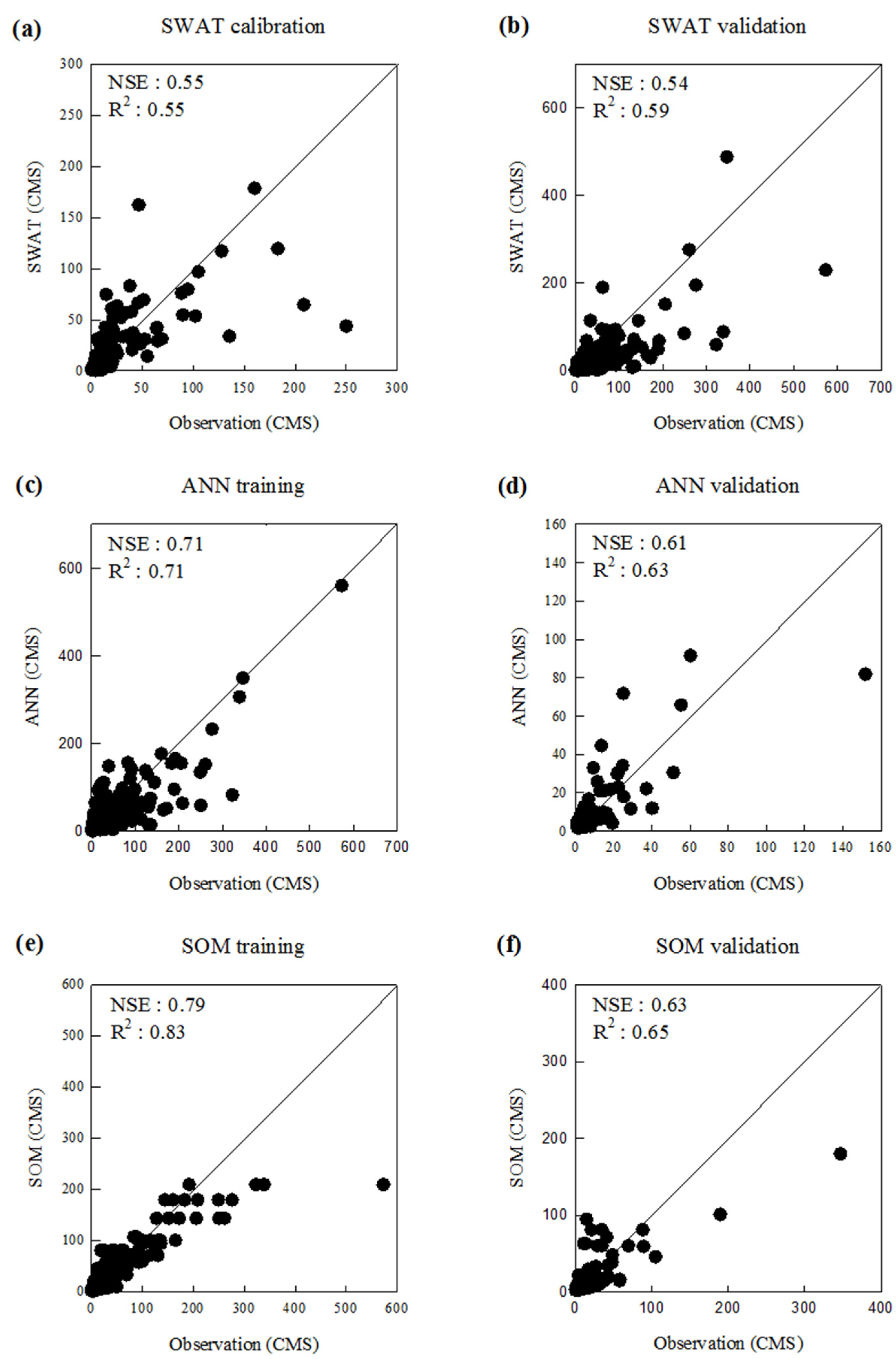
3.2. Comparison of Model Performance

The performances of SWAT, ANN, and SOM models were compared after calibration and training. Figure 3 illustrates observed and simulated flow rates in the calibration, training, and validation periods of each model, while Table 3 shows the statistical analysis with NSE and R². SWAT, ANN, and SOM had NSE values of 0.55, 0.71, and 0.79 during the calibration periods, and 0.54, 0.61, and 0.63 for the validation periods, respectively. Based on the NSE value, the three models produced acceptable results for both periods [37]. SOM showed the best performance while SWAT had the worst among them. In the case of the R², SWAT, ANN, and SOM had R² values of 0.55, 0.71, and 0.83 during the calibration periods, and 0.59, 0.63, and 0.65 for the validation periods, respectively. The values of the R² are similar with NSE or slightly greater than NSE, and SOM showed the best performance in terms of the R².

For the SWAT model, NSE values during the calibration and validation were similar. However, for the other two models the NSE values were lower in the validation period compared to the calibration period. These discrepancies were mainly due to the different datasets used in the models. SWAT had continuous time series data for both the calibration and validation periods as 2007–2009 and 2004–2006 without incorrect values, respectively. However, for the ANN and SOM, the data used for the calibration and validation periods were selected by the cross validation step. In this step, models tended to select the data with a bigger value for the calibration period to reduce the error in an efficient way. In short, the calibration period could be concentrated with the bigger value, while the rest of the data with relatively lower values went to the validation period. Therefore, NSE values were not similar during the calibration and validation for the ANN and SOM. Though NSE values were lower in the validation step for two models, they are still acceptable values.

Table 3. Calibration (training) and validation statistics for daily streamflow. NSE: Nash–Sutcliffe efficiency; R²: regression coefficient.

Method	NSE		R2
	Calibration	Validation	Calibration	Validation
SWAT	0.55	0.54	0.55	0.59
ANN	0.71	0.61	0.71	0.63
SOM	0.79	0.63	0.83	0.65

Table 3. Calibration (training) and validation statistics for daily streamflow. NSE: Nash–Sutcliffe efficiency; R²: regression coefficient.

Method	NSE		R2
	Calibration	Validation	Calibration	Validation
SWAT	0.55	0.54	0.55	0.59
ANN	0.71	0.61	0.71	0.63
SOM	0.79	0.63	0.83	0.65

Figure 3. Calibration, training, and validation results of three models: (a) SWAT calibration; (b) SWAT validation; (c) ANN training; (d) ANN validation; (e) SOM training; and (f) SOM validation.

Figure 3. Calibration, training, and validation results of three models: (a) SWAT calibration; (b) SWAT validation; (c) ANN training; (d) ANN validation; (e) SOM training; and (f) SOM validation.

Figure 4 shows the results of data imputation by the three models for 350 missing streamflows. The imputed flow rates of the ANN and SOM models showed similar trends; for example, they are both sensitive to precipitation events with comparable times and magnitudes of peaks, and the R² between them is 0.73. In contrast, SWAT generally underestimated the discharges. Based on the statistical index, SOM was considered the best model at simulating streamflow of the TR watershed. However, NSE and R² are only substantially sensitive to the high flow and they do not reflect low flow well. Hence, it is implausible to simply adopt the SOM as the best model when most of the missing streamflow was low-flow. To make a better comparison of these models, this study plotted the Flow Duration Curves (FDC) of SWAT and SOM from 2007 to 2009. ANN was excluded since it had similar trends and sensitivity to SOM.

Figure 4. Data imputation results of 350 missing flow data for the SWAT, ANN, and SOM models. Four line graphs represent the observation (red), SWAT (blue), ANN (purple), and SOM (green), while the bar graph at the top is the daily precipitation amount of the missing flow data.

Figure 4. Data imputation results of 350 missing flow data for the SWAT, ANN, and SOM models. Four line graphs represent the observation (red), SWAT (blue), ANN (purple), and SOM (green), while the bar graph at the top is the daily precipitation amount of the missing flow data.

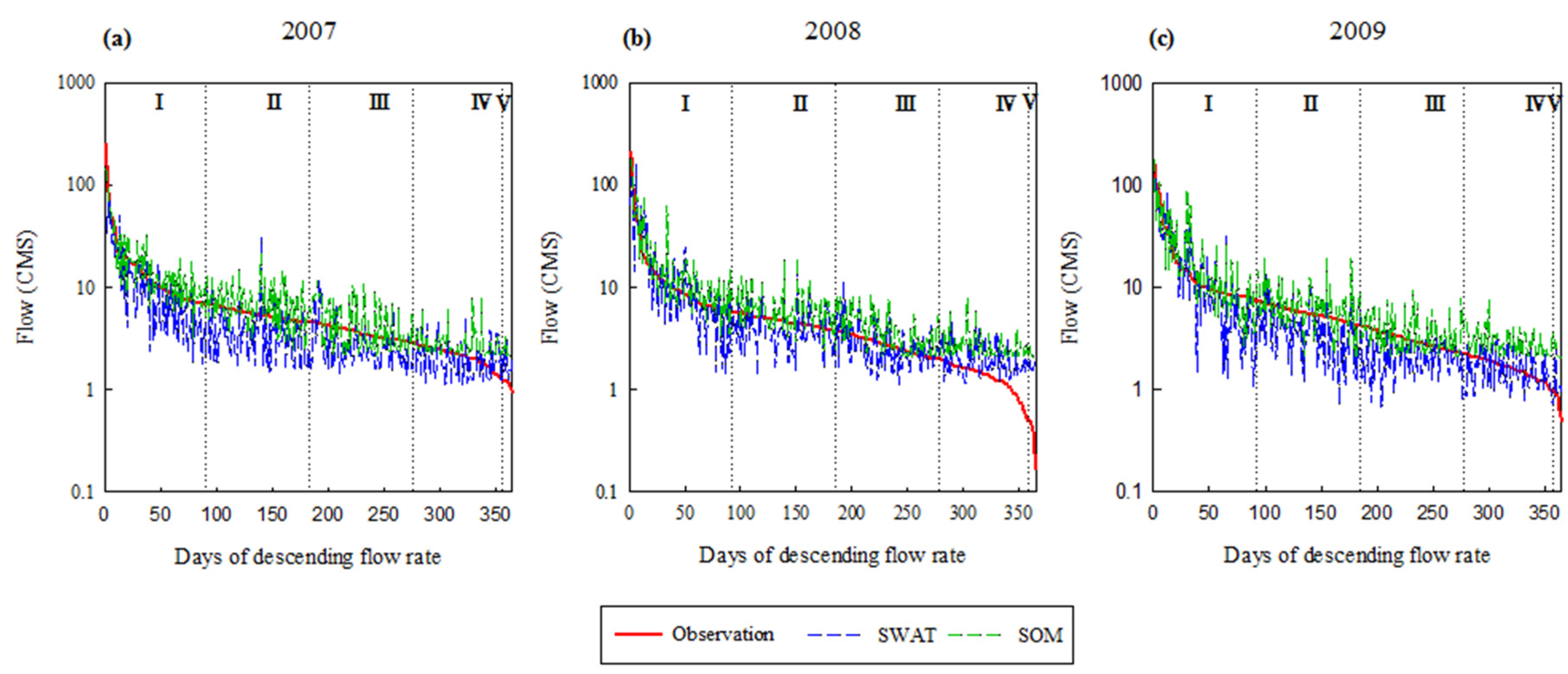
3.3. Comparison of Flow Duration Curve

Q95, Q185, Q275, and Q355 from FDC indicate the criteria for averaged-wet flow, normal flow, low flow, and drought flow, respectively [42]. This study separated FDC into five sections based on the flow indices in an attempt to compare the model performances during low-flow and high-flow separately. Figure 5 portrays the FDC of Samho station from 2007 to 2009 and shows the streamflow simulated by SWAT and SOM (dotted blue and green lines) with the observation. Table 4 shows the RMSE of SWAT and SOM in each section from 2007 to 2009. SWAT had lower RMSE than SOM for Sections II–V, which have relatively low discharges. This implies that SWAT could simulate relatively low flows better than SOM despite having smaller NSE and R² values during calibration and validation.

Figure 5. Flow duration curves (FDC) of Samho station in (a) 2007, (b) 2008, and (c) 2009. The plots are divided into five sections: I, flows over averaged-wet flow standard; II, flows between averaged-wet and normal flow standard; III, flows between normal and low flow standard; IV, flows between low and drought flow standard; and V, flows under drought flow standard.

Figure 5. Flow duration curves (FDC) of Samho station in (a) 2007, (b) 2008, and (c) 2009. The plots are divided into five sections: I, flows over averaged-wet flow standard; II, flows between averaged-wet and normal flow standard; III, flows between normal and low flow standard; IV, flows between low and drought flow standard; and V, flows under drought flow standard.

Table 4. RMSE values of SWAT and SOM in each section of FDC from 2007 to 2009.

Section	2007		2008		2009
	SWAT	SOM	SWAT	SOM	SWAT	SOM
I	24.85	12.86	22.49	11.48	3.73	4.03
II	3.76	3.81	2.33	3.38	1.66	1.91
III	1.73	2.56	1.49	2.04	1.19	1.31
IV	1	1.32	1.04	1.74	0.86	1.25
V	0.9	1.26	1.41	1.95	0.79	1.32

Better model in a section is in bold.

Table 4. RMSE values of SWAT and SOM in each section of FDC from 2007 to 2009.

Section	2007		2008		2009
	SWAT	SOM	SWAT	SOM	SWAT	SOM
I	24.85	12.86	22.49	11.48	3.73	4.03
II	3.76	3.81	2.33	3.38	1.66	1.91
III	1.73	2.56	1.49	2.04	1.19	1.31
IV	1	1.32	1.04	1.74	0.86	1.25
V	0.9	1.26	1.41	1.95	0.79	1.32

Better model in a section is in bold.

Section I, however, showed inconsistent results from 2007 to 2009. SOM has lower RMSE in 2007 and 2008, while SWAT has the lower value in 2009. This is due to the different rainfall pattern from 2007 to 2009. As shown in the blue box of Figure 6, dry and low intensity rainfall periods were found in 2009 before high intensity rainfall period. Soil moisture was low during the dry period (i.e., the blue box), thereby water infiltration throughout soil layers was enhanced and surface runoff reduced. Therefore, the magnitude of peak streamflow in 2009 was the lowest compared to 2007 and 2008 (Figure 6). In a previous work, SWAT tends to underestimate high peak flows, which is one of the limitations of the model [38,43,44,45]. This is analogous to the results in Table 5, showing that SWAT performed better in 2009 while SOM was better in 2007 and 2008. We found that the model performances in Section I substantially influenced the overall model performance as reflected in NSE or R². With the exception of 2009, wherein SWAT performed better than SOM, the machine learning technique usually shows better performance in high flow; therefore, it is recommended to use an ANN or SOM model for imputing high flow events. Otherwise, applying the SWAT model for low flow events would be more desirable. Here, the Q95 was used as a critical value to determine high flows from the whole observation. The rest of flows, which belong to Sections II–V, are considered as low flows in this study.

Figure 6. Comparison of daily performances between SWAT and SOM from 2007 to 2009 with regard to precipitation.

Figure 6. Comparison of daily performances between SWAT and SOM from 2007 to 2009 with regard to precipitation.

Table 5. R² of SWAT and SOM from 2007 to 2009.

Year	SWAT	SOM
2007	0.46	0.86
2008	0.55	0.89
2009	0.78	0.73

Better model in a section is in bold.

Table 5. R² of SWAT and SOM from 2007 to 2009.

Year	SWAT	SOM
2007	0.46	0.86
2008	0.55	0.89
2009	0.78	0.73

Better model in a section is in bold.

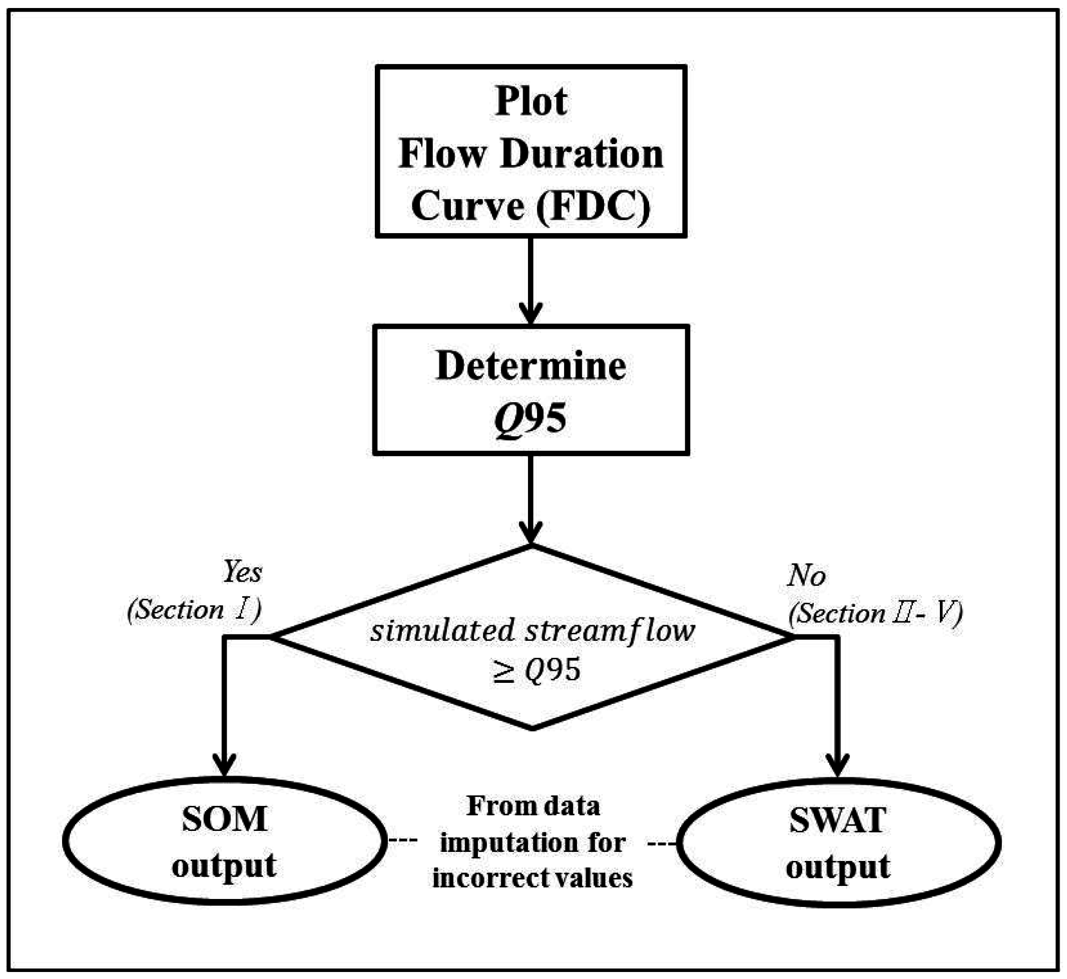
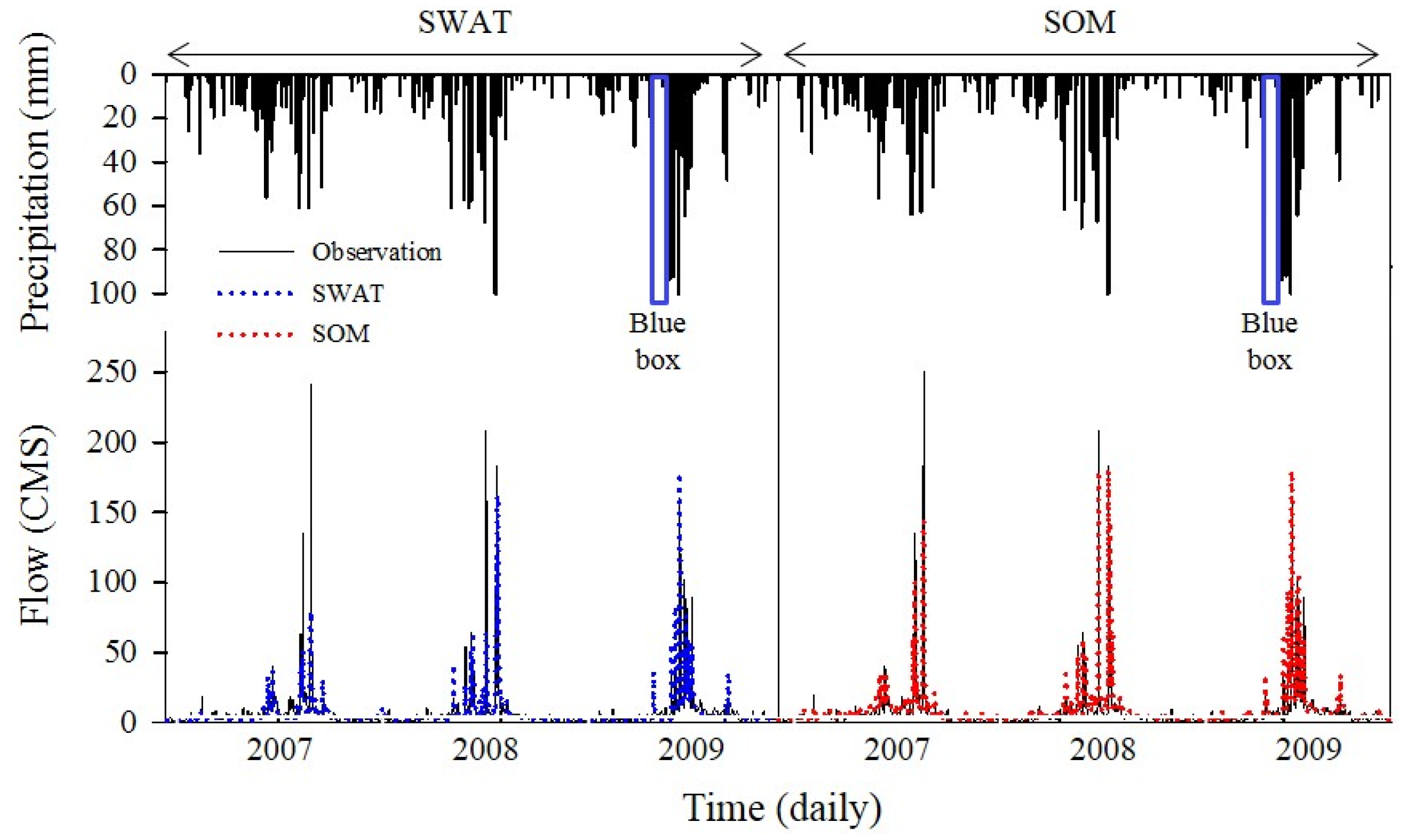
3.4. Data Imputation Result

Figure 7 summarizes the proposed data imputation algorithm using SOM and the SWAT model. The first step is to make FDC results to determine the Q95 value, which is used to separate low and high flow events. Then, it is required to first simulate the flow, using both SOM and SWAT, and compare two simulated streamflows with the Q95. If two simulated streamflows are greater than the Q95 value, the missing streamflow belongs to Section I and is substituted by the SOM output; otherwise it is categorized by Sections II–V and is substituted by the SWAT model. If two simulated streamflows belong to different sections, it is recommended to follow what SOM brings since SOM has higher accuracy of performance than SWAT.

Figure 7. The proposed data imputation algorithm using SOM and the SWAT model.

Figure 7. The proposed data imputation algorithm using SOM and the SWAT model.

In this study, we adopted the proposed data imputation algorithm to find out the best representative model output for 350 missing streamflows. We determined Q95 values from 2004 to 2006 to separate high-flow (Section I) and low-flow (Sections II–V) events; Q95 in 2004, 2005, and 2006 were 16.88, 6.99, and 10.38 cm, respectively. Two simulated streamflows were lower than the Q95 in both 2004 and 2006, while only SOM simulated streamflows were greater than Q95 in 2005. Considering the algorithm, we selected SWAT for the missing streamflows in 2004 and 2006, and SOM results were taken in 2005 for data imputation.

4. Conclusions

This study compared the performance of SWAT and two machine learning models (i.e., ANN and SOM) to recover missing streamflow in the Taehwa River watershed, Korea. Major findings from this study are as follows:

(1).

Based on the statistical index, SOM was considered the best model at simulating streamflow in the TR watershed. It demonstrated that the machine learning model is usually better at capturing high flow than SWAT.

(2).

SWAT, however, could simulate low-flows better than SOM, although it had smaller NSE and R² values.

(3).

Using an ANN or SOM model for the data imputation of high-flow events is recommended, while the SWAT model would be desirable for low-flow events.

In conclusion, using different imputation techniques according to flow characteristics is recommended and this can be explored further with different methodologies and datasets.

References

1. USGS. A New Evaluation of the Usgs Streamgaging Network; USGS: Washington, DC, USA, 1998.
2. Ng, W.W.; Panu, U.S.; Lennox, W.C. Comparative studies in problems of missing extreme daily streamflow records. J. Hydrol. Eng. 2009, 14, 91–100. [Google Scholar] [CrossRef]
3. United States Environmental Protection Agency. Clean Water Action Plan: Restoring and Protecting America’s Waters; EPA: Washington, DC, USA, 1998.
4. Wallis, J.R.; Lettenmaier, D.P.; Wood, E.F. A daily hydroclimatological data set for the continental united-states. Water Resour. Res. 1991, 27, 1657–1663. [Google Scholar] [CrossRef]
5. Gyauboakye, P.; Schultz, G.A. Filling gaps in runoff time-series in west-africa. Hydrol. Sci. J. 1994, 39, 621–636. [Google Scholar] [CrossRef]
6. Hirsch, R.M. An evaluation of some record reconstruction techniques. Water Resour. Res. 1979, 15, 1781–1790. [Google Scholar] [CrossRef]
7. Hirsch, R.M. A comparison of four streamflow record extension techniques. Water Resour. Res. 1982, 181, 1081–1088. [Google Scholar] [CrossRef]
8. Kottegoda, N.T.; Elgy, J. Infilling Missing Data, Modeling Hydrologic Processes. In Proceedings of the Fort Collings 3rd International Hydrologic Symposium on Theoretical and Applied Hydrology, Colorado State University, Fort Collins, CO, USA, 27–29 July 1977.
9. Mwale, F.D.; Adeloye, A.J.; Rustum, R. Infilling of missing rainfall and streamflow data in the shire river basin, malawi—A self organizing map approach. Phys. Chem. Earth 2012, 50, 34–43. [Google Scholar] [CrossRef]
10. Khalil, M.; Panu, U.; Lennox, W. Estimating of missing streamflows: A historical perspective. In Proceedings of the Annual Conference of the Canadian Society for Civil Engineering, Halifax, NS, Canada, 10–13 June 1998.
11. Rees, G. Hydrological data. In Manual on Low-Flow Estimation and Prediction; World Meteorological Organization: Geneva, Switzerland, 2008. [Google Scholar]
12. Adeloye, A. The relative utility of regression and artificial neural networks models for rapidly predicting the capacity of water supply reservoirs. Environ. Modell. Softw. 2009, 24, 1233–1240. [Google Scholar] [CrossRef]
13. Loke, E.A.-N.K.; Harremoes, P. Artificial Neural Networks and Grey-Box Modelling: A Comparison. In Proceedings of the Eighth International Conference: Urban Storm Drainage Proceedings, the Institution of Engineers Australisa, Sydney, Australia, 1 January 1999.
14. Ilunga, M.; Stephenson, D. Infilling streamflow data using feed-forward back-propagation (BP) artificial neural networks: Application of standard bp and pseudo mac laurin power series bp techniques. Water SA 2005, 31, 171–176. [Google Scholar]
15. Ogwueleka, T.C.; Ogwueleka, F. Feed-forward neural networks for precipitation and river level prediction. Adv. Natl. Appl. Sci. 2009, 3, 350–356. [Google Scholar]
16. Cheng, C.T.; Niu, W.J.; Feng, Z.K.; Shen, J.J.; Chau, K.W. Daily reservoir runoff forecasting method using artificial neural network based on quantum-behaved particle swarm optimization. Water 2015, 7, 4232–4246. [Google Scholar] [CrossRef]
17. Rustum, R.; Adeloye, A.J. Replacing outliers and missing values from activated sludge data using kohonen self-organizing map. J. Environ. Eng. ASCE 2007, 133, 909–916. [Google Scholar] [CrossRef]
18. Kalteh, A.M.; Hjorth, P. Imputation of missing values in a precipitation-runoff process database. Hydrol. Res. 2009, 40, 420–432. [Google Scholar] [CrossRef]
19. Dastorani, M.; Moghadamnia, A.; Piri, J.; Rico-Ramirez, M. Application of ann and anfis models for reconstructing missing flow data. Environ. Monit. Assess. 2010, 166, 421–434. [Google Scholar] [CrossRef] [PubMed]
20. Carpenter, J. Personal Communication, Occoquan Watershed Monitoring Laboratory, Department of Civil and Environmental Engineering; Virginia Tech: Manassas, VA, USA, 1999. [Google Scholar]
21. Arnold, J.G.; Srinivasan, R.; Muttiah, R.S.; Williams, J.R. Large area hydrologic modeling and assessment-part 1: Model development. J. Am. Water Resour. Assoc. 1998, 34, 73–89. [Google Scholar] [CrossRef]
22. Abbaspour, K.C. User manual for swat-cup, swat calibration and uncertainty analysis programs. In Swiss Federal Institute of Aquatic Science and Technology; Eawag: Duebendorf, Switzerland, 2007. [Google Scholar]
23. McCulloch, W.S.; Pitts, W. A logical calculus of the ideas immanent in nervous activity. Bull. Math. Biophys. 1943, 5, 115–133. [Google Scholar] [CrossRef]
24. Cho, K.H.; Sthiannopkao, S.; Pachepsky, Y.A.; Kim, K.W.; Kim, J.H. Prediction of contamination potential of groundwater arsenic in Cambodia, Laos, and Thailand using artificial neural network. Water Res. 2011, 45, 5535–5544. [Google Scholar] [CrossRef] [PubMed]
25. Guo, H.; Jeong, K.; Lim, J.; Jo, J.; Kim, Y.M.; Park, J.P.; Kim, J.H.; Cho, K.H. Prediction of effluent concentration in a wastewater treatment plant using machine learning models. J. Environ. Sci. 2015, 32, 90–101. [Google Scholar] [CrossRef] [PubMed]
26. Govindaraju, R.S. Artificial neural networks in hydrology. I: Preliminary concepts. J. Hydrol. Eng. 2000, 5, 115–123. [Google Scholar]
27. Govindaraju, R.S. Artificial neural networks in hydrology. II: Hydrologic applications. J. Hydrol. Eng. 2000, 5, 124–137. [Google Scholar]
28. Bonafe, A.; Galeati, G.; Sforna, M. Neural networks for daily mean flow forecasting. Hydraul. Eng. Softw. V 1994, 1, 131–138. [Google Scholar]
29. Dawson, C.W.; Wilby, R. An artificial neural network approach to rainfall-runoff modelling. Hydrol. Sci. J. 1998, 43, 47–66. [Google Scholar] [CrossRef]
30. Wang, Y.; Guo, S.L.; Xiong, L.H.; Liu, P.; Liu, D.D. Daily runoff forecasting model based on ANN and data preprocessing techniques. Water 2015, 7, 4144–4160. [Google Scholar] [CrossRef]
31. Shukla, M.B.; Kok, R.; Prasher, S.O.; Clark, G.; Lacroix, R. Use of artificial neural networks in transient drainage design. Trans. ASAE 1996, 39, 119–124. [Google Scholar] [CrossRef]
32. Rojas, R. Neural Networks: A Systematic Introduction; Springer: Berlin, Germany, 1996. [Google Scholar]
33. Dawson, C.W.; Wilby, R.L. Hydrological modelling using artificial neural networks. Progress Phys. Geogr. 2001, 25, 80–108. [Google Scholar] [CrossRef]
34. Kalteh, A.M.; Hiorth, P.; Bemdtsson, R. Review of the self-organizing map (SOM) approach in water resources: Analysis, modelling and application. Environ. Modell. Softw. 2008, 23, 835–845. [Google Scholar] [CrossRef]
35. Vesanto, J. Neural Network Tool for Data Mining: Som Toolbox. In Proceedings of the Symposium on Tool Environments and Development Methods for Intelligent Systems (TOOLMET2000), Oulu, Finland, 13–14 April 2000.
36. Huang, R.Q.; Xi, L.F.; Li, X.L.; Liu, C.R.; Qiu, H.; Lee, J. Residual life predictions for ball bearings based on self-organizing map and back propagation neural network methods. Mech. Syst. Signal Proc. 2007, 21, 193–207. [Google Scholar] [CrossRef]
37. Moriasi, D.N.; Arnold, J.G.; van Liew, M.W.; Bingner, R.L.; Harmel, R.D.; Veith, T.L. Model evaluation guidelines for systematic quantification of accuracy in watershed simulations. Trans. Asabe 2007, 50, 885–900. [Google Scholar] [CrossRef]
38. Cho, K.H.; Pachepsky, Y.A.; Kim, J.H.; Kim, J.W.; Park, M.H. The modified swat model for predicting fecal coliforms in the wachusett reservoir watershed, USA. Water Res. 2012, 46, 4750–4760. [Google Scholar] [CrossRef] [PubMed]
39. White, K.L.; Chaubey, I. Sensitivity analysis, calibration, and validations for a multisite and multivariable swat model. J. Am. Water Resour. Assoc. 2005, 41, 1077–1089. [Google Scholar] [CrossRef]
40. Kim, J.W.; Pachepsky, Y.A.; Shelton, D.R.; Coppock, C. Effect of streambed bacteria release on E. coli concentrations: Monitoring and modeling with the modified swat. Ecol. Model. 2010, 221, 1592–1604. [Google Scholar]
41. Bação, F.; Lobo, V.; Painho, M. Applications of different self-organizing map variants to geographical information science problems. In Self-Organising Maps; Wiley: Hoboken, NJ, USA, 2008; pp. 21–44. [Google Scholar]
42. Lee, J.H.; Kil, J.T.; Jeong, S. Evaluation of physical fish habitat quality enhancement designs in urban streams using a 2D hydrodynamic model. Ecol. Eng. 2010, 36, 1251–1259. [Google Scholar] [CrossRef]
43. Jeong, J.; Kannan, N.; Arnold, J.; Glick, R.; Gosselink, L.; Srinivasan, R. Development and integration of sub-hourly rainfall–runoff modeling capability within a watershed model. Water Resour. Manag. 2010, 24, 4505–4527. [Google Scholar] [CrossRef]
44. Eckhardt, K.; Arnold, J.G. Automatic calibration of a distributed catchment model. J. Hydrol. 2001, 251, 103–109. [Google Scholar] [CrossRef]
45. Borah, D.K.; Arnold, J.G.; Bera, M.; Krug, E.C.; Liang, X.Z. Storm event and continuous hydrologic modeling for comprehensive and efficient watershed simulations. J. Hydrol. Eng. 2007, 12, 605–616. [Google Scholar] [CrossRef]