
Developing an Effective Model for Predicting Spatially and Temporally Continuous Stream Temperatures from Remotely Sensed Land Surface Temperatures

Abstract
:
1. Introduction

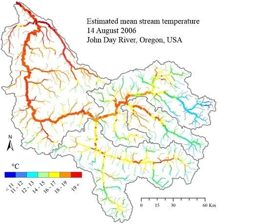
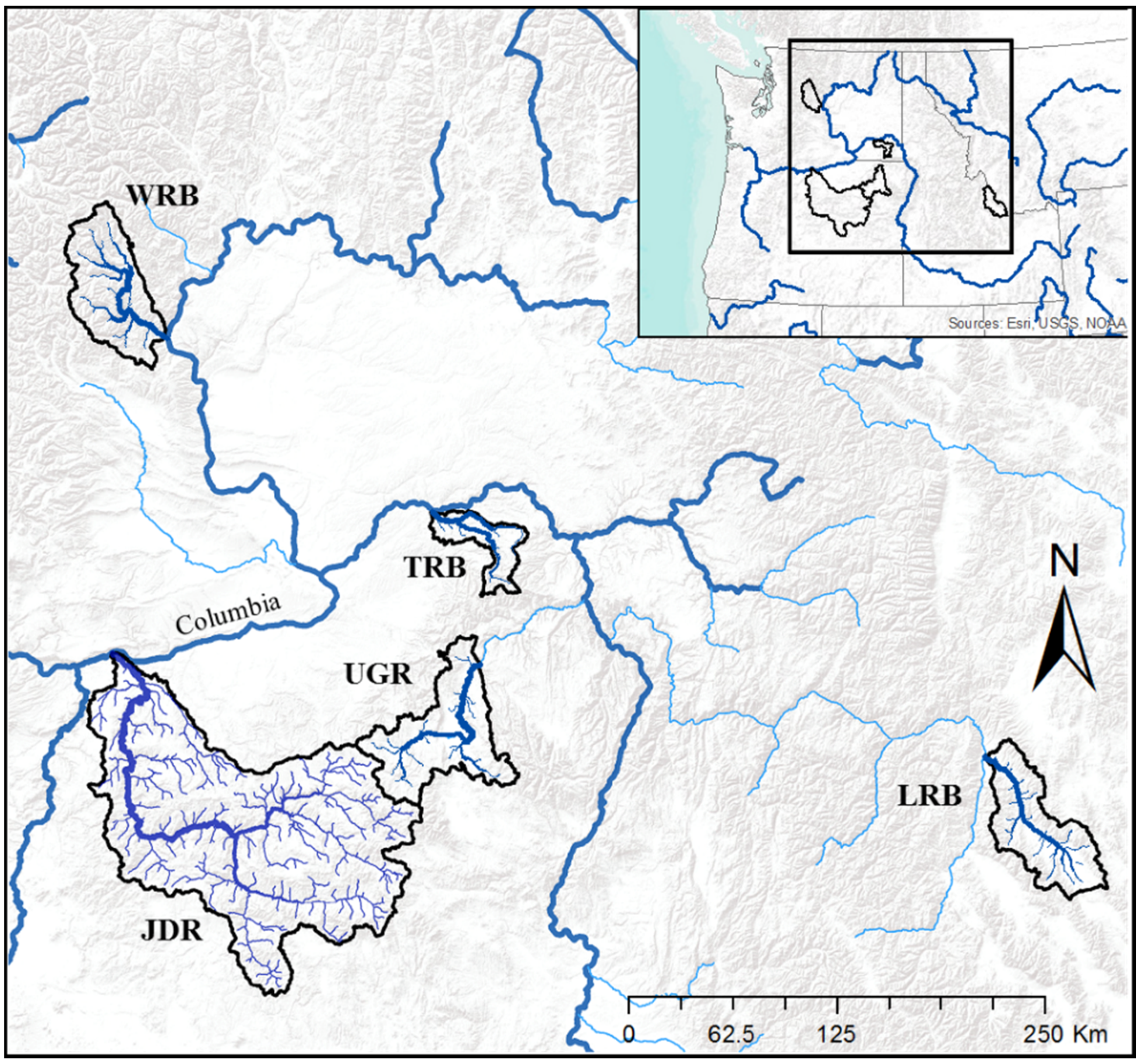
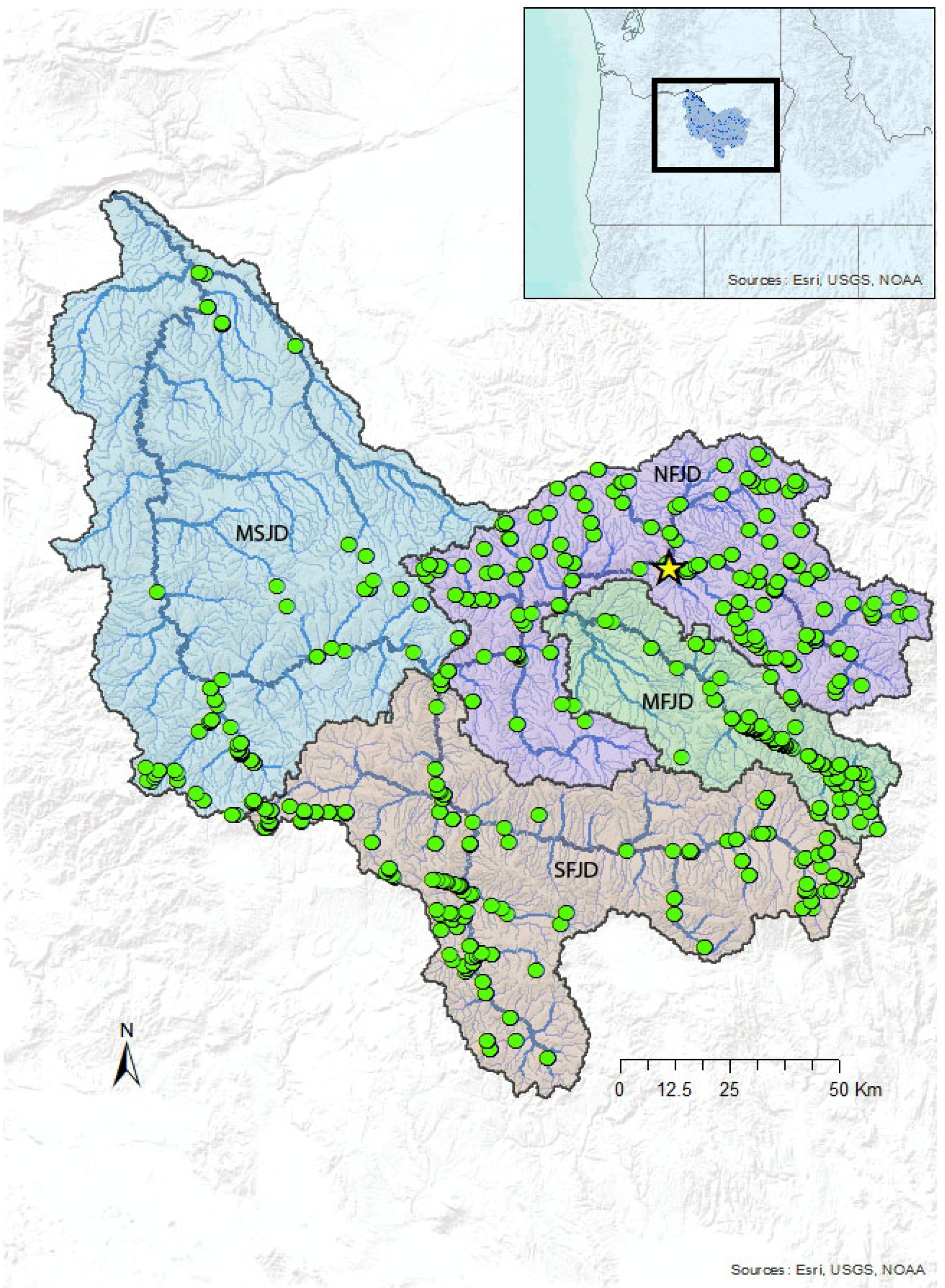
2. Study Area

3. Materials and Methods
3.1. Geospatial Data
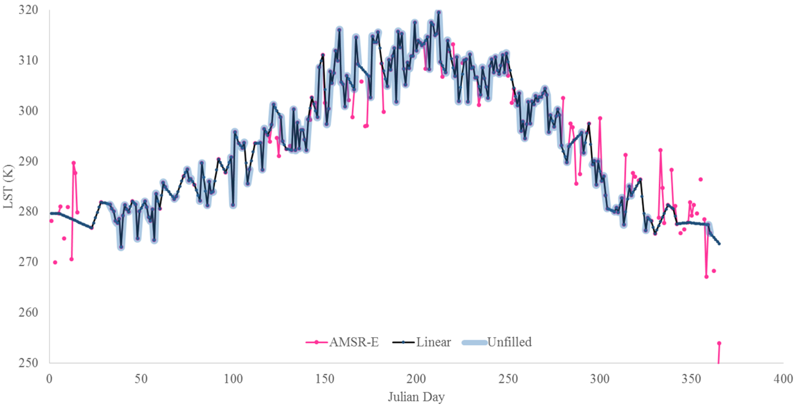
3.2. Land Surface Temperature Data and Handling Data Gaps

3.3. In-Stream Thermal Logger Data

| Year | 2000 | 2001 | 2002 | 2003 | 2004 | 2005 | 2006 | 2007 | 2008 | 2009 | Total |
|---|---|---|---|---|---|---|---|---|---|---|---|
| Sites | 50 | 64 | 72 | 46 | 54 | 24 | 31 | 45 | 45 | 89 | 520 |
| Days | 6200 | 11,470 | 10,869 | 7667 | 5705 | 4658 | 4494 | 7195 | 9991 | 11,541 | 79,790 |
3.4. Model Development
- Temp ~ LST
- Temp ~ LST + LST2
- Temp ~ LST + JulianDay
- Temp ~ LST + JulianDay + Elevation
- Temp ~ LST + LST2 + JulianDay + Elevation
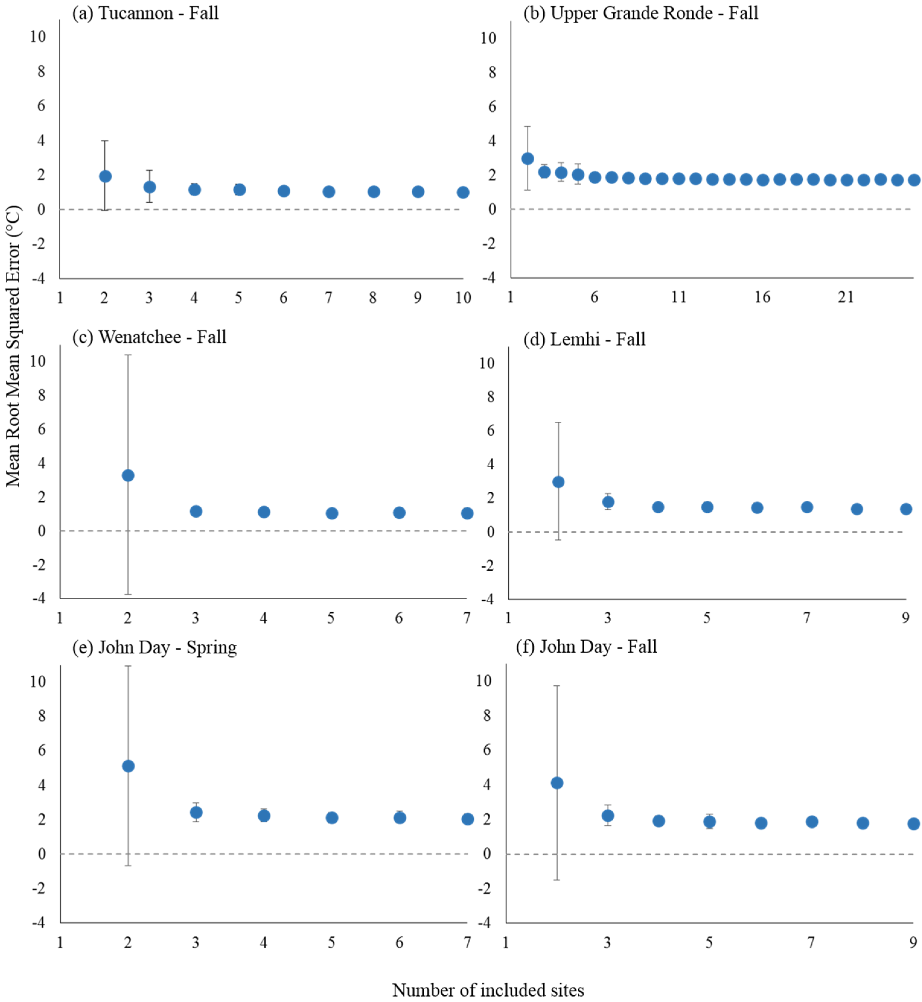
3.5. Sensitivity Analysis
4. Results
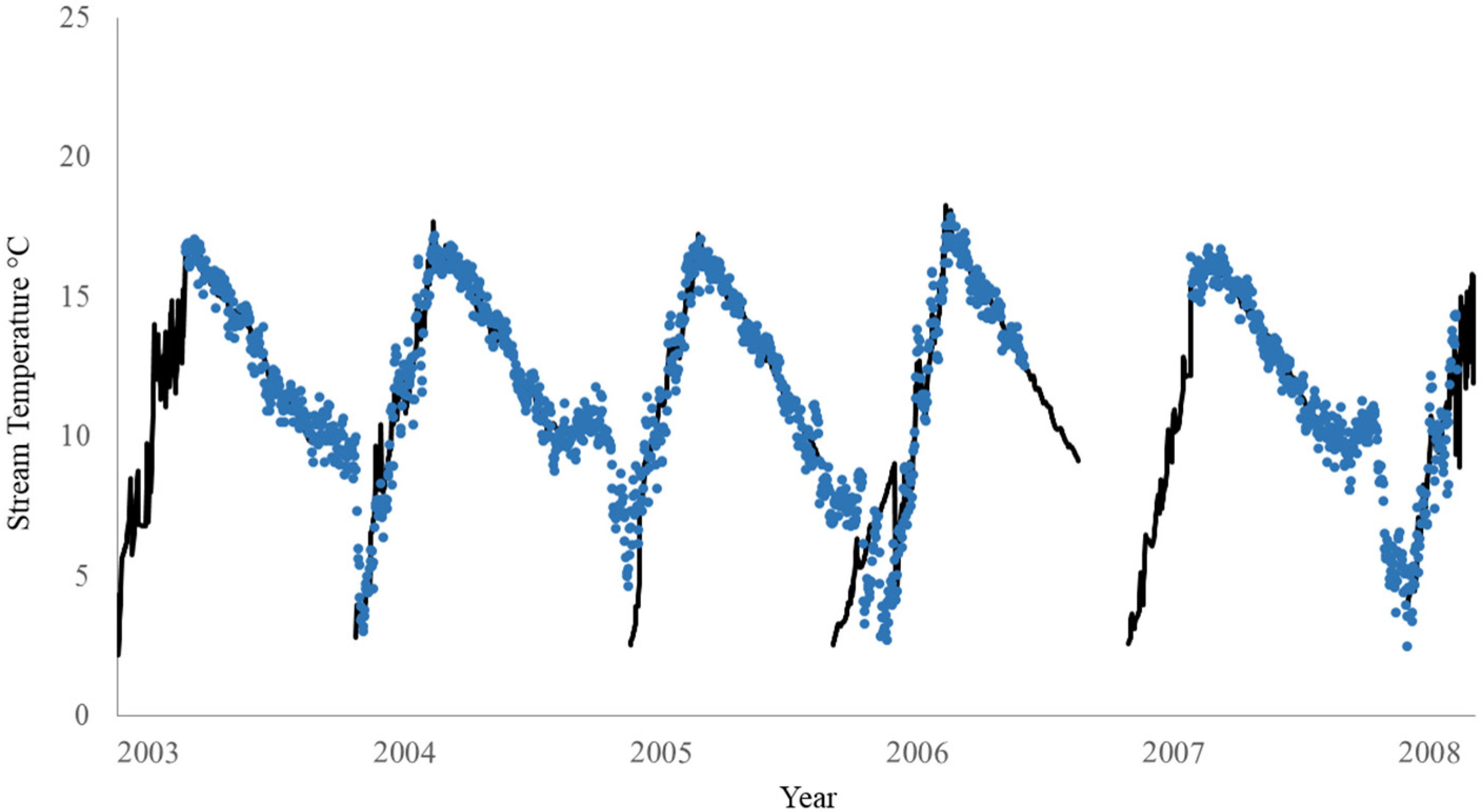
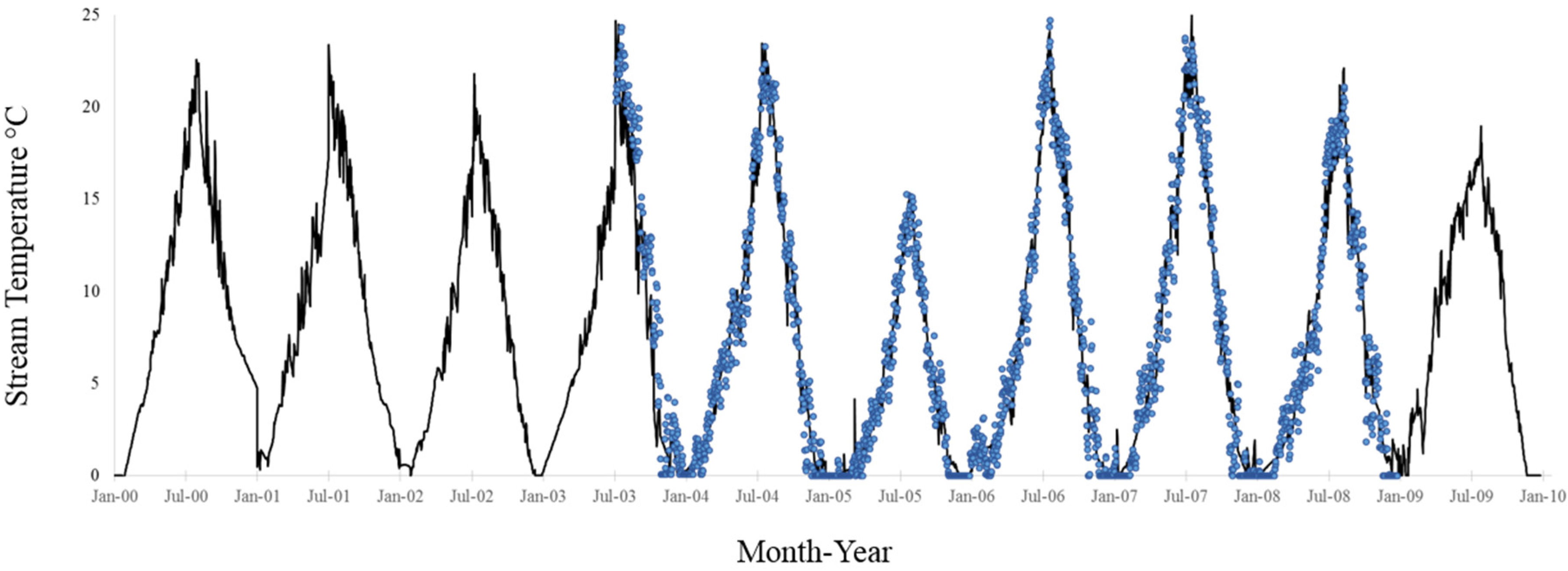
4.1. Estimating Missing Land Surface Temperature Data
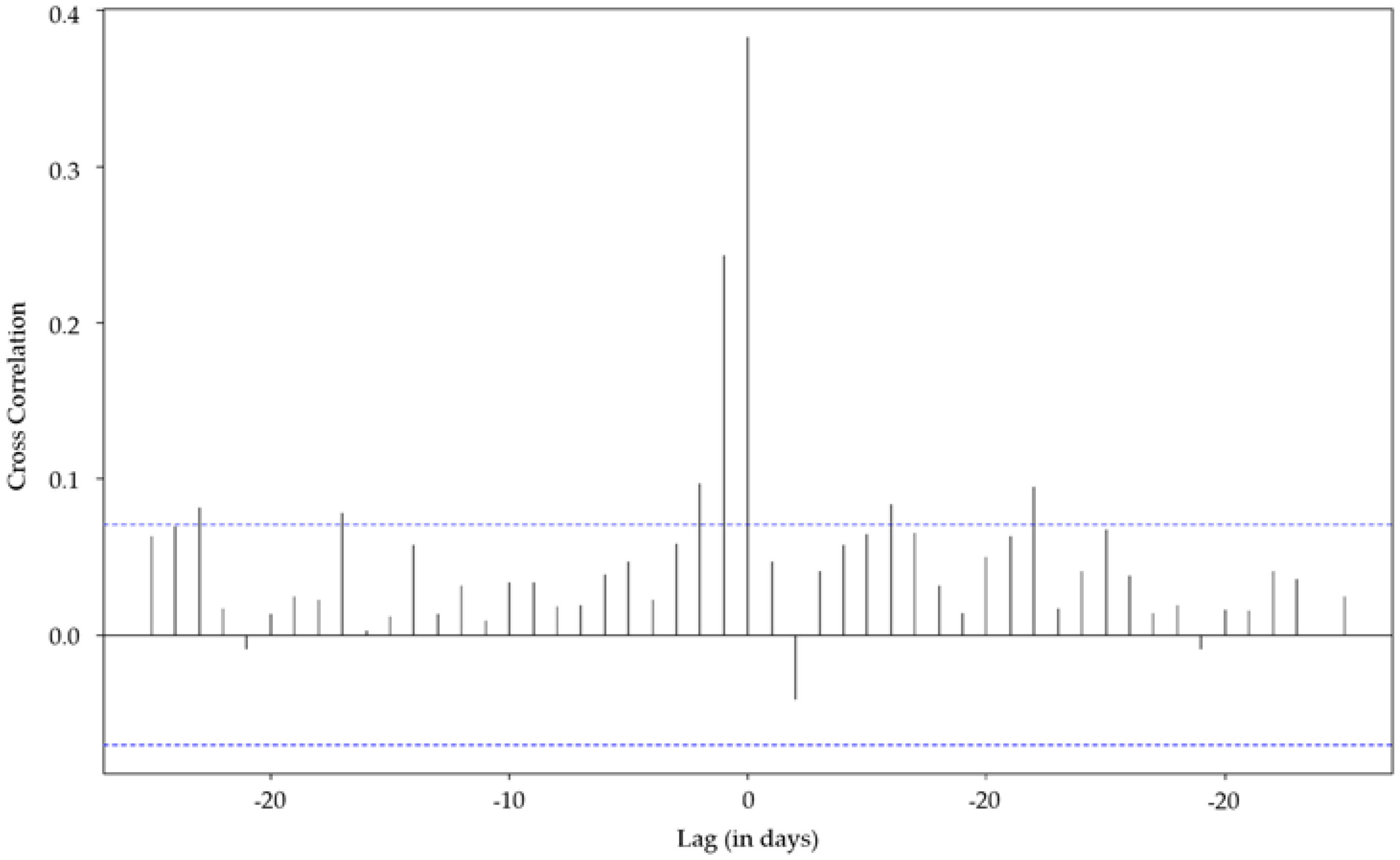
4.2. Predictor Variable Selection and Temporal Lag Analyses

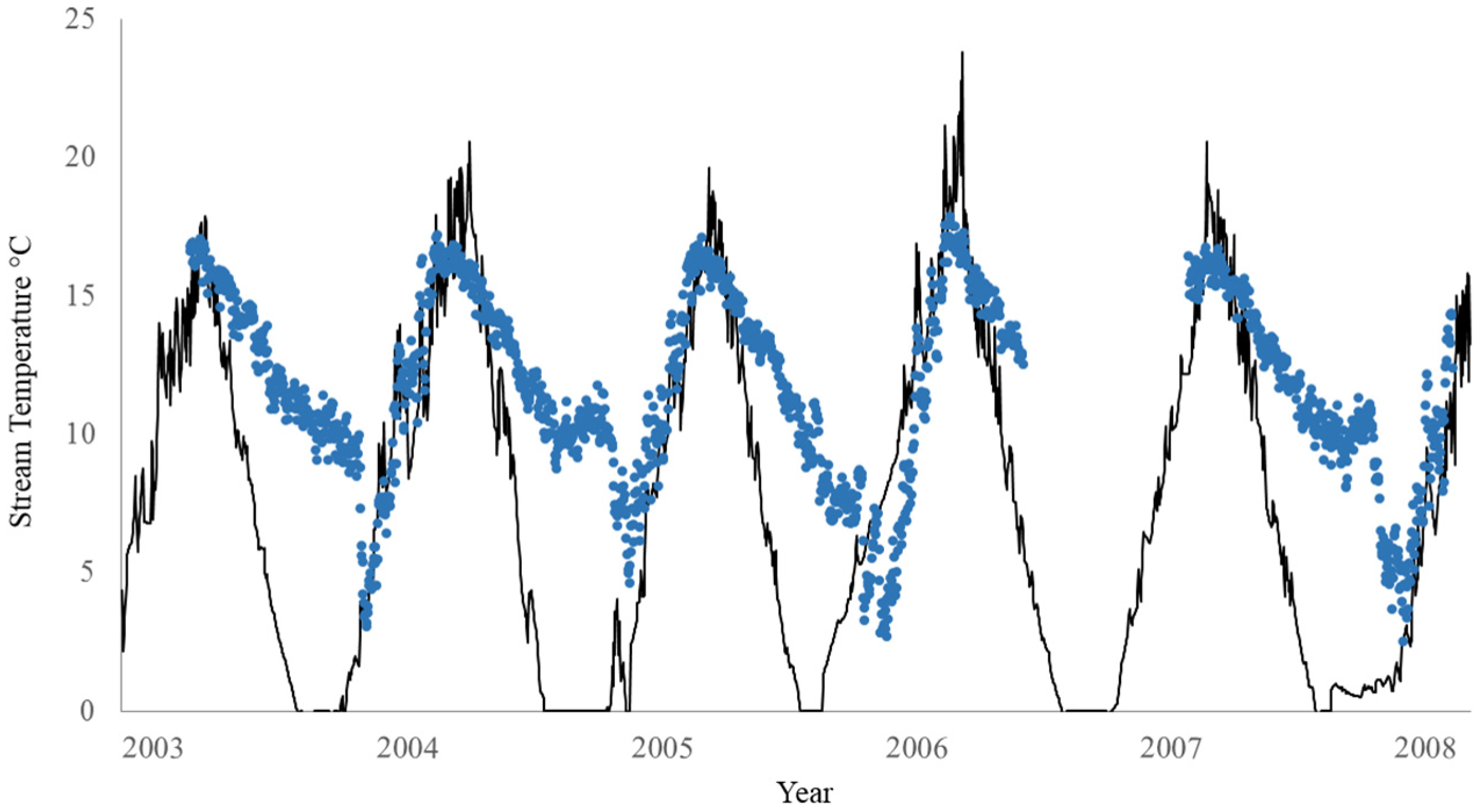
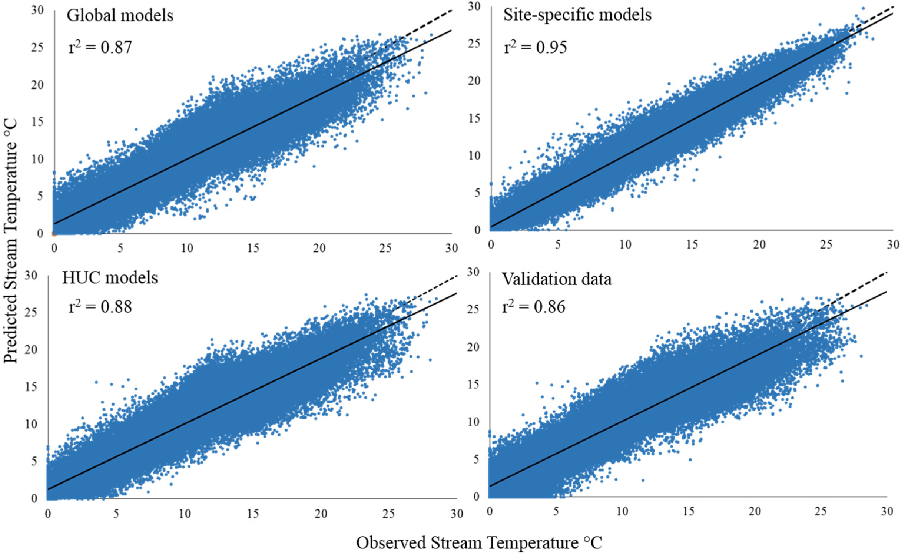
4.3. Daily Model Performance Across Temporal Scales in the JDR
| Model | Fixed Effects | N = 79,790 Days | |
|---|---|---|---|
| r2 | RMSE | ||
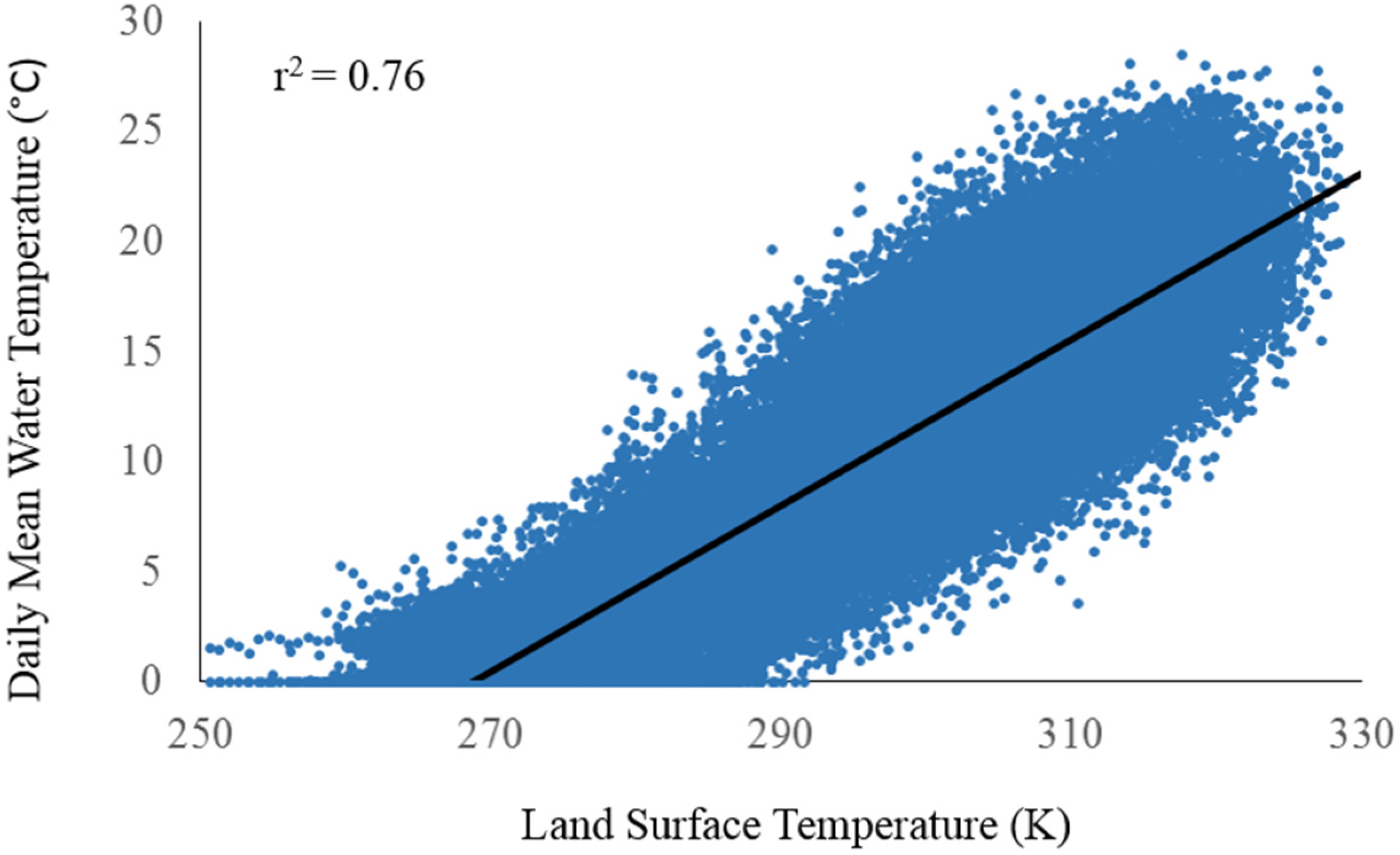
| OLS | DMWT ~ LST | 0.76 | 2.74 |
| OLS | DMWT ~ LST + year | 0.77 | 2.85 |
| OLS | DMWT ~ LST + year + season | 0.77 | 2.85 |
| Tobit | DMWT ~ LST | 0.76 | 2.80 |
| Tobit | DMWT ~ LST + year | 0.77 | 2.75 |
| Tobit | DMWT ~ LST + year + season | 0.76 | 2.80 |
| Model | Fixed Effects | RMSE | r2 |
|---|---|---|---|
| Global | DMWT ~ LST | 2.74 | 0.76 |
| Global | DMWT ~ LST + year | 2.85 | 0.77 |
| Global | DMWT ~ LST + year + season | 2.85 | 0.77 |
| Global | DMWT ~ LST + LST2 + Elev | 2.83 | 0.77 |
| Spring | DMWT ~ LST + LST2 + Elev + JulDay | 2.63 | 0.82 |
| Fall | DMWT ~ LST + LST2 + Elev + JulDay | 2.33 | 0.82 |
| Year | DMWT ~ LST + LST2 + Elev + JulDay | 2.24 | 0.83 |
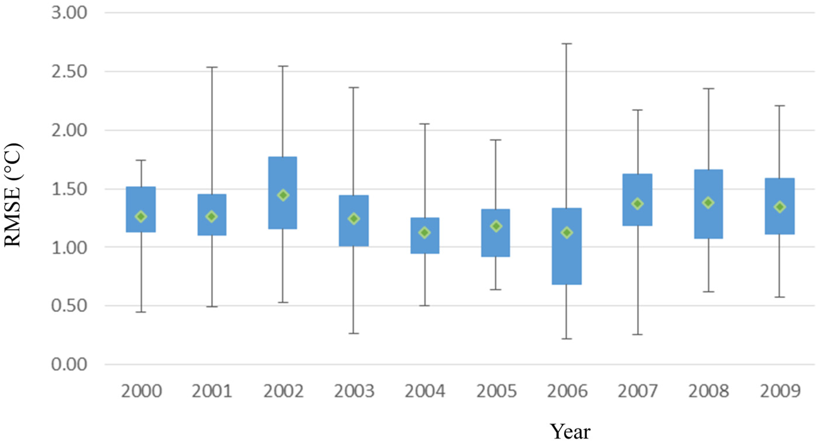
4.4. Annual, Daily Model Performance across Spatial Scales in the John Day River Basin

| Year | AMDM | AUC January–April | AUC January–June | AUC July–December | AUC Total |
|---|---|---|---|---|---|
| 2000 | 22.3 | 290 | 1209 | 2281 | 3491 |
| 2001 | 22.9 | 392 | 1332 | 1899 | 3232 |
| 2002 | 21.1 | 244 | 1068 | 1621 | 2688 |
| 2003 | 24.3 | 376 | 1270 | 1649 | 2919 |
| 2004 | 23.1 | 267 | 839 | 2128 | 2967 |
| 2005 | 15.3 | 63 | 431 | 1148 | 1579 |
| 2006 | 24.0 | 218 | 1037 | 1812 | 2849 |
| 2007 | 24.4 | 225 | 1175 | 1849 | 3024 |
| 2008 | 22.0 | 132 | 660 | 1887 | 2547 |
| 2009 | 18.3 | 395 | 998 | 1919 | 2917 |
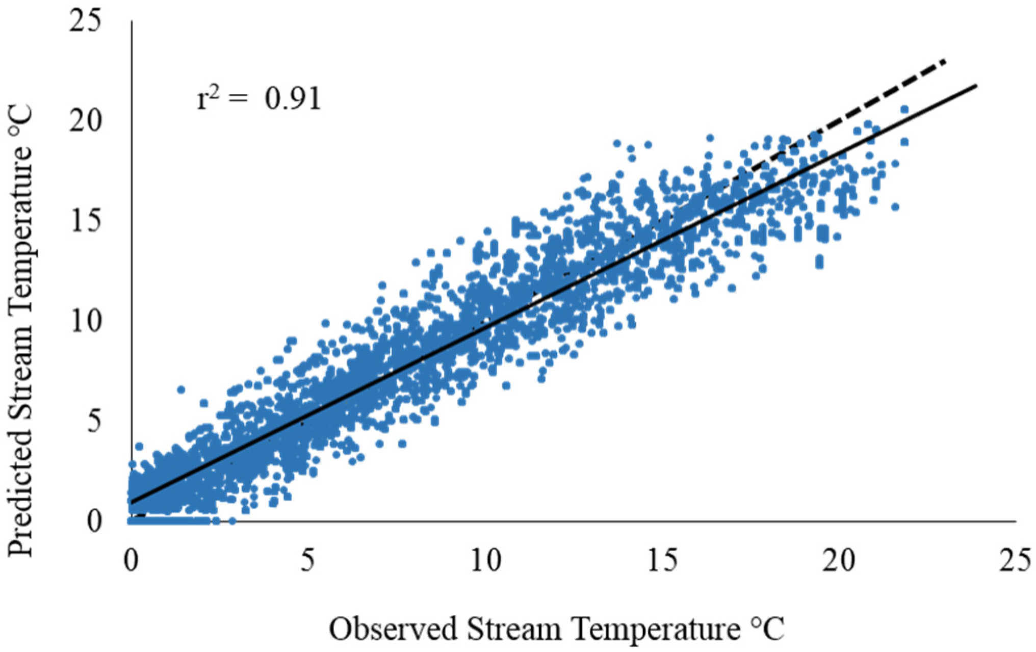
4.5. Eight-Day Model Performance and Sensitivity Analysis across Basins

| Basin | “Spring” | “Fall” | ||||||||
|---|---|---|---|---|---|---|---|---|---|---|
| N Sites | RMSE | r2 | RMSEP | p2 | N Sites | RMSE | r2 | RMSEP | p2 | |
| JDR | 11 | 1.70 | 0.91 | 2.38 | 0.91 | 18 | 1.56 | 0.93 | 2.33 | 0.92 |
| LRB | 0 | - | - | - | - | 18 | 1.22 | 0.91 | 2.32 | 0.91 |
| TRB | 10 | 1.32 | 0.91 | 1.96 | 0.90 | 20 | 0.97 | 0.96 | 1.97 | 0.96 |
| UGR | 31 | 1.80 | 0.88 | 2.66 | 0.88 | 52 | 1.65 | 0.92 | 2.74 | 0.92 |
| WRB | 9 | 0.81 | 0.95 | 1.20 | 0.95 | 8 | 0.90 | 0.94 | 1.75 | 0.94 |
5. Discussion


Acknowledgments
Author Contributions
Conflicts of Interest
References
- Beacham, T.D.; Murray, C.B. Temperature, Egg Size, and Development of Embryos and Alevins of Five Species of Pacific Salmon: A Comparative Analysis. Trans. Am. Fish. Soc. 1990, 119, 927–945. [Google Scholar] [CrossRef]
- Crossin, G.T.; Hinch, S.G.; Cooke, S.J.; Welch, D.W.; Patterson, D.A.; Jones, S.R.M.; Lotto, A.G.; Leggatt, R.A.; Mathes, M.T.; Shrimpton, J.M.; et al. Exposure to high temperature influences the behaviour, physiology and survival of sockeye salmon during spawning migration. Can. J. Zool. 2008, 86, 127–140. [Google Scholar] [CrossRef]
- Gadomski, D.M.; Caddell, S.M. Effects of temperature on early-life history stages of California halibut Paralichthys californicus. Fish. Bull. 1991, 89, 567–576. [Google Scholar]
- Beauchamp, D.A.; Cross, A.D.; Armstrong, J.L.; Myers, K.W.; Moss, J.H.; Boldt, J.L.; Haldorson, L.J. Bioenergetic responses by Pacific salmon to climate and ecosystem variation. N. Pac. Anadromous Fish Comm. Bull. 2007, 4, 257–269. [Google Scholar]
- Arismendi, I.S.L.J.; Dunham, J.B.; Haggerty, R. Descriptors of natural thermal regimes in streams and responsiveness to change in the Pacific Northwest of America. Freshw. Biol. 2013, 58, 880–894. [Google Scholar] [CrossRef]
- State of Oregon Department of Environmental Quality. Methodology for Oregon’s Water Quality Report and List of Water Quality Limited Waters; State of Oregon Department of Environmental Quality: Portland, OR, USA, 2014.
- Poole, G.C.; Dunham, J.B.; Keenan, D.M.; Sauter, S.T.; McCullough, D.A.; Mebane, C.; Lockwood, J.C.; Essig, D.A.; Hicks, M.P.; Sturdevant, D.J.; et al. The Case for Regime-based Water Quality Standards. BioScience 2004, 54, 155–161. [Google Scholar] [CrossRef]
- Caissie, D. The thermal regime of rivers: A review. Freshw. Biol. 2006, 51, 1389–1406. [Google Scholar] [CrossRef]
- Faush, K.D.; Torgersen, C.E.; Baxter, C.V.; Li, H.W. Landscapes to riverscapes: Bridging the gap between research and conservation of stream fishes. BioScience 2002, 52, 483–498. [Google Scholar] [CrossRef]
- Crozier, L.G.; Zabel, R.W. Climate impacts at multiple scales: Evidence for differential population responses in juvenile Chinook salmon. J. Anim. Ecol. 2006, 75, 1100–1109. [Google Scholar] [CrossRef] [PubMed]
- Crozier, L.G.; Hendry, A.P.; Lawson, P.W.; Quinn, T.P.; Mantua, N.J.; Battin, J.; Shaw, R.G.; Huey, R.B. Potential responses to climate change in organisms with complex life histories: Evolution and plasticity in Pacific salmon. Evol. Appl. 2008, 1, 252–270. [Google Scholar] [CrossRef] [PubMed]
- Olden, J.D.; Naiman, R.J. Incorporating thermal regimes into environmental flows assessments: Modifying dam operations to restore freshwater ecosystem integrity. Freshw. Biol. 2010, 55, 86–107. [Google Scholar] [CrossRef]
- Dunham, J.; Chandler, G.; Rieman, B.; Martin, D. Measuring Stream Temperature with Digital Data Loggers: A User’s Guide; U.S. Department of Agriculture, Forest Service, Rocky Mountain Research Station: Fort Collins, CO, USA, 2005.
- Torgersen, C.E.; Faux, R.N.; McIntosh, B.A.; Poage, N.J.; Dj, N. Airborne thermal remote sensing for water temperature assessment in rivers and streams. Remote Sens. Environ. 2001, 76, 386–398. [Google Scholar] [CrossRef]
- Torgersen, C.E.; Ebersole, J.L.; Keenan, D. Primer for Identifying Cold-Water Refuges to Protect and Restore Thermal Diversity in Riverine Landscapes; EPA 910-C-12-001; U.S. Environmental Protection Agency: Washington, DC, USA, 2012.
- Vatland, S.J.; Gresswell, R.E.; Poole, G.C. Quantifying stream thermal regimes at multiple scales: Combining thermal infrared imagery and stationary stream temperature data in a novel modeling framework. Water Resour. Res. 2015, 51, 31–46. [Google Scholar] [CrossRef]
- Poole, G.C.; Berman, C.H. An ecological perspective on in-stream temperature: Natural heat dynamics and mechanisms of human-caused thermal degradation. Environ. Manag. 2001, 27, 787–802. [Google Scholar] [CrossRef]
- Arismendi, I.M.S.; Dunham, J.B.; Johnson, S.L. Can air temperature be used to project influences of climate change on stream temperature? Environ. Res. Lett. 2014, 9, 1–12. [Google Scholar] [CrossRef]
- Snyder, C.D.; Hitt, N.P.; Young, J.A. Accounting for groundwater in stream fish thermal habitat responses to climate change. Ecol. Appl. 2015, 25, 1397–1419. [Google Scholar] [CrossRef] [PubMed]
- Fullerton, A.H.; Torgersen, C.E.; Lawler, J.J.; Faux, R.N.; Steel, E.A.; Beechie, T.J.; Ebersole, J.L.; Leibowitz, S.G. Rethinking the longitudinal stream temperature paradigm: Region-wide comparison of thermal infrared imagery reveals unexpected complexity of river temperatures. Hydrol. Process. 2015, 29, 4719–4737. [Google Scholar] [CrossRef]
- Pike, A.; Danner, E.; Boughton, D.; Melton, F.; Nemani, R.; Rajagopalan, B.; Lindley, S. Forecasting river temperatures in real time using a stochastic dynamics approach. Water Resour. Res. 2013, 49, 5168–5182. [Google Scholar] [CrossRef]
- Yearsley, J.R. A semi-Lagrangian water temperature model for advection-dominated river systems. Water Resour. Res. 2009, 45. [Google Scholar] [CrossRef]
- Gardner, B.; Sullivan, P.J.; Lembo, J. Predicting stream temperatures: Geostatistical model comparison using alternative distance metrics. Can. J. Fish. Aquat. Sci. 2003, 60, 344–351. [Google Scholar] [CrossRef]
- Isaak, D.J.; Luce, C.H.; Rieman, B.E.; Nagel, D.E.; Peterson, E.E.; Horan, D.L.; Parkes, S.; Chandler, G.L. Effects of climate change and wildfire on stream temperatures and salmonid thermal habitat in a mountain river network. Ecol. Appl. 2010, 20, 1350–1371. [Google Scholar] [CrossRef] [PubMed]
- Isaak, D.J.; Peterson, E.; Hoef, J.V.; Wenger, S.; Falke, J.; Torgersen, C.; Sowder, C.; Steel, A.; Fortin, M.J.; Jordan, C.; et al. Applications of spatial statistical network models to stream data. WIREs Water 2014, 1, 277–294. [Google Scholar] [CrossRef]
- Peterson, E.E.; ver Hoef, J.M.; Isaak, D.J.; Falke, J.A.; Fortin, M.-J.; Jordan, C.E.; McNyset, K.; Monestiez, P.; Ruesch, A.S.; Sengupta, A.; et al. Modelling dendritic ecological networks in space: An integrated network perspective. Ecol. Lett. 2013, 16, 707–719. [Google Scholar] [CrossRef] [PubMed]
- Kay, J.E.; Kampf, S.K.; Handcock, R.N.; Cherkauer, K.A.; Gillespie, A.R.; Burges, S.J. Accuracy of lake and stream temperatures estimated from thermal infrared images. J. Am. Water Resour. Assoc. 2005, 41, 1161–1175. [Google Scholar] [CrossRef]
- Wan, Z. Collection-5 MODIS Land Surface Temperature Products Users’ Guide; ICESS University of California: Santa Barbara, CA, USA, 2007. [Google Scholar]
- Wan, Z.; Dozier, J. A generalized split-window algorithm for retrieving land-surface temperature from space. IEEE Trans. Geosci. Remote Sens. 1996, 34, 892–905. [Google Scholar]
- Minnett, P.J.; Brown, O.B.; Evans, R.H.; Key, E.L.; Kearns, E.J.; Kilpatrick, K.; Kumar, A.; Maillet, K.A.; Szczodrak, G. Sea-surface temperature measurements from the Moderate-Resolution Imaging Spectroradiometer (MODIS) on Aqua and Terra. In Proceedings of the IEEE International Geoscience and Remote Sensing Symposium, Anchorage, AK, USA, 20–24 September 2004; Volume 7, pp. 4576–4579.
- Benke, A.C. A perspective on America’s vanishing streams. J. N. Am. Benthol. Soc. 1990, 9, 77–88. [Google Scholar] [CrossRef]
- United States, Department of Interior. Record of Decision: John Day River Management Plan, Two Rivers Resource Management Plan Amendment, John Day Resource Management Plan Amendment, & Baker Resource Management Plan Amendment; Bureau of Land Management: Prineville, OR, USA, 2001.
- Upper John Day River Local Advisory Committee. Upper Mainstem and South Fork John Day River Agricultural Water Quality Management Area Plan; Oregon Department of Agriculture: Salem, OR, USA, 2015.
- Covert, J.; Lyerla, J.; Ader, M. Initial Watershed Assessment: Tucannon River Watershed; Washington Department of Ecology, Eastern Regional Office, Water Resources Program: Spokane, WA, USA, 1995.
- Bohle, T.S. Stream Temperatures, Riparian Vegetation, and Channel Morphology in the Upper Grande Ronde River Watershed; Department of Forest Engineering, Oregon State University: Corvallis, OR, USA, 1994. [Google Scholar]
- Oregon Geospatial Enterprise Office Digital Elevation Models (DEM). Available online: http://www.oregon.gov/DAS/CIO/GEO/pages/data/dems.aspx (accessed on 2 December 2015).
- Environmental Systems Research Institute. ArcGIS; Environmental Systems Research Institute: Redlands, CA, USA, 2009. [Google Scholar]
- Theobald, D.M.J.B.N.; Peterson, E.E.; Ferraz, S.; Wade, A.; Sherburne, M.R. Functional Linkage of Waterbasins and Streams (FloWs) v1 User’s Guide: ArcGIS Tools for Network-Based Analysis of Freshwater Ecosystems; Natural Resources Ecology Lab, Colorado State University: Fort Collins, CO, USA, 2006. [Google Scholar]
- Gesch, D.; Oimoen, M.; Greenlee, S.; Nelson, C.; Steuck, M.; Tyler, D. The national elevation dataset. Photogramm. Eng. Remote Sens. 2002, 68, 5–32. [Google Scholar]
- Earth Observing System Data and Information System (EOSDIS) Earth Observing System Data and Information System (EOSDIS). Available online: http://reverb.echo.nasa.gov/ (accessed on 2 December 2015).
- Environmental Systems Research Institute. ArcGIS 10.2.2 for Desktop; Environmental Systems Research Institute, Inc.: Redlands, CA, USA, 1999. [Google Scholar]
- Roberts, J.J.; Best, B.D.; Dunn, D.C.; Treml, E.A.; Halpin, P.N. Marine Geospatial Ecology Tools: An integrated framework for ecological geoprocessing with ArcGIS, Python, R, MATLAB, and C++. Environ. Model. Softw. 2010, 25, 1197–1207. [Google Scholar] [CrossRef]
- Wan, Z. New refinements and validation of the MODIS Land-Surface Temperature/Emissivity products. Remote Sens. Environ. 2008, 112, 59–74. [Google Scholar] [CrossRef]
- Coll, C.; Wan, Z.; Galve, J.M. Temperature-based and radiance-based validations of the V5 MODIS land surface temperature product. J. Geophys. Res. 2009, 114. [Google Scholar] [CrossRef]
- Mao, K.; Shi, J.; Li, Z.; Qin, Z.; Li, M.; Xu, B. A physics-based statistical algorithm for retrieving land surface temperature from AMSR-E passive microwave data. Sci. China Ser. Earth Sci. 2007, 50, 1115–1120. [Google Scholar] [CrossRef]
- Mcfarland, M.J.; Miller, R.L.; Neale, C.M.U. Land surface temperature derived from the SSM/I passive microwave brightness temperatures. IEEE Trans. Geosci. Remote Sens. 1990, 28, 839–845. [Google Scholar] [CrossRef]
- Knowles, K.; Savoie, M.; Armstrong, R.; Brodzik, M. AMSR-E/Aqua Daily EASE-Grid Brightness Temperatures, Version 1. January to December 2003. Available online: http://dx.doi.org/10.5067/XIMNXRTQVMOX (accessed on 1 February 2011).
- Wuertz, D.; Chalabi, Y. Rmetrics-Financial Time Series Objects, R package version 3010.97; The Comprehensive R Archive Network, Institute for Statistics and Mathematics: Wien, Austria, 2013. [Google Scholar]
- Dille, J.A.; Milner, M.; Groeteke, J.J.; Mortensen, D.A.; Williams, I.I.; Martin, M. How good is your weed map? A comparison of spatial interpolators. Weed Sci. 2003, 51, 44–55. [Google Scholar] [CrossRef]
- Hwang, Y.; Clark, M.; Rajagopalan, B.; Leavesley, G. Spatial interpolation schemes of daily precipitation for hydrologic modeling. Stoch. Environ. Res. Risk Assess. 2012, 26, 295–320. [Google Scholar] [CrossRef]
- Integrated Status & Effectiveness Monitoring Program. Available online: www.isemp.org (accessed on 2 December 2015).
- Sowder, C.; Steel, E.A. A note on the collection and cleaning of water temperature data. Water 2012, 4, 597–606. [Google Scholar] [CrossRef]
- Stevens, D.L.; Olsen, A.R. Variance estimation for spatially balanced samples of environmental resources. Environmetrics 2003, 14, 593–610. [Google Scholar] [CrossRef]
- Isaak, D.J.; Hubert, W.A. A hypothesis about factors that affect stream temperatures across montane landscapes. J. Am. Water Resour. Assoc. 2001, 37, 351–366. [Google Scholar] [CrossRef]
- Chan, K.-S.; Ripley, B. TSA: Timer Series Analysis, R package version 1.01; The Comprehensive R Archive Network, Institute for Statistics and Mathematics: Wien, Austria, 2012. [Google Scholar]
- Cryer, J.D.; Chan, K. Time Series Analysis with Applications in R, 2nd ed.; Springer: Berlin, Germany, 2008. [Google Scholar]
- Tobin, J. Estimation of Relationships for Limited Dependent Variables. Econometrica 1958, 26, 24–36. [Google Scholar] [CrossRef]
- Amemiya, T. Tobit models: A survey. J. Econom. 1984, 24, 3–61. [Google Scholar] [CrossRef]
- Yee, T.W. VGAM: Vector Generalized Linear and Additive Models, R package version 0.9-5; The Comprehensive R Archive Network, Institute for Statistics and Mathematics: Wien, Austria, 2014. [Google Scholar]
- Seaber, P.R.; Kapinos, F.P.; Knapp, G.L. Hydrologic Unit Maps; U.S. Geological Survey: Reston, VA, USA, 1987.
- Akaike, H. A new look at the statistical model identification. IEEE Trans. Autom. Control 1974, 19, 716–723. [Google Scholar] [CrossRef]
- Maheu, A.; Poff, N.L.; St-Hilaire, A. A Classification of Stream Water Temperature Regimes in the Conterminous USA. River Res. Appl. Available online: http://onlinelibrary.wiley.com/doi/10.1002/rra.2906/abstract (accessed on 7 October 2015).
- Ward, J.V.; Stanford, J.A. Thermal Responses in the Evolutionary Ecology of Aquatic Insects. Annu. Rev. Entomol. 1982, 27, 97–117. [Google Scholar] [CrossRef]
- Miller, P.; Lanier, W.; Brandt, S. Using Growing Degree Days to Predict Plant Stages; Montana State University-Bozeman: Bozeman, MO, USA, 2001. [Google Scholar]
© 2015 by the authors; licensee MDPI, Basel, Switzerland. This article is an open access article distributed under the terms and conditions of the Creative Commons by Attribution (CC-BY) license (http://creativecommons.org/licenses/by/4.0/).
Share and Cite
McNyset, K.M.; Volk, C.J.; Jordan, C.E. Developing an Effective Model for Predicting Spatially and Temporally Continuous Stream Temperatures from Remotely Sensed Land Surface Temperatures. Water 2015, 7, 6827-6846. https://doi.org/10.3390/w7126660
McNyset KM, Volk CJ, Jordan CE. Developing an Effective Model for Predicting Spatially and Temporally Continuous Stream Temperatures from Remotely Sensed Land Surface Temperatures. Water. 2015; 7(12):6827-6846. https://doi.org/10.3390/w7126660
Chicago/Turabian StyleMcNyset, Kristina M., Carol J. Volk, and Chris E. Jordan. 2015. "Developing an Effective Model for Predicting Spatially and Temporally Continuous Stream Temperatures from Remotely Sensed Land Surface Temperatures" Water 7, no. 12: 6827-6846. https://doi.org/10.3390/w7126660