
Distribution of Epilithic Diatoms in Estuaries of the Korean Peninsula in Relation to Environmental Variables


Abstract
:1. Introduction
2. Materials and Methods
2.1. Ecological Data

2.2. Data Analysis
3. Results
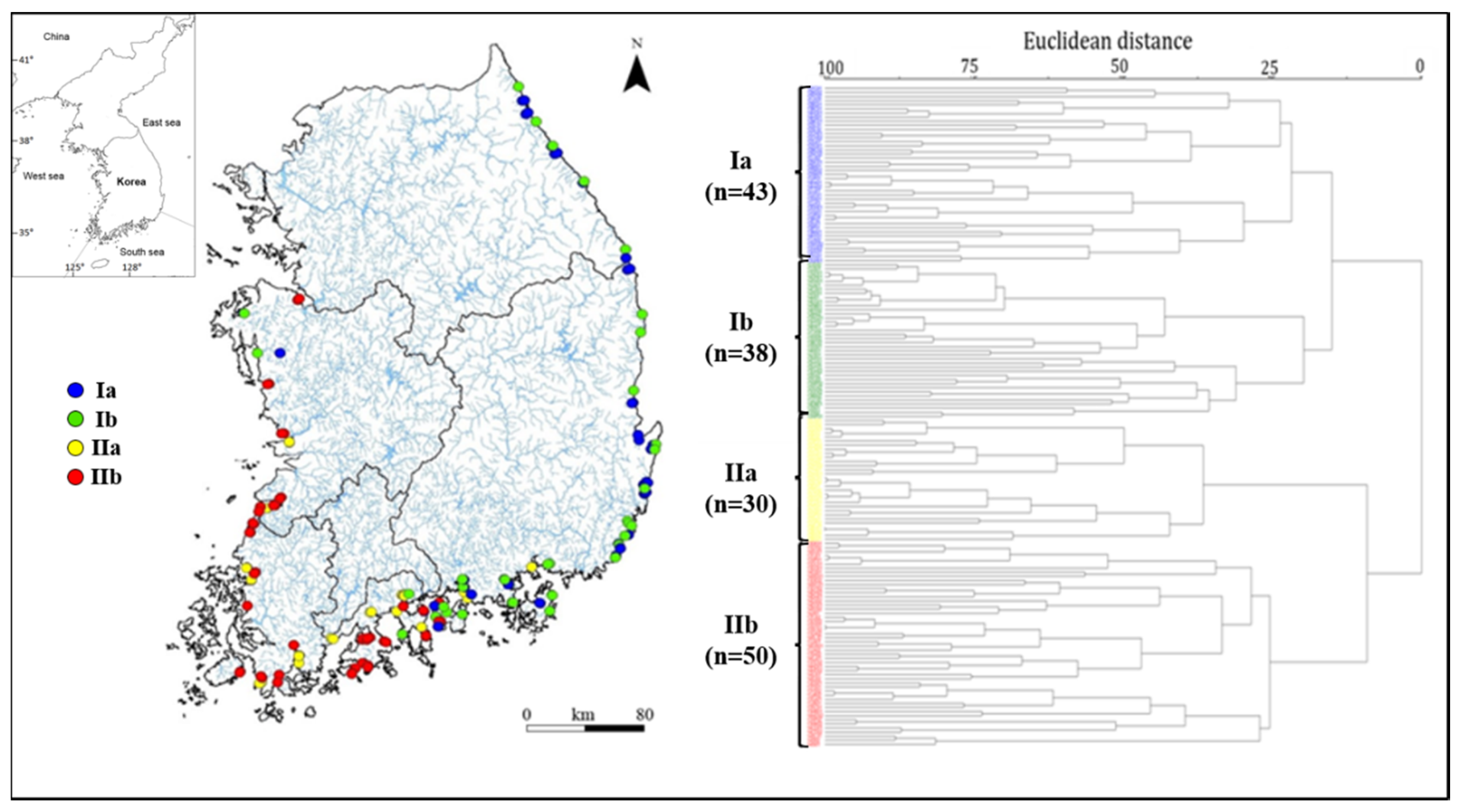
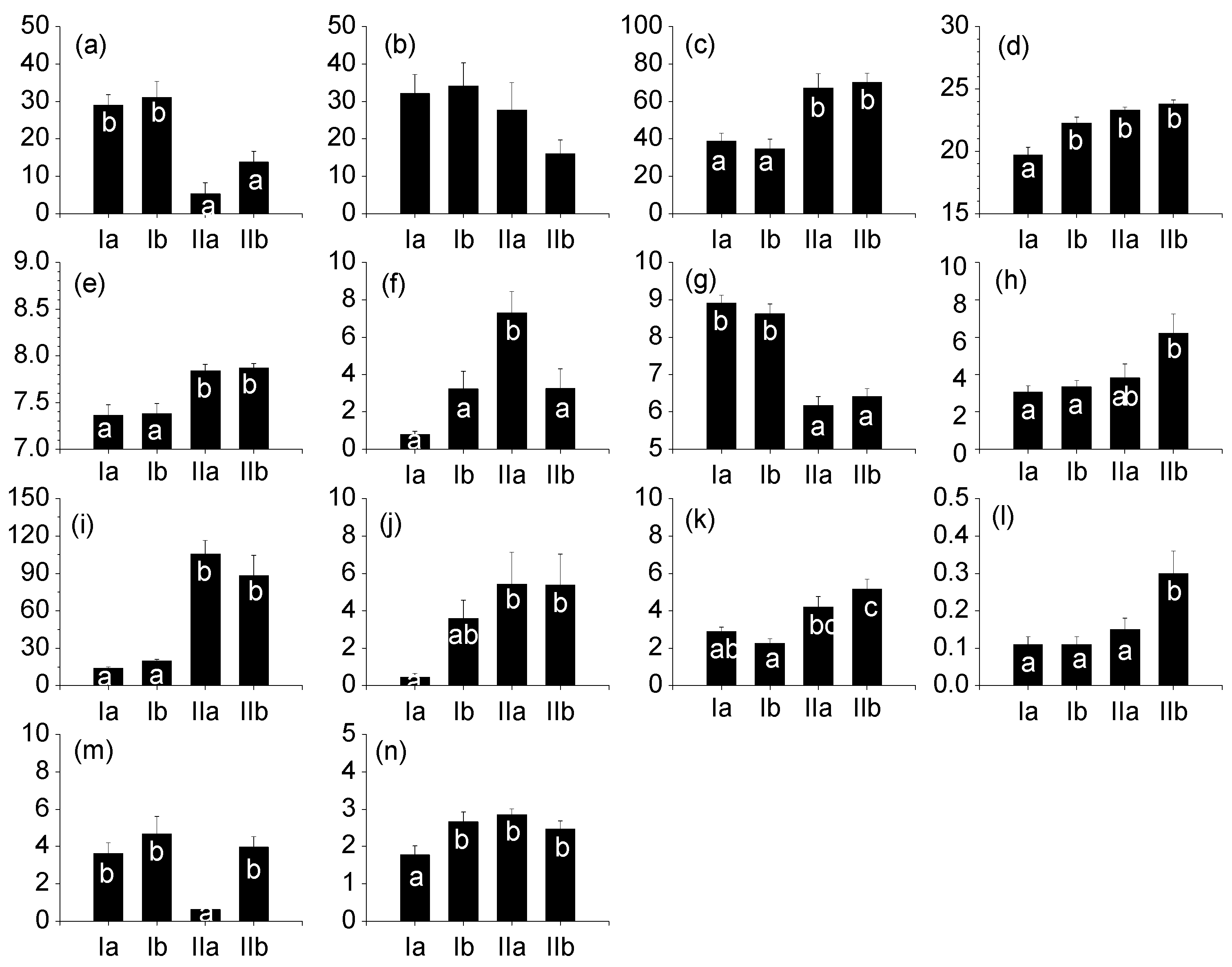
3.1. Characteristics of Epilithic Diatom Communities

| Variables | Groups | F ratio | P value | |||
|---|---|---|---|---|---|---|
| Ia | Ib | IIa | IIb | |||
| Biomass (103 cells /cm2) | 566.4 ± 70.3 | 500.5 ± 67.2 | 705.6 ± 178.1 | 505.4 ± 69.7 | 0.878 | 0.454 |
| Number of species (No. /cm2) | 31.23 ± 1.36 b | 30.76 ± 2.20 b | 24.27 ± 1.40 a | 20.56 ± 0.87 a | 13.572 | <0.001 |
| Dominance index (DI) | 0.58 ± 0.21 ab | 0.57 ± 0.03 ab | 0.63 ± 0.03 b | 0.50 ± 0.02 a | 4.543 | 0.004 |
| Diversity index (H’) | 2.06 ± 0.08 | 2.07 ± 0.10 | 1.84 ± 0.09 | 2.11 ± 0.07 | 1.708 | 0.168 |
| Richness (R) | 2.18 ± 0.09 b | 2.11 ± 0.16 b | 1.45 ± 0.11 a | 1.37 ± 0.06 a | 16.966 | <0.001 |
| Evenness (E) | 0.61 ± 0.02 a | 0.63 ± 0.02 a | 0.64 ± 0.03 a | 0.73 ± 0.02 b | 7.460 | <0.001 |
| Family | Groups | |||||||
|---|---|---|---|---|---|---|---|---|
| Ia | Ib | IIa | IIb | |||||
| N | D | N | D | N | D | N | D | |
| Achnanthaceae | 12.26 | 21.22 | 11.70 | 2.97 | 12.50 | 3.34 | 10.49 | 10.69 |
| Bacillariaceae | 13.55 | 37.78 | 19.15 | 57.78 | 13.28 | 61.74 | 14.20 | 42.76 |
| Entomoneidaceae | 0.00 | 0.00 | 1.06 | 0.22 | 1.56 | 0.01 | 0.00 | 0.00 |
| Eunotiaceae | 1.29 | 0.04 | 1.06 | 0.01 | 0.78 | 0.00 | 1.23 | 0.14 |
| Fragilariaceae | 18.06 | 12.28 | 11.17 | 9.37 | 10.16 | 3.49 | 14.81 | 2.69 |
| Hemidiscaceae | 0.65 | 0.03 | 0.00 | 0.00 | 0.00 | 0.00 | 0.00 | 0.00 |
| Melosiraceae | 1.29 | 1.21 | 2.13 | 2.46 | 1.56 | 0.62 | 1.23 | 2.73 |
| Naviculaceae | 46.45 | 27.15 | 47.34 | 25.02 | 43.75 | 26.29 | 47.53 | 34.44 |
| Surirellaceae | 1.94 | 0.07 | 1.60 | 0.10 | 4.69 | 0.06 | 1.85 | 0.37 |
| Thalassiosiraceae | 4.52 | 0.22 | 4.79 | 2.08 | 11.72 | 4.45 | 8.64 | 6.18 |
| Real N&D | 155 | 2.4 × 10⁷ | 188 | 1.8 × 10⁷ | 128 | 2.1 × 10⁷ | 162 | 2.5 × 10⁷ |
3.2. Differences in Environmental Factors
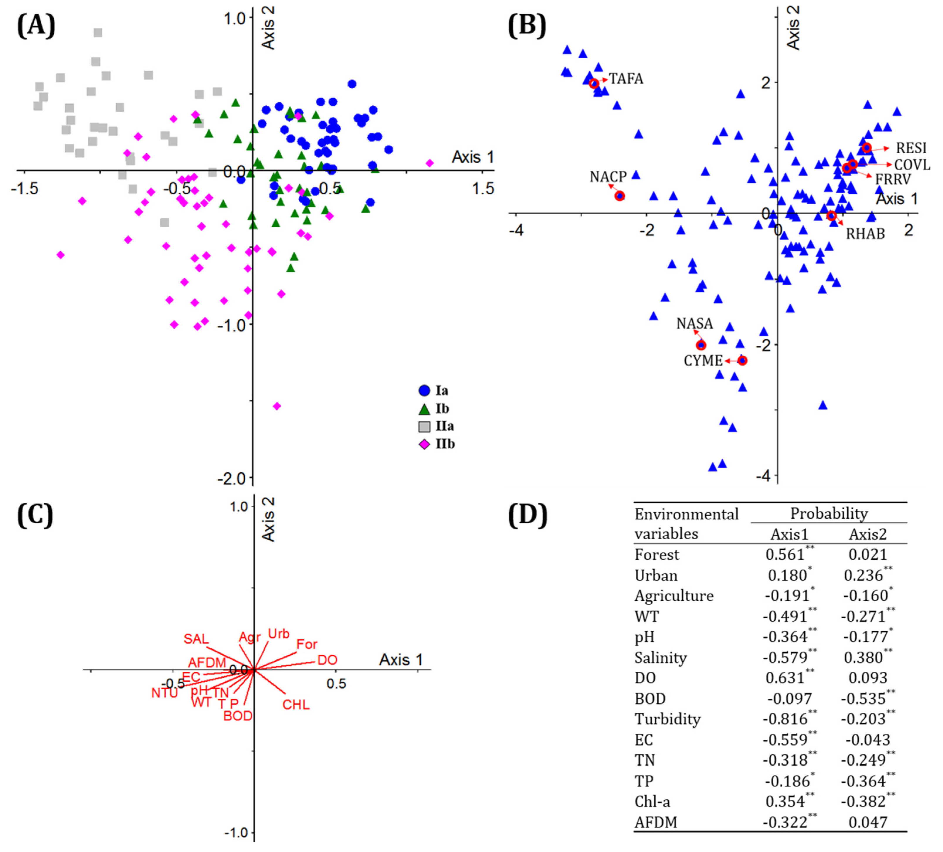
3.3. Correlations between Diatom Communities and Environment
| CODE | Forest | Urban | AGR | WT | pH | SAL | DO | BOD | TURB | EC | TN | TP | N/P | Chl-a | AFDM | Group |
|---|---|---|---|---|---|---|---|---|---|---|---|---|---|---|---|---|
| NASP | 0.27 ** | 0.18 * | −0.12 | −0.53 ** | −0.35 ** | −0.17 * | 0.44 ** | −0.11 | −0.45 ** | −0.35 ** | −0.11 | −0.15 | 0.15 | 0.06 | −0.34 ** | Ia |
| RESI | 0.33 ** | 0.07 | −0.06 | −0.34 ** | −0.19 * | −0.24 ** | 0.29 ** | −0.31 ** | −0.46 ** | −0.42 ** | −0.18 * | −0.25 ** | 0.20 * | 0.04 | −0.28 * | Ia |
| GOPS | 0.20 * | 0.21 ** | −0.16 * | −0.40 ** | −0.22 ** | −0.21 ** | 0.40 ** | −0.08 | −0.35 ** | −0.33 ** | −0.06 | −0.07 | 0.06 | 0.18 * | −0.22 ** | Ia |
| FRVG | 0.20 * | 0.18 * | −0.03 | −0.40 ** | −0.09 | −0.21 ** | 0.26 ** | −0.11 | −0.32 ** | −0.37 ** | −0.01 | −0.08 | 0.16 * | 0.12 | −0.28 ** | Ia |
| COVL | 0.18 * | 0.26 ** | −0.24 ** | −0.27 ** | −0.15 | −0.17 * | 0.19 * | −0.08 | −0.24 ** | −0.27 ** | 0.00 | −0.06 | 0.01 | 0.11 | −0.13 | Ia |
| NAMN | 0.14 | 0.17 * | −0.05 | −0.25 ** | −0.08 | −0.15 | 0.15 * | −0.16 * | −0.26 ** | −0.25 ** | 0.01 | −0.08 | 0.12 | 0.07 | −0.30 ** | Ia |
| NASU | 0.18 * | 0.19 * | −0.06 | −0.46 ** | −0.08 | −0.15 | 0.24 ** | −0.04 | −0.27 ** | −0.29 ** | 0.00 | −0.05 | 0.09 | 0.09 | −0.27 ** | Ia |
| FRRV | 0.13 | 0.24 ** | −0.21 ** | −0.40 ** | −0.13 | −0.13 | 0.27 ** | −0.14 | −0.27 ** | −0.27 ** | −0.09 | −0.13 | 0.11 | −0.01 | −0.32 ** | Ia |
| NASM | 0.14 | 0.18 * | −0.13 | −0.52 ** | 0.02 | −0.02 | 0.14 | −0.07 | −0.23 ** | −0.15 | 0.07 | −0.17 * | 0.26 ** | 0.02 | −0.35 ** | Ia |
| FRRU | 0.12 | 0.24 ** | −0.13 | −0.47 ** | −0.15 | −0.06 | 0.34 ** | −0.01 | −0.29 ** | −0.20 * | −0.08 | −0.18 * | 0.22 ** | −0.01 | −0.28 ** | Ia |
| ACSU | 0.14 | 0.03 | 0.00 | −0.29 ** | −0.12 | −0.12 | 0.23 ** | −0.03 | −0.26 ** | −0.26 ** | −0.03 | −0.13 | 0.14 | 0.07 | −0.25 ** | Ia |
| RHAB | 0.25 ** | 0.08 | −0.14 | −0.04 | −0.13 | −0.02 | 0.33 ** | 0.00 | −0.31 ** | −0.03 | −0.14 | −0.14 | −0.04 | 0.31 ** | 0.07 | Ib |
| FRFA | 0.14 | 0.20 * | −0.23 ** | −0.07 | −0.09 | 0.14 | 0.13 | 0.03 | −0.14 | 0.21 ** | −0.17 * | −0.15 | 0.02 | 0.06 | 0.07 | Ib |
| DESU | 0.05 | 0.13 | −0.23 ** | −0.04 | −0.12 | 0.19 * | 0.14 | −0.01 | −0.05 | 0.12 | −0.11 | −0.09 | −0.02 | 0.01 | −0.05 | Ib |
| NAIN | 0.10 | 0.15 | −0.19 * | 0.13 | −0.03 | 0.12 | 0.10 | −0.07 | −0.07 | 0.15 | −0.12 | −0.03 | −0.07 | 0.10 | 0.13 | Ib |
| ENMI | −0.32 ** | −0.04 | −0.01 | 0.12 | 0.16 * | 0.32 ** | −0.20 ** | −0.07 | 0.33 ** | 0.14 | 0.10 | −0.02 | 0.19 * | −0.31 ** | 0.16 * | IIa |
| RHCU | −0.15 | −0.09 | 0.09 | 0.10 | 0.11 | 0.23 ** | −0.20 * | −0.10 | 0.32 ** | 0.21 ** | 0.04 | −0.08 | 0.19 * | −0.30 ** | 0.17 * | IIa |
| TAFA | −0.30 ** | −0.02 | 0.00 | 0.09 | 0.14 | 0.25 ** | −0.30 ** | −0.01 | 0.31 ** | 0.11 | 0.00 | −0.01 | 0.02 | −0.25 ** | 0.10 | IIa |
| AMHO | −0.20 ** | −0.12 | 0.11 | 0.10 | −0.01 | 0.37 ** | −0.13 | −0.07 | 0.22 ** | 0.26 ** | 0.01 | −0.09 | 0.12 | −0.31 ** | 0.01 | IIa |
| ACLO | −0.23 ** | −0.02 | 0.07 | 0.09 | 0.09 | 0.31 ** | −0.20 * | 0.00 | 0.26 ** | 0.21 ** | 0.04 | −0.03 | 0.06 | −0.26 ** | 0.07 | IIa |
| NACN | −0.24 ** | −0.07 | 0.09 | 0.14 | 0.12 | 0.27 ** | −0.18 * | −0.05 | 0.28 ** | 0.12 | 0.05 | 0.00 | 0.05 | −0.24 ** | 0.07 | IIa |
| NACP | −0.16 * | −0.09 | 0.15 | 0.14 | 0.13 | 0.30 ** | −0.29 ** | −0.02 | 0.37 ** | 0.24 ** | 0.12 | 0.15 | −0.07 | −0.13 | 0.05 | IIa |
| ACEX | −0.16 * | −0.06 | 0.14 | 0.14 | 0.13 | 0.02 | −0.21 ** | 0.22 ** | 0.29 ** | 0.11 | 0.10 | 0.10 | −0.03 | −0.05 | 0.01 | IIa |
| NAHI | −0.18 * | −0.06 | 0.06 | 0.11 | 0.15 | 0.28 ** | −0.16 * | −0.09 | 0.19 * | 0.10 | 0.14 | −0.01 | 0.17 * | −0.21 ** | 0.10 | IIa |
| CYAT | −0.22 ** | −0.05 | −0.02 | 0.15 | 0.11 | 0.31 ** | −0.09 | −0.17 * | 0.22 ** | 0.17 * | −0.11 | −0.11 | 0.07 | −0.20 * | 0.07 | IIa |
| CYME | −0.16 * | −0.10 | 0.13 | 0.14 | 0.17 * | −0.19 * | −0.13 | 0.26 ** | 0.24 ** | 0.01 | 0.12 | 0.15 | −0.09 | 0.12 | −0.03 | IIb |
| NASA | −0.18 * | −0.02 | 0.06 | 0.21 ** | 0.18 * | 0.09 | −0.12 | 0.30 ** | 0.30 ** | 0.25 ** | 0.25 ** | 0.23 ** | −0.14 | 0.13 | 0.06 | IIb |
| FRBI | −0.11 | −0.07 | 0.19 * | 0.01 | 0.17 * | −0.12 | −0.13 | 0.00 | 0.00 | 0.00 | 0.09 | −0.01 | 0.02 | 0.03 | −0.07 | IIb |
3.4. Environmental Effects on the Spatial Distribution of Diatoms
3.5. Predictions of the Appearance of Diatom Species
| Species | Ar | AUC | Important Variables | GI | |
|---|---|---|---|---|---|
| 1st | 2nd | ||||
| Achnanthes alteragracillima Lange-Bertalot | 0.93 | 0.99 | pH | TURB | – |
| Achnanthes brevipes Agardh | 0.79 | 0.98 | EC | SAL | – |
| Achnanthes convergens Kobayasi, Nagumo & Mayama | 0.87 | 0.95 | TURB | EC | – |
| Achnanthes delicatula (Kützing) Grunow | 0.81 | 0.98 | Forest | TURB | – |
| Achnanthes exigua Grunow | 0.84 | 0.95 | TURB | BOD | IIa |
| Achnanthes lanceolata (Brébisson) Grunow | 0.87 | 0.94 | Forest | TURB | – |
| Achnanthes laterostrata Hustedt | 0.90 | 0.98 | TP | TURB | – |
| Achnanthes longipes Agardh | 0.94 | 1.00 | Urban | SAL | IIa |
| Achnanthes minutissima Kützing | 0.93 | 0.98 | EC | TP | – |
| Achnanthes subhudsonis Hustedt | 0.91 | 0.99 | pH | SAL | Ia |
| Amphora coffeaeformis (Agardh)Kützing | 0.91 | 0.99 | SAL | pH | – |
| Amphora copulate (Kützing) Schoeman and Archibald | 0.90 | 1.00 | TP | EC | – |
| Amphora fontinalis Hustedt | 0.95 | 1.00 | AGR | Urban | – |
| Amphora holsatica Hustedt | 0.93 | 0.97 | SAL | AGR | IIa |
| Amphora pediculus (Kützing) Grunow in Van Heurck | 0.91 | 0.99 | TN | SAL | – |
| Amphora sp. | 0.91 | 0.98 | SAL | DO | – |
| Amphora veneta Kützing | 0.93 | 1.00 | EC | Forest | – |
| Aulacoseira alpigena (Grunow) Krammer | 0.92 | 0.98 | Forest | SAL | – |
| Aulacoseira ambigua (Grunow) Simonsen | 0.91 | 0.99 | TP | Urban | – |
| Aulacoseira granulata (Ehrenberg) Simonsen | 0.93 | 0.99 | DO | SAL | – |
| Bacillaria paradoxa Gmelin | 0.88 | 1.00 | EC | SAL | – |
| Cocconeis placentula Ehrenberg | 0.85 | 0.96 | TURB | TP | – |
| Cocconeis placentula var. euglypta (Ehrenberg) Grunow | 0.92 | 0.99 | EC | TN | – |
| Cocconeis placentula var. lineata (Ehrenberg) Van Heurck | 0.87 | 0.98 | EC | SAL | Ia |
| Cocconeis sp. | 0.95 | 1.00 | TURB | SAL | – |
| Cyclotella atomus Hustedt | 0.91 | 0.98 | TURB | BOD | IIa |
| Cyclotella meneghiniana Kützing | 0.86 | 0.96 | SAL | EC | IIb |
| Cyclotella pseudostelligera Hustedt | 0.86 | 0.99 | EC | DO | – |
| Cyclotella stelligera Cleve & Grunow | 0.95 | 0.99 | TURB | SAL | – |
| Cymbella affinis Kützing | 0.83 | 0.99 | TURB | BOD | – |
| Cymbella minuta Hilse in Rabenhorst | 0.80 | 0.95 | EC | SAL | – |
| Cymbella silesiaca Bleisch in Rabenhorst | 0.94 | 0.98 | TURB | DO | – |
| Denticula subtilis Grunow | 0.93 | 0.99 | SAL | DO | Ib |
| Diatoma vulgaris Bory | 0.93 | 1.00 | TURB | EC | – |
| Diploneis oblongella (Nägeli) Cleve-Euler | 0.94 | 1.00 | EC | TURB | – |
| Diploneis subovalis Cleve | 0.90 | 0.98 | TURB | EC | – |
| Encyonema minutum (Hilse) Mann | 0.91 | 0.99 | TURB | TP | IIa |
| Entomoneis alata (Ehrenberg) Ehrenberg | 0.95 | 0.99 | EC | SAL | – |
| Eunotia minor (Kützing) Grunow | 0.95 | 1.00 | BOD | TP | – |
| Fragilaria bidens Heiberg | 0.92 | 1.00 | TURB | BOD | IIb |
| Fragilaria capitellata (Grunow) J.B.Petersen | 0.89 | 0.97 | AGR | TP | – |
| Fragilaria capucina Desmazières | 0.83 | 0.97 | TP | EC | – |
| Fragilaria capucina var. gracilis (Østrup) Hustedt | 0.91 | 0.95 | EC | Urban | Ia |
| Fragilaria capucina var. radians (Kützing) Lange-Bertalot | 0.94 | 0.99 | TP | AGR | – |
| Fragilaria construens f. venter (Ehrenberg) Hustedt | 0.95 | 0.99 | TURB | pH | – |
| Fragilaria delicatissima (W. Smith) Lange-Bertalot | 0.94 | 0.97 | DO | AGR | – |
| Fragilaria elliptica Schumann | 0.84 | 0.96 | TURB | TN | – |
| Fragilaria fasiculata (Agardh) Lange-Bertalot | 0.89 | 0.98 | TURB | EC | Ib |
| Fragilaria pinnata Ehrenberg | 0.87 | 0.98 | pH | BOD | – |
| Fragilaria rumpens (Kützing) G.W.F. Carlson | 0.90 | 0.98 | AGR | EC | Ia |
| Fragilaria rumpens var. familiaris (Kützing) Cleve-Euler | 0.88 | 0.97 | pH | Urban | – |
| Fragilaria rumpens var. fragilarioides (Grunow) Cleve-Euler | 0.89 | 0.97 | EC | Urban | Ia |
| Fragilaria sp. | 0.94 | 0.99 | TURB | SAL | – |
| Fragilaria vaucheriae (Kützing) Petersen | 0.92 | 0.98 | EC | BOD | – |
| Gomphonema angustatum (Kützing) Rabenhorst | 0.93 | 0.98 | TN | SAL | – |
| Gomphonema angustum Agardh | 0.95 | 0.99 | EC | Urban | – |
| Gomphonema clevei Fricke in Schmidt | 0.88 | 0.97 | TN | TURB | – |
| Gomphonema lagenula Kützing | 0.81 | 0.96 | SAL | BOD | – |
| Gomphonema minutum (Agardh) Agardh | 0.90 | 1.00 | Urban | AGR | – |
| Gomphonema parvulum (Kützing) Kützing | 0.83 | 1.00 | TURB | TN | – |
| Gomphonema pseudoaugur Lange-Bertalot | 0.92 | 0.97 | TURB | DO | Ia |
| Gomphonema quadripunctatum (Østrup) Wislouch | 0.94 | 0.99 | AGR | Forest | – |
| Gomphonema sp. | 0.91 | 0.98 | EC | pH | – |
| Gyrosigma acuminatum (Kützing) Rabenhorst | 0.91 | 1.00 | TURB | AGR | – |
| Melosira nummuloides Agardh | 0.94 | 1.00 | TN | TURB | – |
| Melosira varians Agardh | 0.90 | 0.98 | BOD | TURB | – |
| Meridion circulare var. constrictum (Ralfs) Van Heurck | 0.93 | 0.98 | TURB | AGR | – |
| Navicula accomoda Hustedt | 0.89 | 0.99 | Forest | SAL | – |
| Navicula atomus (Kützing) Grunow | 0.93 | 1.00 | TN | BOD | – |
| Navicula bacillum Ehrenberg | 0.95 | 1.00 | TP | EC | – |
| Navicula canalis Patrick | 0.94 | 0.99 | SAL | EC | IIa |
| Navicula capitata Ehrenberg | 0.90 | 0.98 | TURB | pH | – |
| Navicula capitatoradiata Germain | 0.93 | 0.99 | TURB | SAL | IIa |
| Navicula cari Ehrengerg | 0.93 | 0.99 | TURB | pH | – |
| Navicula cincta (Ehrengerg) Ralfs in Pritchard | 0.86 | 0.99 | TURB | BOD | – |
| Navicula cryptocephala Kützing | 0.86 | 0.98 | EC | DO | – |
| Navicula cryptotenella Lange-Bertalot | 0.76 | 0.98 | AGR | EC | – |
| Navicula decussis Østrup | 0.89 | 0.97 | TN | AGR | – |
| Navicula goeppertiana (Bleisch in Rabenhorst) H. L. Smith | 0.93 | 0.99 | Urban | Forest | – |
| Navicula gregaria Donkin | 0.90 | 0.98 | pH | TURB | – |
| Navicula hintzii Lange-Bertalot | 0.95 | 0.99 | EC | TP | IIa |
| Navicula incerta Grunow in Van Heurck | 0.93 | 1.00 | EC | SAL | Ib |
| Navicula menisculus Schumann | 0.94 | 1.00 | TURB | BOD | – |
| Navicula minima Grunow in Van Heurck | 0.90 | 0.97 | Urban | EC | – |
| Navicula minuscula Grunow in Van Heurck | 0.87 | 0.96 | EC | TP | Ia |
| Navicula mutica Kützing | 0.94 | 0.99 | SAL | EC | – |
| Navicula mutica var. ventricosa (Kützing) Cleve & Grunow | 0.94 | 0.99 | TURB | DO | – |
| Navicula perminuta (Kützing) Cleve & Grunow | 0.89 | 0.96 | DO | TURB | – |
| Navicula pupula Kützing | 0.84 | 0.97 | TN | TP | – |
| Navicula radiosa Kützing | 0.91 | 1.00 | BOD | TP | – |
| Navicula recens (Lange-Bertalot) Lange-Bertalot | 0.88 | 0.96 | TURB | TP | – |
| Navicula rhynchocephala Kützing | 0.88 | 0.98 | DO | Urban | – |
| Navicula salinarum Grunow in Cleve & Grunow | 0.89 | 0.97 | EC | TN | IIb |
| Navicula saprophila Lange-Bertalot & Bonik | 0.93 | 0.98 | EC | pH | Ia |
| Navicula schroeteri Meister | 0.88 | 0.99 | TURB | SAL | – |
| Navicula seminuloides Hustedt | 0.94 | 0.99 | TP | pH | – |
| Navicula seminulum Grunow | 0.89 | 0.96 | EC | TN | Ia |
| Navicula sp. | 0.94 | 0.99 | SAL | TURB | – |
| Navicula stroemii Hustedt | 0.93 | 0.98 | TP | pH | – |
| Navicula subatomoides Hustedt | 0.91 | 0.99 | TN | EC | Ia |
| Navicula subminuscula Manguin | 0.86 | 0.95 | DO | EC | – |
| Navicula tripunctata (O.F. Müller) Bory | 0.84 | 0.95 | SAL | EC | – |
| Navicula trivialis Lange-Bertalot | 0.88 | 0.96 | DO | SAL | – |
| Navicula veneta Kützing | 0.83 | 0.99 | DO | EC | – |
| Navicula viridula (Kützing) Ehrenberg | 0.93 | 0.99 | TP | DO | – |
| Navicula viridula var. rostellata (Kützing) Cleve | 0.86 | 0.98 | EC | TURB | – |
| Nitzschia amphibian Grunow | 0.89 | 0.96 | DO | BOD | – |
| Nitzschia calida Grunow in Cleve & Grunow | 0.93 | 0.99 | DO | SAL | – |
| Nitzschia capitellata Hustedt | 0.91 | 0.99 | pH | Urban | – |
| Nitzschia communis Rabenhorst | 0.93 | 0.99 | DO | pH | – |
| Nitzschia constricta (Kützing) Ralfs | 0.92 | 0.99 | SAL | TN | – |
| Nitzschia dissipata (Kützing) Grunow | 0.84 | 0.99 | AGR | EC | – |
| Nitzschia filiformis (W. Smith) Hustedt | 0.89 | 0.97 | AGR | TP | – |
| Nitzschia fonticola Grunow in Cleve & Möller | 0.88 | 0.97 | TURB | DO | – |
| Nitzschia frustulum (Kützing) Grunow in Cleve & Grunow | 0.93 | 0.98 | SAL | pH | – |
| Nitzschia gracilis Hantzsch | 0.85 | 0.96 | TN | BOD | – |
| Nitzschia inconspicua Grunow | 0.83 | 0.97 | EC | SAL | – |
| Nitzschia littoralis Grunow in Cleve & Grunow | 0.94 | 0.99 | SAL | BOD | – |
| Nitzschia palea (Kützing) W. Smith | 0.87 | 0.97 | AGR | EC | – |
| Nitzschia paleacea (Grunow) Grunow in Van Heurck | 0.92 | 0.99 | DO | TP | – |
| Nitzschia pellucida Grunow | 0.95 | 0.99 | TN | TURB | – |
| Nitzschia perminuta (Grunow) M. Peragallo | 0.93 | 0.99 | TURB | DO | – |
| Nitzschia recta Hantzsch in Rabenhorst | 0.94 | 1.00 | pH | TURB | – |
| Nitzschia sp. | 0.93 | 1.00 | TURB | SAL | – |
| Nitzschia subacicularis Hustedt in A. Schmidt et al. | 0.95 | 0.99 | EC | SAL | – |
| Nitzschia tryblionella Hantzsch in Rabenhorst | 0.93 | 1.00 | TP | TN | – |
| Reimeria sinuata (Gregory) Kociolek & Stoermer | 0.93 | 0.97 | EC | TURB | Ia |
| Rhoicosphenia abbreviata (Agardh) Lange-Bertalot | 0.91 | 0.98 | TURB | DO | Ib |
| Rhoicosphenia curvata (Kützing) Grunow | 0.91 | 0.99 | TURB | SAL | IIa |
| Surirella angusta Kützing | 0.93 | 0.98 | SAL | TURB | – |
| Surirella minuta Brébisson in Kützing | 0.87 | 0.98 | pH | Forest | – |
| Surirella ovalis Brébisson | 0.94 | 1.00 | TN | EC | – |
| Synedra acus Kützing | 0.93 | 0.99 | TN | TURB | – |
| Synedra pulchella (Ralfs in Kützing) Kützing | 0.94 | 0.99 | TURB | pH | – |
| Synedra ulna (Nitzsch) Ehrenberg | 0.81 | 0.98 | TP | TURB | – |
| Tabularia fasciculata (Agardh) Williams & Round | 0.91 | 0.99 | TURB | EC | IIa |
4. Discussion
Acknowledgments
Author Contributions
Conflicts of Interest
References
- Harrison, J.D.; Cooper, J.A.G.; Ramm, A.E.L. State of South African Estuaries: Geomorphology Ichthyofauna, Water Quality and Aesthetics; Department of Environmental Affairs and Tourism: Pretoria, South Africa, 2000.
- Kim, H.K.; Lee, M.H.; Kim, Y.J.; Won, D.H.; Hwang, S.J.; Hwang, S.O.; Kim, S.H.; Kim, B.H. Water Quality and Epilithic Diatom Community in the Lower Stream near the South Harbor System of Korean Peninsula. Korean J. Ecol. Environ. 2013, 46, 551–560. [Google Scholar]
- Rho, P.H.; Lee, C.H. Spatial Distribution and Temporal Variation of Estuarine Wetlands by Estuary Type. J. Korean Geograph. Soc. 2014, 49, 321–338. [Google Scholar]
- Morris, A.W.; Allen, J.I.; Howland, R.J.M.; Wood, R.G. The estuary plume zone: Source or sink for land-derived nutrient discharges? Estuar. Coast. Shelf Sci. 1995, 40, 387–402. [Google Scholar] [CrossRef]
- Khan, M.B.; Masiol, M.; Hofer, A.; Pavoni, B. Harmful Elements in Estuarine and Coastal Systems. In PHEs, Environment and Human Health; Springer Netherlands: Dordrecht, The Netherlands, 2014; pp. 37–83. [Google Scholar] [Green Version]
- Flemer, D.A.; Champ, M.A. What is the future fate of estuaries given nutrient over-enrichment, freshwater diversion and low flows? Mar. Poll. Bull. 2006, 52, 247–258. [Google Scholar] [CrossRef] [PubMed]
- Silva, M.A.M.; Eça, G.F.; Felix, D.F.; Santos, D.F.; Guimarães, A.G.; Lima, M.C.; de Souza, M.F.L. Dissolved inorganic nutrients and chlorophyll a in an estuary receiving sewage treatment plant effluents: Cachoeira River estuary (NE Brazil). Environ. Monitor. Assess. 2013, 185, 5387–5399. [Google Scholar] [CrossRef] [PubMed]
- Westen, C.J.; Scheele, R.J. Characteristics of Estuaries. In Planning Estuaries; Springer US: New York, NY, USA, 1996. [Google Scholar]
- TSM, T.W. Environmental fate and chemistry of organic pollutants in the sediment of Xiamen and Victoria Harbors. Mar. Poll. Bull. 1995, 31, 229–236. [Google Scholar]
- Lam, M.H.W.; Tjia, A.Y.W.; Chan, C.C.; Chan, W.P.; Lee, W.S. Speciation study of chromium, copper and nickel in coastal estuarine sediments polluted by domestic and industrial effluents. Mar. Poll. Bull. 1997, 34, 949–959. [Google Scholar] [CrossRef]
- Bate, G.C.; Whitfield, A.K.; Adams, J.B.; Huizinga, P.; Wooldridge, T.H. The importance of the river-estuary interface (REI) zone in estuaries. Water SA 2002, 28, 271–280. [Google Scholar] [CrossRef]
- Bate, G.C.; Smailes, P.A.; Adams, J.B. Benthic Diatoms in the Rivers and Estuaries of South Africa; Water Research Commission: Gezina, South Africa, 2004. [Google Scholar]
- Meleder, V.; Rincé, Y.; Barillé, L.; Gaudin, P.; Rosa, P. Spatiotemporal changes in microphytobenthos assemblages in a macrotidal flat (Bourgneuf Bay, France) 1. J. Phycol. 2007, 43, 1177–1190. [Google Scholar] [CrossRef]
- Biggs, B.J.; Goring, D.G.; Nikora, V.I. Subsidy and stress responses of stream periphyton to gradients in water velocity as a function of community growth form. J. Phycol. 1998, 34, 598–607. [Google Scholar] [CrossRef]
- Evelyn, G. Periphyton as an indicator of restoration in the Florida Everglades. J. Ecol. Indic. 2009, 9, 37–45. [Google Scholar]
- Ewe, S.M.L.; Gaiser, E.E.; Childers, D.L.; Rivera-Monroy, V.H.; Iwaniec, D.; Fourquerean, J.; Twilley, R.R. Spatial and temporal patterns of aboveground net primary productivity (ANPP) in the Florida Coastal Everglades LTER (2001–2004). Hydrobiologia 2006, 569, 459–474. [Google Scholar] [CrossRef]
- Lamberti, G.A. Grazing experiments in artificial streams. J. N. Am. Benthol. Soc. 1993, 12, 337–343. [Google Scholar]
- Leland, H.V.; Porter, S.D. Distribution of benthic algae in the upper Illinois River basin in relation to geology and land use. Freshwat. Biol. 2000, 44, 279–301. [Google Scholar] [CrossRef]
- Gell, P.A. The development of a diatom database for inferring lake salinity, western Victoria, Australia: Towards a quantitative approach for reconstructing past climates. Aust. J. Bot. 1997, 45, 389–423. [Google Scholar] [CrossRef]
- Kotsedi, D.; Adams, J.B.; Snow, G.C. The response of microalgal biomass and community composition to environmental factors in the Sundays Estuary. Water SA 2012, 38, 177–190. [Google Scholar] [CrossRef]
- Potter, A.T.; Palmer, M.W.; Henley, W.J. Diatom genus diversity and assemblage structure in relation to salinity at the Salt Plains National Wildlife Refuge, Alfalfa County, Oklahoma. Am. Midl. Nat. 2006, 156, 65–74. [Google Scholar] [CrossRef]
- Round, F.E.; Crawford, R.M.; Mann, D.G. The Diatoms: Biology & Morphology of the Genera; Cambridge University Press: Cambridge, UK, 1990. [Google Scholar]
- Sims, P.A. An Atlas of British Diatoms; Biopress Ltd.: Bristol, UK, 1996. [Google Scholar]
- Snow, G.C. Structure and Dynamics of Estuarine Microalgae in the Gamtoos Estuary. Master’s Thesis, University of Port Elizabeth, Eastern Cape, South Africa, 2000. [Google Scholar]
- Snow, G.C.; Adams, J.B.; Bate, G.C. Effect of river flow on estuarine microalgal biomass and distribution. Estuar. Coast. Shelf Sci. 2000, 51, 255–266. [Google Scholar] [CrossRef]
- Kim, N.; Thomas, I.; Murphy, P. Assessment of Eutrophication and Phytoplankton Community Impairment in the Buffalo River Area of Concern. J. Great Lakes Res. 2009, 35, 83–93. [Google Scholar]
- Maarten, D.J.; Vijverb, B.V.; Blusta, R.; Bervoets, L. Responses of aquatic organisms to metal pollution in a lowland river in Flanders: A comparison of diatoms and macroinvertebrates. J. Sci. Total Environ. 2008, 407, 615–629. [Google Scholar]
- Maria, J.F.; Almeida, S.F.P.; Craveiro, S.C.; Calado, A.J. A comparison between biotic indices and predictive models in stream water quality assessment based on benthic diatom communities. J. Ecol. Indic. 2009, 9, 497–507. [Google Scholar]
- McCormick, P.V.; Stevenson, R.J. Periphyton as a tool for ecological assessment and management in the Florida everglades. J. Phycol. 1998, 34, 726–733. [Google Scholar] [CrossRef]
- Fore, L.S.; Grafe, C. Using diatoms to assess the biological condition of large rivers in Idaho (USA). Freshwat. Biol. 2002, 47, 2015–2037. [Google Scholar] [CrossRef]
- Gomez, N.; Licurisi, M. The Pampean Diatom Index (IDP) for assessment of rivers and streams in Argentina. Aquat. Ecol. 2001, 35, 173–181. [Google Scholar] [CrossRef]
- Hwang, S.J.; Kim, N.Y.; Yoon, S.A.; Kim, B.H.; Park, M.H.; You, K.A.; Lee, H.Y.; Kim, H.S.; Kim, Y.J.; Lee, J.; et al. Distribution of benthic diatoms in Korean rivers and streams in relation to environmental variables. Ann. Limnol. Int. J. Limnol. 2011, 47, S15–S33. [Google Scholar] [CrossRef]
- Newall, P.; Walsh, C.J. Response of epilithic diatom assemblages to urbanization influences. Hydrobiologia 2005, 532, 53–67. [Google Scholar] [CrossRef]
- Hong, J.S.; Seo, I.S.; Yoon, K.T.; Hwang, I.S.; Kim, C.S. Notes on the Benthic macrofauna during September 1997 Namdaecheon estuary, Gangneung, Korea. Kor. J. Environ. Biol. 2004, 22, 341–350. [Google Scholar]
- Park, E.O.; Suh, H.L.; Soh, H.Y. Seasonal variation in the abundance of the Demersal Copepod Pseudodiaptomus sp. (Calanoida, Pseudodiaptomidae) in the Seomjin River estuary, South Korea. Korean J. Environ. Biol. 2005, 23, 367–373. [Google Scholar]
- Kim, G.Y.; Lee, C.W.; Yoon, H.S.; Joo, G.J. Changes of distribution of vascular hydrophytes in the Nakdong River estuary and growth dynamics of Schenoplectus triqueter, waterfowl food plant. Korean J. Ecol. 2005, 28, 335–345. [Google Scholar]
- Kim, C.J.; Kim, C.H.; Sako, Y. Population Analysis of Korean and Japanese Toxic Alexandrium catenella Using PCR Targeting the Area Downstream of the Chloroplast PsbA Gene. Fish. Aquat. Sci. 2004, 7, 130–135. [Google Scholar] [CrossRef]
- Kim, C.H.; Kang, E.J.; Yang, H.; Kim, K.S.; Chol, W.S. Characteristics of Fish Fauna Collected from Near Estuary of Seomjin River and Population Ecology. Korean J. Environ. Biol. 2012, 30, 319–327. [Google Scholar] [CrossRef]
- Lee, Y.K.; Ahn, K.H. Actual Vegetation and Vegetation Structure at the Coastal Sand Bars in the Nakdong Estuary, South Korea. Korean J. Environ. Biol. 2012, 26, 911–922. [Google Scholar]
- Shin, Y.K. A Ecological Study of Phytoplankton Community in the Geum River Estuary. Korean J. Ecol. Environ. 2013, 46, 524–540. [Google Scholar]
- Yoon, K.T.; Park, H.S.; Chang, M. Implication to Ecosystem Assessment from Distribution Pattern of Subtidal Macrobenthic Communities in Nakdong River Estuary. J. Korean Soc. Oceanogr. 2011, 16, 246–253. [Google Scholar] [CrossRef]
- Sullivan, M.J. Applied diatom studies in estuaries and shallow coastal environments. In The Diatoms: Applications for the Environmental and Earth Sciences; Stoermer, E., Smol, P., Eds.; Cambridge University Press: Cambridge, UK, 1999. [Google Scholar]
- Santos, P.J.P.; Castel, J.; Souza-Santos, L.P. Seasonal variability of meiofaunal abundance in the oligo-mesohaline area of the Gironde Estuary, France. Estuar. Coast. Shelf Sci. 1996, 43, 549–563. [Google Scholar] [CrossRef]
- Min, H.N.; Kim, N.Y.; Kim, M.K.; Lee, S.W.; Hwang, K.S.; Hwang, S.J. Relation of Stream Shape Complexity to Land Use, Water Quality and Benthic Diatoms in the Seom River Watershed. Korean J. Limnol. 2012, 45, 110–122. [Google Scholar]
- Jones, P.D. Water quality and fisheries in the Mersey estuary, England: A historical perspective. Mar. Pollut. Bull. 2006, 53, 144–154. [Google Scholar] [CrossRef] [PubMed]
- MOE/NIER. Survey and Evaluation of Aquatic Ecosystem Health in Korea; The Ministry of Environment/National Institute of Environmental Research: Incheon, Korea, 2008. (In Korean) [Google Scholar]
- APHA. Standard Methods for the Examination of Water and Waste Water; American Public Health Association: New York, NY, USA, 2001. [Google Scholar]
- Barbour, M.Y.; Gerritsen, J.; Snyder, B.D.; Stribling, J.B. Rapid Bioassessment Protocols for Use in Streams and Wadeable Rivers: Periphyton, Benthic Macroinvertebrates, and Fish, 2nd ed.U.S. Environmental Protection Agency, Office of Water: Washington, DC, USA, 1999.
- Hendey, N.I. The permanganate method for cleaning freshly gathered diatoms. Microscopy 1974, 32, 423–426. [Google Scholar]
- Krammer, K.; Lange-Bertalot, H. Süsβwasserflora von Mitteleuropa, Band 2/1: Bacillariophyceae 1. Teil: Naviculaceae; Ettl, H., Gerloff, J., Heying, H., Mollenhauer, D., Eds.; Elsevier Book Co.: Munich, Germany, 2007. [Google Scholar]
- Krammer, K.; Lange-Bertalot, H. Süsβwasserflora von Mitteleuropa, Band 2/1: Bacillariophyceae 1. Teil: Basillariaceae, Epithemiaceae, Surirellaceae; Ettl, H., Gerloff, J., Heying, H., Mollenhauer, D., Eds.; Elsevier Book Co.: Munich, Germany, 2007. [Google Scholar]
- Simonsen, R. The diatom system: Ideas on phylogeny. Bacillaria 1979, 2, 9–71. [Google Scholar]
- McCune, B.; Grace, J.B. Analysis of Ecological Communities; MjM Software Design: Gleneden Beach, OR, USA, 2002. [Google Scholar]
- McNaughton, S.J. Relationships among functional properties of Californian grassland. Nature 1967, 216, 168–169. [Google Scholar] [CrossRef]
- Shannon, C.E.; Weaver, W. The Mathematical Theory of Communication; University of Illinois Press: Urbana, IL, USA, 1959. [Google Scholar]
- Margalef, R. Information Theory in Ecology. Gen. Syst. 1958, 3, 36–71. [Google Scholar]
- Pielou, E.C. Ecological Diversity; Wiley: New York, NY, USA, 1975. [Google Scholar]
- Dufrene, M.; Legendre, P. Species assemblages and indicator species: The need for flexible asymmetrical approach. Ecol. Monogr. 1997, 67, 345–366. [Google Scholar] [CrossRef]
- Keister, J.E.; Peterson, W.T. Zonal and seasonal variations in zooplankton community structure off the central Oregon coast, 1998–2000. Prog. Oceanogr. 2003, 57, 341–361. [Google Scholar] [CrossRef]
- McCune, B.; Mefford, M.J. PCORD. Multivariate Analysis of Ecological Data; MjM Software: Gleneden Beach, OR, USA, 1999. [Google Scholar]
- Ter Braak, C.J.F. Ordination. In Data Analysis in Community and Landscape Ecology; Jongnam, R.H.G., Ter Braak, C.J.F., van Tongeren, O.F.R., Eds.; Pudoc: Wageningen, The Netherlands, 1987. [Google Scholar]
- Ter Braak, C.J.F. Canonical correspondence analysis: A new eigenvector technique for multivariate direct gradient analysis. Ecology 1986, 67, 1167–1179. [Google Scholar] [CrossRef]
- Stevenson, A.C.; Birks, H.J.B.; Flower, R.J.; Richard, W. Diatom-based pH reconstruction of lake acidification using canonical correspondence analysis. Ambio 1989, 18, 228–233. [Google Scholar]
- Palmer, M.W. Putting things in even better order: The advantages of canonical correspondence analysis. Ecology 1993, 74, 2215–2230. [Google Scholar] [CrossRef]
- Breiman, L. Random forests. Mach. Learn. 2001, 45, 5–32. [Google Scholar] [CrossRef]
- Robnik-Šikonja, M. Improving random forests. In Machine Learning: ECML 2004; Springer: Berlin, Germany, 2004. [Google Scholar]
- Engler, R.; Guisan, A.; Rechsteiner, L. An improved approach for predicting the distribution of rare and endangered species from occurrence and pseudo-absence data. J. Appl. Ecol. 2004, 41, 263–274. [Google Scholar] [CrossRef]
- Robnik-Sikonja, M.; Savicky, P. CORElearn—Classification, Regression, Feature Evaluation and Ordinal Evaluation. The R Project for Statistical Computing. Available online: http://www.r-project.org (accessed on 8 September 2012).
- Kim, H.K.; Kim, Y.J.; Won, D.H.; Hwang, S.J.; Hwang, S.O.; Kim, B.H. Spatial and Temporal Distribution of Epilithic Diatom Communities in Major Estuaries of Korean Peninsula. J. Korean Soc. Water Environ. 2013, 29, 598–609. [Google Scholar]
- Lee, S.W.; Hwang, S.J. Investigation on the Relationship between Land Use and Water Quality with Spatial Dimension, Reservoir Type and Shape Complexity. J. Korean Landsc. Archit. 2007, 34, 1–9. [Google Scholar]
- Tong, S.T.; Chen, W. Modeling the relationship between land use and surface water quality. J. Environ. Manag. 2002, 66, 377–393. [Google Scholar] [CrossRef]
- Hwang, S.I.; Yoon, S.O. Geomorphic Characteristics of Coastal Lagoons and River Basins, and Sedimentary Environment at River Mouths along the Middle East Coast in the Korean Peninsular. J. Korean Geomorphol. Assoc. 2008, 15, 17–33. [Google Scholar]
- Ha, K.H. Geomorphological Characteristics and Salinity Distribution of Natural estuaries in The East Sea (Yeongokcheon Stream, Gangneung-si and Namdea Stream, Yangyang-gun); Seoul National University: Seoul, Korea, 2009. [Google Scholar]
- Walter, K.D. Freshwater Ecology Concepts and Environmental Applications; Academic Press: Waltham, MA, USA, 2002. [Google Scholar]
- Azim, M.E.; Milstein, A.; Wahab, M.A.; Verdegam, M.C.J. Periphyton–water quality relationships in fertilized fishponds with artificial substrates. Aquaculture 2003, 228, 169–187. [Google Scholar] [CrossRef]
- Park, C.G.; Kang, M.A. Impact Assessment of Turbidity Water caused Clays on Algae Growth. J. Eng. Geol. 2006, 16, 403–409. [Google Scholar]
- Jeong, H.S. Comparison of Geotectonical Characteristic between the West and South Shore Areas; Korea University: Seoul, Korea, 2013. [Google Scholar]
- Krammer, K.; Lange-Bertalot, H. Bacillariophyceae 4. Teil: Achnanthaceae, Kritische Erganzungen zu Navicula (Lineolate) und Gomphonema Gesammliteraturverzeichnis; Gustav Fischer Verlag: Jena, Germany, 1991. [Google Scholar]
- Patrick, R.; Reimer, C.W. The Diatoms of the United States: Exclusive of Alaska and Hawaii; Academy of Natural Sciences of Philadelphia: Philadelphia, PA, USA, 1975. [Google Scholar]
- Taylor, J.C.; Harding, W.R.; Archibald, C.G.M. An Illustrated Guide to Some Common Diatom Species from South Africa; Water Research Commission: Pretoria, South Africa, 2007. [Google Scholar]
- Hutchinson, G.E. A Treatise on Limnology. Vol. II. Introduction to Lake Biology and the Limnoplankton; John Wiley & Sons: New York, NY, USA, 1967. [Google Scholar]
- Hynes, H.B.N. The Ecology of Running Waters; Liverpool University Press: Liverpool, UK, 1970. [Google Scholar]
- Reynolds, C.S. The Ecology of Freshwater Phytoplankton; Cambridge University Press: Cambridge, UK, 1984. [Google Scholar]
- Reynolds, C.S. Potamoplankton: Paradigms, Paradoxes and Prognoses. Algae and the Aquatic Environment; Biopress: Bristol, UK, 1988; pp. 285–311. [Google Scholar]
- Wetzel, R.G. Limnology, 2nd ed.; Sounders Coll. Publ.: New York, NY, USA, 1983. [Google Scholar]
- Lange-Bertalot, H. Navicula sensu stricto 10 genera separated from Navicula sensu lato Frustulia. In Diatoms of Europe: Diatoms of the European Inland Waters and Comparable Habitats; ARG Gantner Verlag: Ruggell, Fürstentum Liechtenstein, 2001. [Google Scholar]
- Breiman, L.; Friedman, J.; Stone, C.J.; Olshen, R.A. Classification and Regression Trees; CRC Press: Boca Raton, FL, USA, 1984. [Google Scholar]
- Cutler, D.R.; Edwards, T.C., Jr.; Beard, K.H.; Cutler, A.; Hess, K.T.; Gibson, J.; Lawler, J.J. Random forests for classification in ecology. Ecology 2007, 88, 2783–2792. [Google Scholar] [CrossRef] [PubMed]
- Kirk, J.T.O. Light and Photosynthesis in Aquatic Ecosystems; Cambridge University Press: Cambridge, UK, 1994. [Google Scholar]
- Wetzel, R.G. Limnology: Lake and River Ecosystems; Academic Press: San Diego, CA, USA, 2001. [Google Scholar]
- Potapova, M.; Charles, D.F. Distribution of benthic diatoms in US rivers in relation to conductivity and ionic composition. Freshwat. Biol. 2003, 48, 1311–1328. [Google Scholar] [CrossRef]
- Soininen, J.; Paavola, R.; Muotka, T. Benthic diatom communities in boreal streams: Community structure in relation to environmental and spatial gradients. Ecography 2004, 27, 330–342. [Google Scholar] [CrossRef]
© 2015 by the authors; licensee MDPI, Basel, Switzerland. This article is an open access article distributed under the terms and conditions of the Creative Commons by Attribution (CC-BY) license (http://creativecommons.org/licenses/by/4.0/).
Share and Cite
Kim, H.-K.; Kwon, Y.-S.; Kim, Y.-J.; Kim, B.-H. Distribution of Epilithic Diatoms in Estuaries of the Korean Peninsula in Relation to Environmental Variables. Water 2015, 7, 6702-6718. https://doi.org/10.3390/w7126656
Kim H-K, Kwon Y-S, Kim Y-J, Kim B-H. Distribution of Epilithic Diatoms in Estuaries of the Korean Peninsula in Relation to Environmental Variables. Water. 2015; 7(12):6702-6718. https://doi.org/10.3390/w7126656
Chicago/Turabian StyleKim, Ha-Kyung, Yong-Su Kwon, Yong-Jae Kim, and Baik-Ho Kim. 2015. "Distribution of Epilithic Diatoms in Estuaries of the Korean Peninsula in Relation to Environmental Variables" Water 7, no. 12: 6702-6718. https://doi.org/10.3390/w7126656