
Estimating Evapotranspiration from an Improved Two-Source Energy Balance Model Using ASTER Satellite Imagery


Abstract
:1. Introduction
2. Materials and Methods
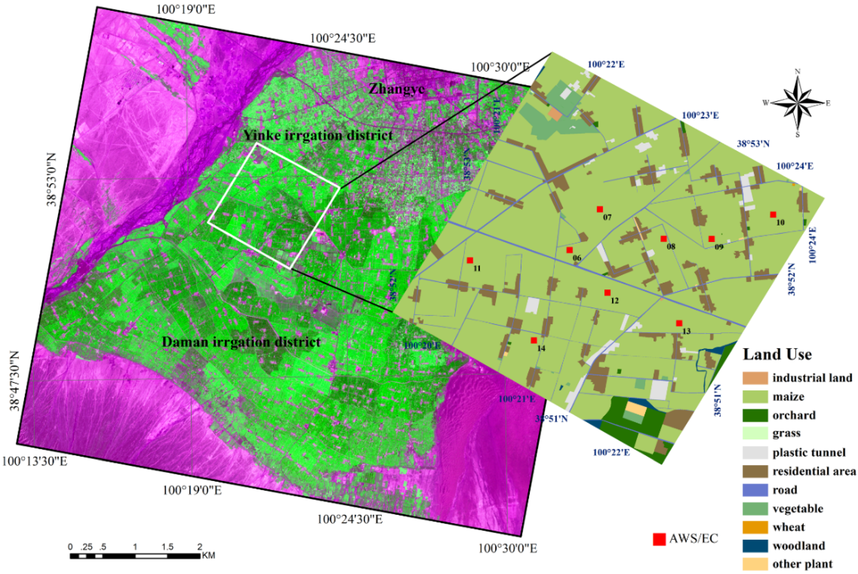
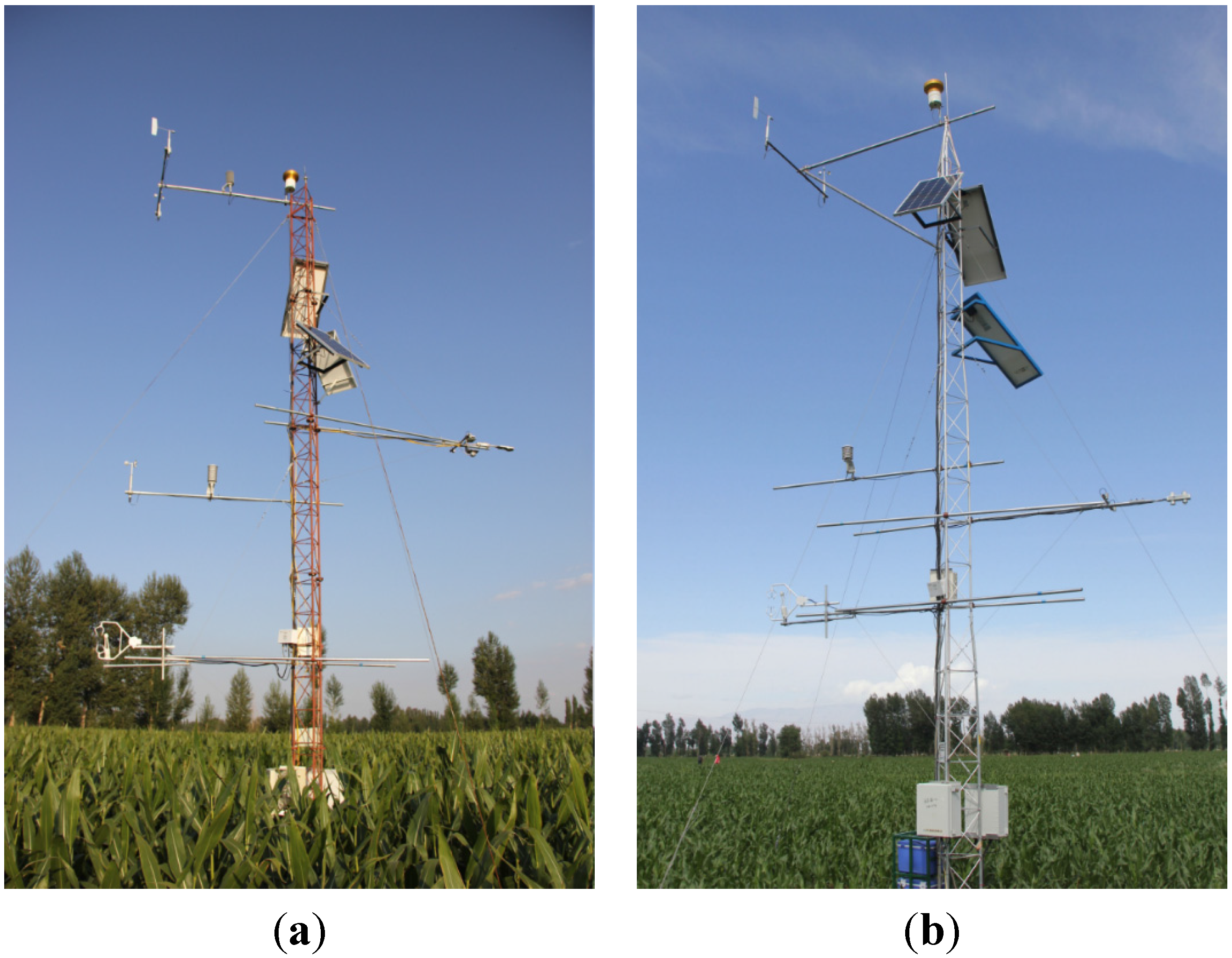
2.1. Study Site and Measurements


2.2. Remote Sensing Data
2.3. Methods
3. Results and Discussion
3.1. Surface Radiometric Temperature

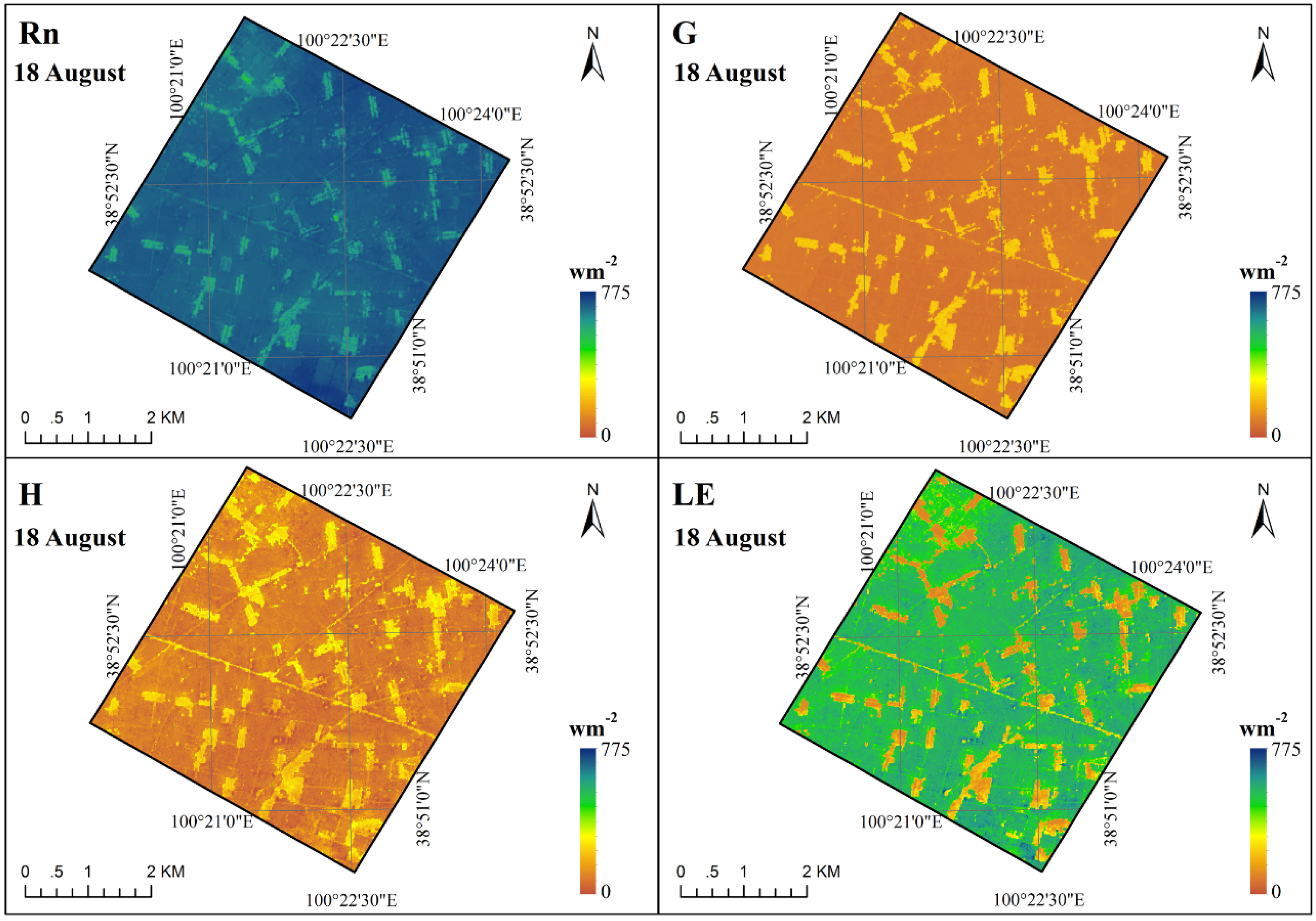
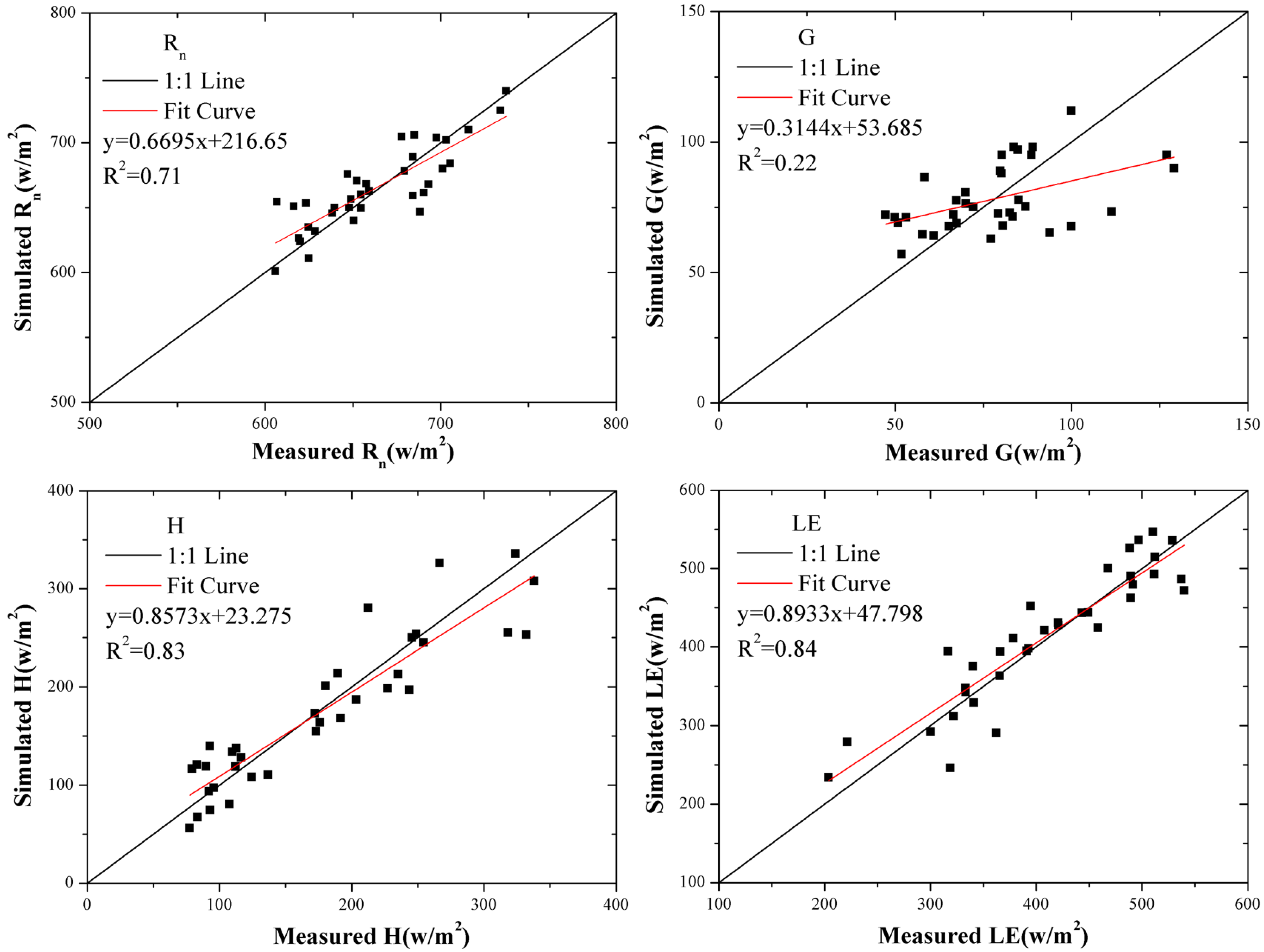
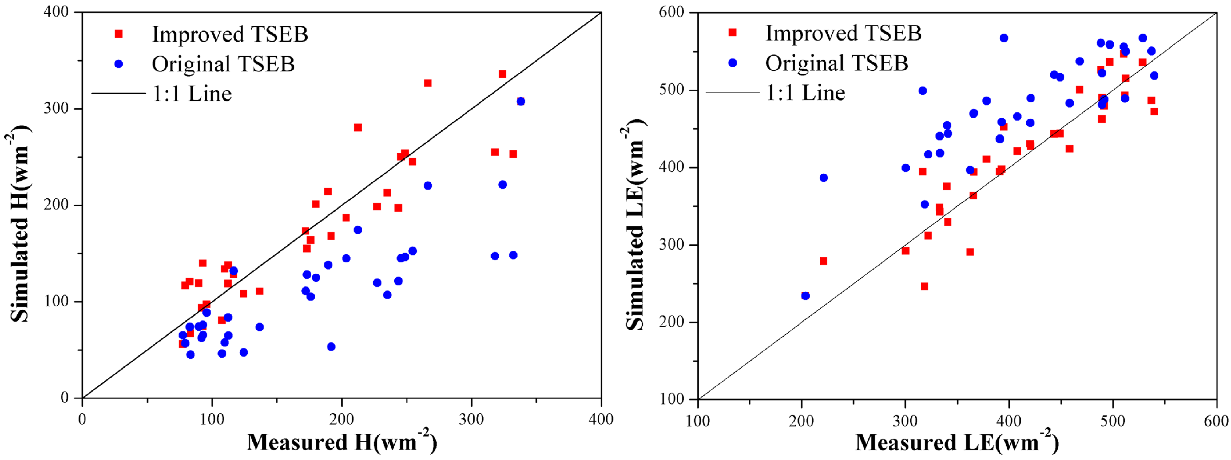
3.2. Instantaneous Surface Energy Fluxes


| Flux | Day | Observation Number | Observed Averaged (W·m−2) | Simulated Averaged (W·m−2) | Bias (W·m−2) | RMSD (W·m−2) | MAPD (%) |
|---|---|---|---|---|---|---|---|
| Rn | 11 August | 8 | 653.4 | 661.0 | 7.6 | 22.1 | 2.8 |
| 18 August | 9 | 671.3 | 675.7 | 4.4 | 15.1 | 1.9 | |
| 3 September | 9 | 666.4 | 662.2 | −4.2 | 26.3 | 3.3 | |
| 12 September | 9 | 659.1 | 660.8 | 1.7 | 6.9 | 0.9 | |
| Overall | 35 | 662.5 | 664.9 | 2.4 | 19.0 | 2.2 | |
| G | 11 August | 8 | 80.0 | 77.7 | −2.3 | 17.8 | 17.1 |
| 18 August | 9 | 75.2 | 75.1 | −0.1 | 16.7 | 20.7 | |
| 3 September | 9 | 80.2 | 77.3 | −2.9 | 23.5 | 25.9 | |
| 12 September | 9 | 74.6 | 79.5 | 4.9 | 7.1 | 8.6 | |
| Overall | 35 | 77.5 | 77.4 | −0.1 | 17.3 | 18.1 | |
| H | 11 August | 8 | 111.5 | 116.6 | 5.1 | 27.0 | 25.8 |
| 18 August | 9 | 100.7 | 104.1 | 3.4 | 22.8 | 18.7 | |
| 3 September | 9 | 200.1 | 189.1 | −11.0 | 24.3 | 10.2 | |
| 12 September | 9 | 282.3 | 278.5 | −3.8 | 46.8 | 13.2 | |
| Overall | 35 | 173.7 | 172.1 | −1.6 | 31.9 | 16.7 | |
| LE | 11 August | 8 | 461.9 | 466.7 | 4.8 | 38.2 | 6.4 |
| 18 August | 9 | 495.3 | 496.4 | 1.1 | 25.0 | 3.9 | |
| 3 September | 9 | 386.1 | 395.9 | 9.8 | 22.2 | 4.7 | |
| 12 September | 9 | 302.2 | 302.8 | 0.6 | 48.6 | 13.5 | |
| Overall | 35 | 411.4 | 415.5 | 4.1 | 35.1 | 7.1 |


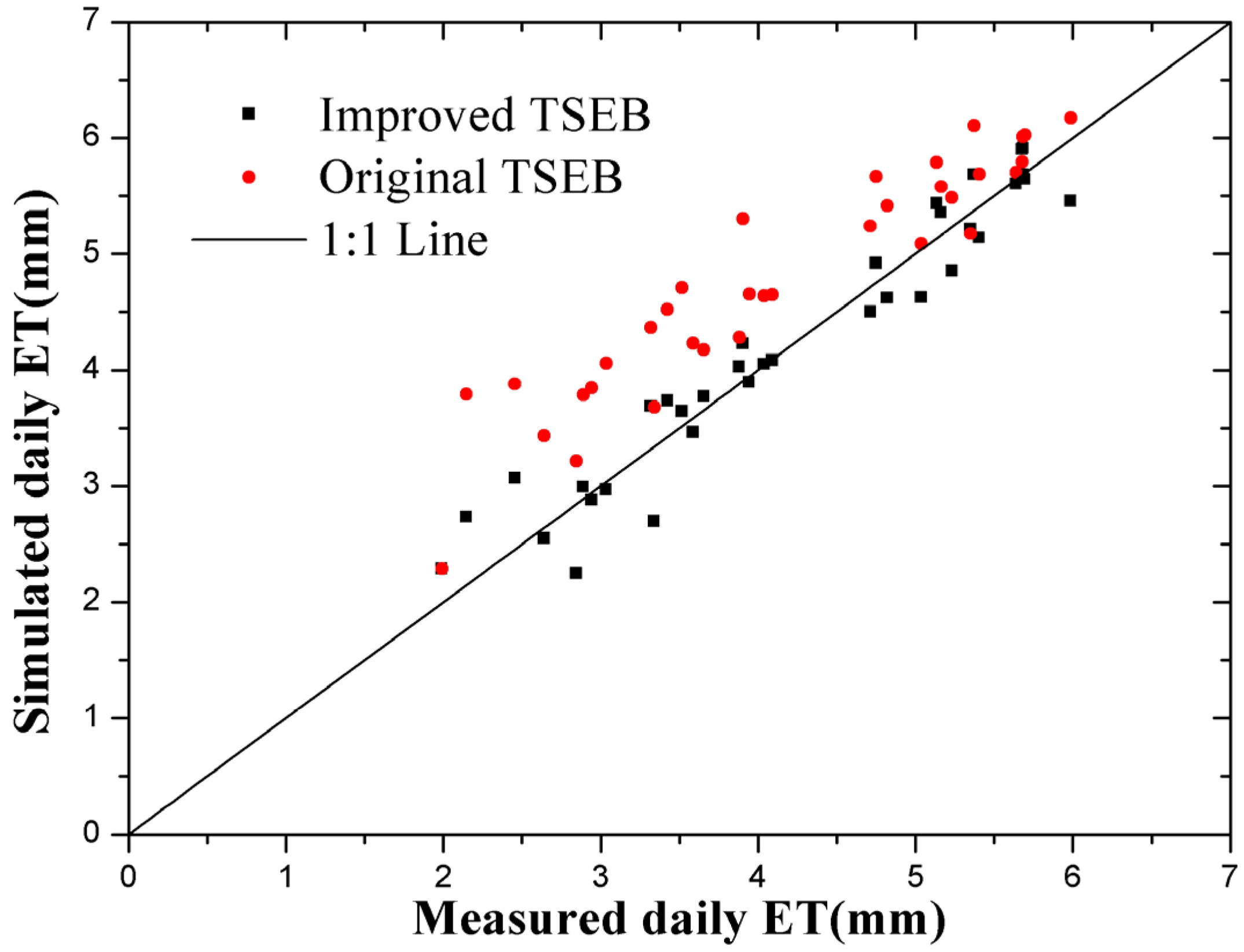
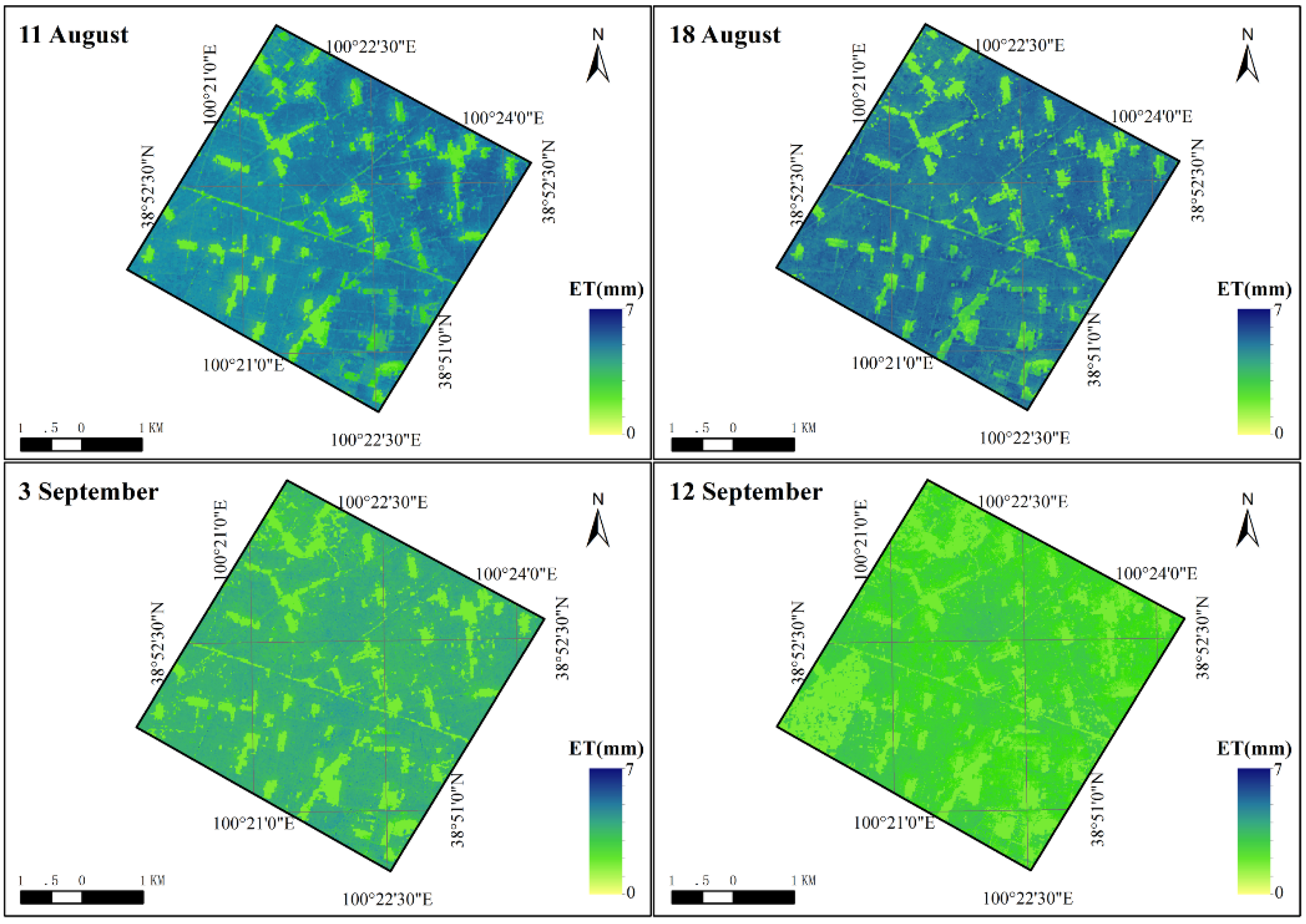
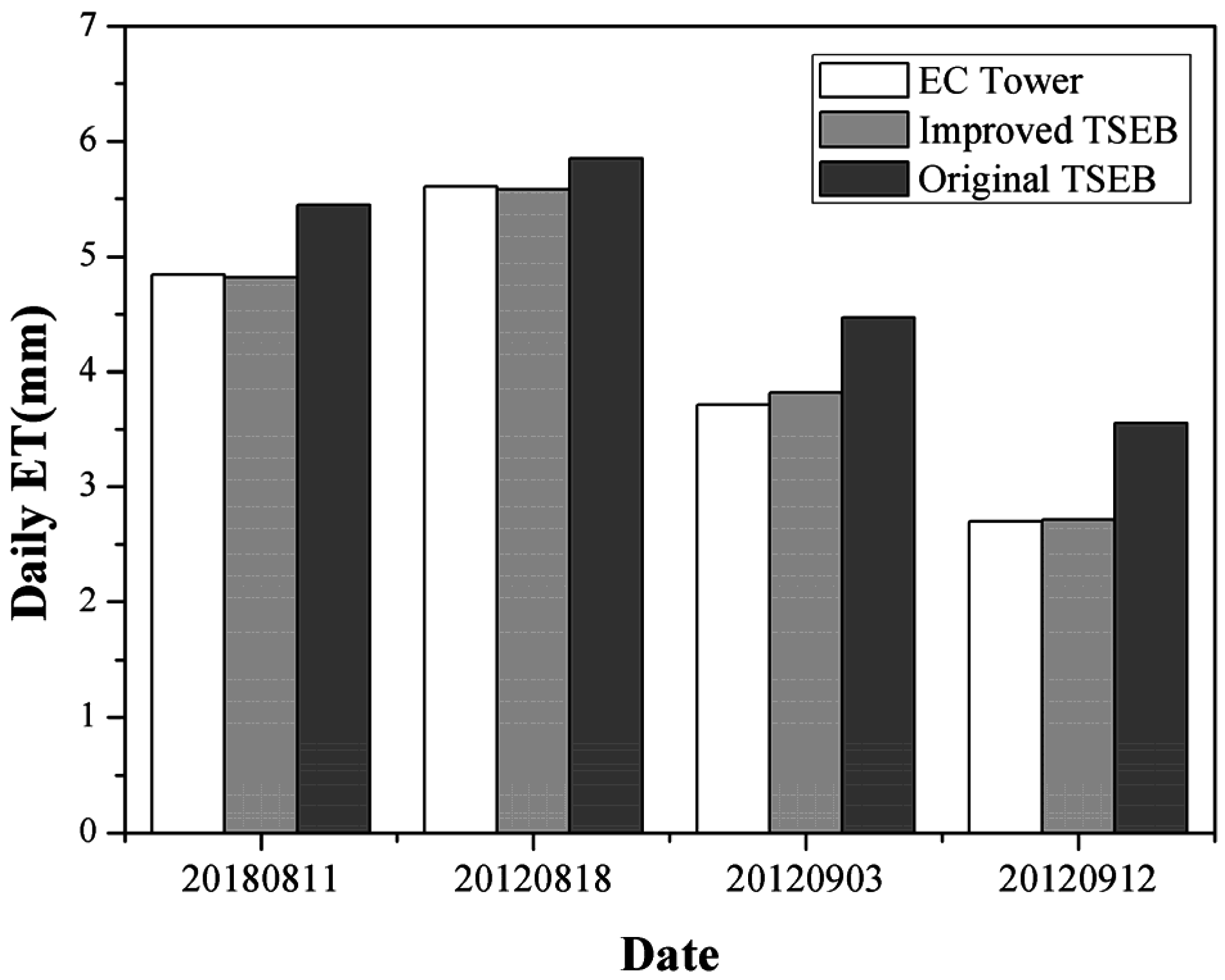
3.3. Daily ET


| Model | RMSD (mm) | BIAS (mm) | MAPD (%) |
|---|---|---|---|
| Improved TSEB | 0.30 | 0.02 | 6.63 |
| Original TSEB | 0.74 | 0.61 | 18.16 |
3.4. Determination of the Effects of Plant Constraints
| Date | fg | fm | ft |
|---|---|---|---|
| 11 August | 0.96 | 0.72 | 1.00 |
| 18 August | 0.98 | 0.82 | 0.99 |
| 3 September | 0.95 | 0.70 | 0.81 |
| 12 September | 0.88 | 0.51 | 0.52 |
| Flux | Day | Observed Averaged (W·m−2) | Improved TSEB Averaged (W·m−2) | Original TSEB Averaged (W·m−2) | TSEB (αpt = 1.1) Averaged (W·m−2) |
|---|---|---|---|---|---|
| H | 11 August | 111.5 | 116.6 | 55.6 | 78.1 |
| 18 August | 100.7 | 104.1 | 80.1 | 94.9 | |
| 3 September | 200.1 | 189.1 | 122.2 | 141.9 | |
| 12 September | 282.3 | 278.5 | 184.8 | 199.4 | |
| LE | 11 August | 461.9 | 466.7 | 527.7 | 505.2 |
| 18 August | 495.3 | 496.4 | 520.5 | 505.7 | |
| 3 September | 386.1 | 395.9 | 462.8 | 443.0 | |
| 12 September | 302.2 | 302.8 | 396.6 | 381.9 |
4. Conclusions
Acknowledgments
Author Contributions
Conflicts of Interest
References
- Merlin, O.; Chirouze, J.; Olioso, A.; Jarlan, L.; Chehbouni, G.; Boulet, G. An image-based four-source surface energy balance model to estimate crop evapotranspiration from solar reflectance/thermal emission data (SEB-4S). Agric. For. Meteorol. 2014, 184, 188–203. [Google Scholar] [CrossRef] [Green Version]
- Bastiaanssen, W.G.M.; Menenti, M.; Feddes, R.A.; Holtslag, A.A.M. A remote sensing surface energy balance algorithm for land (SEBAL): 1. Formulation. J. Hydrol. 1998, 212–213, 198–212. [Google Scholar] [CrossRef]
- Allen, R.G.; Tasumi, M.; Trezza, R. Satellite-based energy balance for mapping evapotranspiration with internalized calibration (METRIC)-model. J. Irrig. Drain. Eng. 2007, 133, 380–394. [Google Scholar] [CrossRef]
- Su, Z. The surface energy balance system (SEBS) for estimation of turbulent heat fluxes. Hydrol. Earth Syst. Sci. 2002, 6, 85–99. [Google Scholar] [CrossRef]
- Norman, J.M.; Kustas, W.P.; Humes, K.S. Source approach for estimating soil and vegetation energy fluxes in observations of directional radiometric surface temperature. Agric. For. Meteorol. 1995, 77, 263–293. [Google Scholar] [CrossRef]
- Gokmen, M.; Vekerdy, Z.; Verhoef, A.; Verhoef, W.; Batelaan, O.; van der Tol, C. Integration of soil moisture in SEBS for improving evapotranspiration estimation under water stress conditions. Remote Sens. Environ. 2012, 121, 261–274. [Google Scholar] [CrossRef]
- Paul, G.; Gowda, P.H.; Prasad, P.V.V.; Howell, T.A.; Aiken, R.M.; Neale, C.M.U. Investigating the influence of roughness length for heat transport (zoh) on the performance of SEBAL in semi-arid irrigated and dryland agricultural systems. J. Hydrol. 2014, 509, 231–244. [Google Scholar] [CrossRef]
- Lhomme, J.P.; Chehbouni, A. Comments on dual-source vegetation-atmosphere transfer models. Agric. For. Meteorol. 1999, 94, 269–273. [Google Scholar] [CrossRef]
- Sanchez, J.M.; Kustas, W.P.; Caselles, V.; Anderson, M. Modelling surface energy fluxes over maize using a two-source patch model and radiometric soil and canopy temperature observations. Remote Sens. Environ. 2008, 112, 1130–1143. [Google Scholar] [CrossRef]
- Anderson, M.C.; Norman, J.M.; Kustas, W.P.; Houborg, R.; Starks, P.J.; Agam, N. A thermal-based remote sensing technique for routine mapping of land-surface carbon, water and energy fluxes from field to regional scales. Remote Sens. Environ. 2008, 112, 4227–4241. [Google Scholar] [CrossRef]
- Long, D.; Singh, V.P. A Two-source Trapezoid Model for Evapotranspiration (TTME) from satellite imagery. Remote Sens. Environ. 2012, 121, 370–388. [Google Scholar] [CrossRef]
- Kustas, W.P.; Norman, J.M. A two-source approach for estimating turbulent fluxes using multiple angle thermal infrared observations. Water Resour. Res. 1997, 33, 1495–1508. [Google Scholar] [CrossRef]
- Morillas, L.M.; Villagarcia, L.; Domingo, F.; Nieto, H.; Ucles, O.; Garcia, M. Environmental factors affecting the accuracy of surface fluxes from a two-source model in Mediterranean drylands: Upscaling instantaneous to daytime estimates. Agric. For. Meteorol. 2014, 189–190, 140–158. [Google Scholar] [CrossRef]
- Li, F.Q.; Kustas, W.P.; Prueger, J.H.; Neale, C.M.U.; Jackson, T.J. Utility of remote sensing-based two-source energy balance model under low- and high-vegetation cover conditions. J. Hydrometeorol. 2005, 6, 878–891. [Google Scholar] [CrossRef]
- Gonzalez-Dugo, M.P.; Neale, C.M.U.; Mateos, L.; Kustas, W.P.; Prueger, J.H.; Anderson, M.C.; Li, F. A comparison of operational remote sensing-based models for estimating crop evapotranspiration. Agric. For. Meteorol. 2009, 149, 1843–1853. [Google Scholar] [CrossRef]
- Consoli, S.; Vanella, D. Comparisons of satellite-based models for estimating evapotranspiration fluxes. J. Hydrol. 2014, 513, 475–489. [Google Scholar] [CrossRef]
- Liu, S.M.; Xu, Z.W.; Zhu, Z.L.; Jia, Z.Z.; Zhu, M.J. Measurements of evapotranspiration from eddy-covariance systems and large aperture scintillometers in the Hai River Basin, China. J. Hydrol. 2013, 487, 24–38. [Google Scholar] [CrossRef]
- Twine, T.E.; Kustas, W.P.; Norman, J.M.; Cook, D.R.; Houser, P.R.; Meyers, T.P.; Prueger, J.H.; Starks, P.J.; Wesely, M.L. Correcting eddy-covariance flux underestimates over a grassland. Agric. For. Meteorol. 2000, 103, 279–300. [Google Scholar] [CrossRef]
- Wang, Y.Y.; Li, X.X.; Tang, S.H. Validation of the SEBS-derived sensible heat for FY3A/VIRR and TERRA/MODIS over an alpine grass region using LAS measurements. Int. J. Appl. Earth Obs. 2013, 23, 226–233. [Google Scholar] [CrossRef]
- Jimenez-Munoz, J.C.; Sobrino, J.A. Feasibility of retrieving land-surface temperature from ASTER TIR bands using two-channel algorithms: A case study of agricultural areas. IEEE Geosci. Remote Sens. Lett. 2007, 4, 60–64. [Google Scholar] [CrossRef]
- Kustas, W.; Norman, J.; Anderson, M.; French, A. Estimating subpixel surface temperatures and energy fluxes from the vegetation index-radiometric temperature relationship. Remote Sens. Environ. 2003, 85, 429–440. [Google Scholar] [CrossRef]
- Mira, M.; Valor, E.; Boluda, R.; Caselles, V.; Coll, C. Influence of soil water content on the thermal infrared emissivity of bare soils: Implication for land surface temperature determination. J. Geophys. Res. 2007, 112. [Google Scholar] [CrossRef]
- Rubio, E.; Caselles, V.; Coll, C.; Valour, E.; Sospedra, F. Thermal-infrared emissivities of natural surfaces: Improvements on the experimental set-up and new measurements. Int. J. Remote Sens. 2003, 24, 5379–5390. [Google Scholar] [CrossRef]
- Consoli, S.; D’Urso, G.; Toscano, A. Remote sensing to eatimate ET-fluxes and the performance of an irrigation district in southern Italy. Agric. Water Manag. 2006, 81, 295–314. [Google Scholar] [CrossRef]
- Colaizzi, P.D.; Kustas, W.P.; Anderson, M.C.; Agam, N.; Tolk, J.A.; Evett, S.R.; Howell, T.A.; Gowda, P.H.; O’Shaughnessy, S.A. Two-source energy balance model estimates of evapotranspiration using component and composite surface temperatures. Adv. Water Resour. 2012, 50, 134–151. [Google Scholar] [CrossRef]
- Norman, J.M.; Kustas, W.P.; Prueger, J.H.; Diak, G.R. Surface flux estimation using radiometric temperature: A dual-temperature-difference method to minimize measurement errors. Water Resour. Res. 2000, 36, 2263–2274. [Google Scholar] [CrossRef]
- Fisher, J.B.; Tu, K.P.; Baldocchi, D.D. Global estimates of the land–atmosphere water flux based on monthly AVHRR and ISLSCP-II data, validated at 16 FLUXNET sites. Remote Sens. Environ. 2013, 112, 901–919. [Google Scholar] [CrossRef]
- Garcia, M.; Sandholt, I.; Ceccato, P.; Ridler, M.; Mougin, E.; Kergoat, L.; Morillsa, L.; Timouk, F.; Fensholt, R.; Domingo, F. Actual evapotranspiration in drylands derived from in situ and satellite data: Assessing biophysical constraints. Remote Sens. Environ. 2013, 131, 103–118. [Google Scholar] [CrossRef]
- Myneni, R.B.; Williams, D.L. On the relationship between FAPAR and NDVI. Remote Sens. Environ. 1994, 49, 200–211. [Google Scholar] [CrossRef]
- Yuan, W.P.; Liu, S.G.; Yu, G.R.; Bonnefond, J.M.; Chen, J.Q.; Davis, K.; Desai, A.R.; Goldstein, A.H.; Gianelle, D.; Rossi, F.; et al. Global estimates of evapotranspiration and gross primary production based on MODIS and global meteorology data. Remote Sens. Environ. 2010, 114, 1416–1431. [Google Scholar] [CrossRef]
- Choi, M.; Kustas, W.P.; Anderson, M.C.; Allen, R.G.; Li, F.Q.; Kjaersgaard, J.H. An intercomparison of three remote sensing-based surface energy balance algorithms over a corn and soybean production region (Iowa, US) during SMACEX. Agric. For. Meteorol. 2009, 149, 2082–2097. [Google Scholar] [CrossRef]
- Guzinski, R.; Anderson, M.C.; Kustas, W.P.; Nieto, H.; Sandholt, I. Using a thermal-based two source energy balance model with time-differencing to estimate surface energy fluxs with day-night MODIS observations. Hydrol. Earth Syst. Sci. 2013, 17, 2809–2825. [Google Scholar] [CrossRef]
© 2015 by the authors; licensee MDPI, Basel, Switzerland. This article is an open access article distributed under the terms and conditions of the Creative Commons by Attribution (CC-BY) license (http://creativecommons.org/licenses/by/4.0/).
Share and Cite
Zhuang, Q.; Wu, B. Estimating Evapotranspiration from an Improved Two-Source Energy Balance Model Using ASTER Satellite Imagery. Water 2015, 7, 6673-6688. https://doi.org/10.3390/w7126653
Zhuang Q, Wu B. Estimating Evapotranspiration from an Improved Two-Source Energy Balance Model Using ASTER Satellite Imagery. Water. 2015; 7(12):6673-6688. https://doi.org/10.3390/w7126653
Chicago/Turabian StyleZhuang, Qifeng, and Bingfang Wu. 2015. "Estimating Evapotranspiration from an Improved Two-Source Energy Balance Model Using ASTER Satellite Imagery" Water 7, no. 12: 6673-6688. https://doi.org/10.3390/w7126653