Application of the Entropy Method to Select Calibration Sites for Hydrological Modeling

Abstract

Selecting an optimum number of calibration sites for hydrological modeling is challenging. Modelers often spend a lot of time and effort on trial and error because there is no guide. We propose a novel entropy method to automate the selection of the optimum combination of calibration sites. To illustrate, the proposed entropy method is applied using discharge data from one river basin in Korea. First, different combinations of discharge-gauging sites were grouped based on the maximum information estimated by the entropy method. Then, a hydrological model was set up for the study basin and was calibrated by estimating optimal parameters using a genetic algorithm at the discharge-gauging sites. The calibration result confirmed that the model’s performance was best when it was calibrated using the site number and combination suggested by the entropy method. In addition, the entropy method was useful in reducing the time and effort of model calibration. Therefore, we suggest and confirm the applicability of the entropy method in selecting calibration sites for hydrological modeling.

1. Introduction

Hydrological models are increasingly used to evaluate the impacts of climate, land use, and crop management practices on the quantity of water resources [1]. The two main objectives of hydrological modeling are to explore the implications of making certain assumptions about the nature of the real-world system and to predict the system’s behavior under a set of naturally occurring circumstances [2]. The successful application of any hydrological model is dependent on the quality of its calibration [3]. As a result, developing calibration strategies is a requirement for their proper application in hydrological modeling. During the calibration process, model parameters are estimated by minimizing the deviation between the measured and simulated discharges. Researchers have suggested a number of methodologies to improve calibration-related issues [4,5,6,7,8,9,10,11].

Over the past decades, information technologies, such as the Geographical Information System (GIS), have developed significantly and several GIS-based hydrological models have been created. The GIS provides spatial data as inputs for the variables needed in hydrological models. The GIS has contributed to the change in hydrology from simplified conceptual models to high-resolution distributed models. Runoff analysis, using a physically-based distributed model, gains an advantage from its ability to reflect the spatial characteristics of a watershed’s physical parameters [12]. The parameters in a physically-based distributed model are classified as those set up through observation and those set up through estimation. Ideally, parameters established through observation should not require calibration; however, because of scale problems and observation errors, it is still required [4,13,14,15,16,17]. As the parameters are dependent on the topography, land cover and soil characteristics are allocated by a grid or a sub-basin. There have also been many studies about real-life case studies of soft computing techniques in hydrologic engineering [18,19,20,21,22,23,24].

Until now, the calibration of the hydrological model has focused on estimating the optimum parameters. The traditional approach to calibrating hydrological models has relied on a single objective function, such as Root-Mean-Square Error (RMSE) or Percent Bias, among others [25]. Local search methods, such as the simplex method [26], have a very low probability of success in finding the global optimum parameter set [3]. Currently available global search methods are the population-evolution-based Shuffled Complex Evolution-University of Arizona (SCE-UA) [3] and Genetic Algorithms (GA) [27]. Other studies have also been conducted on the selection of calibration sites. When runoff is calculated at multiple sites in a watershed, the most intuitive method to guarantee the physical and hydrological similarities between the watershed where the model is calibrated and the sub-basin where the model will be simulated is to calibrate the model using the stream gauges near the sub-basin outlet [15,28,29,30,31]. Choi, et al. [31] and Zhang, et al. [32] suggested the importance of calibration at multiple sites in the basin.

Recently, many discharge-gauging stations have been installed in basins to manage water resources, such as forecasting and issuing warnings for possible flooding events. When establishing and calibrating the hydrological model, the issue of selecting sites naturally arises. Of course, to select discharge-gauging sites, the spatial resolution can be considered, depending on the purpose of establishing the hydrological model and the quality or the importance of the discharge-gauging sites. However, there is no generalized guide for this even though there have been a significant number of studies as the above references, and it depends on the modeler’s experience. Sometimes we do not have confidence in the calibrated results even though we spend a large amount of time and effort. The aim of this study under the problems is to confirm the applicability of the entropy method when selecting observation sites to calibrate the hydrological model in multiple sites. The basic theory of the application methodology, including the entropy method, is introduced in Section 2. Section 3 is an analysis and discussion of the application and the results of the methodology for the study basin, and Section 4 consists of the study’s conclusion.

2. Methodology and Basic Theory

In this study, the procedure and methodology, as seen in Figure 1, were constructed to review and confirm the entropy method’s applicability when selecting the calibration sites of the hydrological model. Data were collected at the discharge-gauging sites within the study basin, and discharge-gauging sites were combined based on the number of sites with maximum information. Then, the Soil and Water Assessment Tool (SWAT) was established for the study basin, and the entropy method was used to calibrate the model at the selected sites. GA was used to optimize the parameters for each site. Finally, the model was calibrated using the site combination with maximum information, depending on the selected number of sites, and the result was evaluated.

Figure 1. A schematic drawing of the analysis procedure.

Figure 1. A schematic drawing of the analysis procedure.

2.1. Entropy Method for Information Measurement

Shannon and Weaver [33] defined the marginal entropy for the discrete random variable, shown in Equation (1):

$$H\left(X\right)=-{\displaystyle \sum }_{n=1}^{N}p\left(x_n\right)\text{ln }p\left(x_n\right),n=1,2,3,\cdots ,N$$

(1)

where $p\left(x_n\right)$ is the occurrence probability of $x_n$. The marginal entropy $H\left(X\right)$ is the amount of information (or uncertainty) of $X$.

If there exists $y_m\left(m=1,2,\cdots ,N\right)$ related to a random variable $x_n$, it may be possible to reduce the uncertainty of $x_n$ by using $y_m$ to estimate $x_n$. Using this principle, the remaining uncertainty in $X$ with the given $Y$ can be estimated, as shown in Equation (2):

$$H\left(X|Y\right)=-{\displaystyle \sum }_{n=1}^N{\displaystyle \sum }_{m=1}^{N}p\left(x_n,y_m\right)\text{ln }p\left(x_n|y_m\right)$$

(2)

where $p\left({\text{x}}_{\text{n}},y_m\right)$ is the joint probability of $X=\left\{x_n\right\}$ and $Y=\left\{y_m\right\}$, and $p\left(x_n|y_m\right)$ is the conditional probability of $X$ with the given $Y$. $H\left(X|Y\right)$ is then the conditional entropy of $X$ with the given $Y$, which can also be interpreted as the information loss in the transinformation between $X$ and $Y$ [34]. The reduction of uncertainty in $X$ with the given $Y$, or the transinformation between $X$ and $Y$, is defined in Equation (3):

$$T\left(X,Y\right)=H\left(X\right)-H\left(X|Y\right)$$

(3)

This concept of entropy can be applied to the analysis of a hydrological time series. In this study, the variable X is defined as the daily stream flow. It is assumed that X is a continuous random variable with a probability density function f(x).

If the range of $X$ is divided by the class interval $∆x$, then the marginal entropy $X$ can be computed with Equation (4):

$$H\left(X;∆x\right)\simeq -\underset{0}{\overset{\infty }{{\displaystyle \int }}}f\left(x\right)\text{ln}f\left(x\right)\text{d}x-\text{ln}∆x$$

(4)

Moreover, if the same class interval $∆x$ is applied for $Y$, then the conditional entropy of $X$ with the given $Y$ can be computed with Equation (5):

$$H\left(X|Y;∆x\right)\simeq -\underset{0}{\overset{\infty }{{\displaystyle \int }}}\underset{0}{\overset{\infty }{{\displaystyle \int }}}f\left(x,y\right)\text{ln}f\left(x|y\right)\text{d}x\text{d}y-\text{ln}∆x$$

(5)

when $X$ and $Y$ follow the log-normal distribution function, the marginal entropy, the conditional entropy, and the transinformation are derived, respectively, in Equations (6)–(8) [35]:

$$H\left(X;∆x\right)={\text{μ}}_{\text{z}}+0.5\text{ln}(2{\text{πeσ}}_{\text{z}}^2)-\text{ln}∆x$$

(6)

$$H\left(X|Y;∆x\right)={\text{μ}}_{\text{z}}+0.5\left[\text{ln}(2{\text{πeσ}}_{\text{z}}^2\right)\left(1-{\text{ρ}}_{\text{zω}}^2\right)]-\text{ln}∆x$$

(7)

$$T\left(X,Y\right)=-0.5\text{ln}\left(1-{\text{ρ}}_{\text{zω}}^2\right)$$

(8)

where ${\text{μ}}_{\text{z}}$ and ${\text{σ}}_z$ are the mean and the standard deviation of $z=(\text{ln }x)$, respectively, and ${\text{ρ}}_{\text{zw}}$ represents the cross-correlation coefficient between $\text{z}$ and $\text{ω}(=\text{ln }y)$. Chapman [36] also derived the marginal entropy and the conditional entropy, like in Equations (9) and (10), while considering the varying interval $∆x/x$ to be proportional to the range instead of being a fixed class interva$∆x$. The transinformation $T\left(X,Y\right)$ between $X$ and $Y$ is independent of the class interval from Equation (8).

$$H\left(X;∆x/x\right)=0.5\text{ln}(2{\text{πeσ}}_{\text{z}}^2)-\text{ln}\left(∆x/x\right)$$

(9)

$$H\left(X|Y;∆x/x\right)=0.5\left[\text{ln}(2{\text{πeσ}}_{\text{z}}^2\right)\left(1-{\text{ρ}}_{\text{zω}}^2\right)]-\text{ln}\left(∆x/x\right)$$

(10)

The decision problem in calibration for hydrological modeling minimizes the redundant information and maximizes the total information from the selected discharge-gauging sites. Thus, the objective function of this optimization problem can be formulated as shown in Equation (11) [37,38]:

$${\text{MAXI}}_{\text{Total}}\left(X_1,X_2,\cdots ,X_m;X_i,X_{ii},\cdots ,X_k\right)$$

(11)

where $\text{m}$ is the total number of discharge-gauging sites operating in the basin and $\text{k}$ is the number of discharge-gauging sites selected of the m discharge-gauging sites. A set of $\text{k}$ sites $i,ii,\cdots ,k)$ is selected to maximize the total information, $I_{\text{Total}}\left(X_1,X_2,\cdots ,X_m;X_i,X_{ii},\cdots ,X_k\right)$. Equation (11) can also be expressed as follows in Equation (12):

$$\text{MAX}{I}_{\text{Total}}=\text{ MAX}\left[H\left(X_i\right)+H\left(X_{ii}\right)+\cdots +H\left(X_k\right)+{\displaystyle \sum }_{x=1}^{m-k}{\displaystyle \sum }_{y=\text{i}}^{k}T\left(X_x,X_y\right)\right], x\ne y$$

(12)

where $H\left(X_i\right)+H\left(X_{ii}\right)+\cdots +H\left(X_k\right)$ is the sum of the marginal entropy from the selected discharge-gauging sites, and $\sum _{x=1}^{m-k}\sum _{y=i}^k\text{T}\left(X_x,X_y\right)$ is the sum of transinformation between the selected and the unselected discharge-gauging sites. As the number of selected discharge-gauging sites increases, the total information obtained increases, but then decreases after hitting a threshold number of discharge-gauging sites. That is, the marginal entropy increases as the number of discharge-gauging sites increases, while the sum of transinformation decreases.

2.2. Genetic Algorithm

GA is an algorithm based on Charles Darwin’s “Survival of the Fittest” theory, the most widely known evolutionary theory. GA was first proposed by Holland [39] as a search algorithm that applied the natural selection of organisms to the mechanical learning area. GA has been applied to various application fields, such as pattern recognition, including optimization, machine learning, robot engineering, and TSP, the traveling salesman problem. GA is an organic evolution model in the natural world. It is a stochastic optimization method with excellent applicability in the real world that simulates the process where, among a group of individuals forming a generation, individuals with high environmental adaptability are more likely to survive (survival of the fittest), go through crossover and mutation, and form the next generation. In hydrology, GA was used as a methodology to overcome the local optimization of parameters in the main [40,41,42].

2.3. SWAT for Runoff Simulation

Numerous hydrological models have been developed to assist in understanding watershed system, such as MIKE-SHE (MIKE Système Hydrologique Européen) [43], Petroleum Resources Management System (PRMS) [44], SLURP (Semi-distributed Land Use-based Runoff Processes) [45], SWAT [46] and so on. Among the models, SWAT has been successfully applied in a wide variety of data-limited studies, particularly in South Korea [47]. SWAT as open-source software has an advantage to estimate parameters with an optimization tool like GA.

SWAT is a physically based and distributed agro-hydrological model that operates on a daily time step (as a minimum) at the watershed scale. It is designed to predict the impact of management on water, sediments, and agricultural chemical yields in ungauged catchments [46]. The model is capable of continuous simulation of dissolved and particulate elements in large complex catchments with varying weather, soils, and management conditions over long periods. SWAT can analyze small or large catchments by discretizing them into sub-basins, which are then further subdivided into hydrological response units with homogeneous land use, soil type, and slope. When embedded within a GIS, SWAT can integrate various spatial environmental data including soil, land cover, climate, and topographical features. The theory and details of the hydrological and sediment transport processes integrated in SWAT are available online in the SWAT documentation (http://swatmodel.tamu.edu/).

3. Application and Results

3.1. Study Area

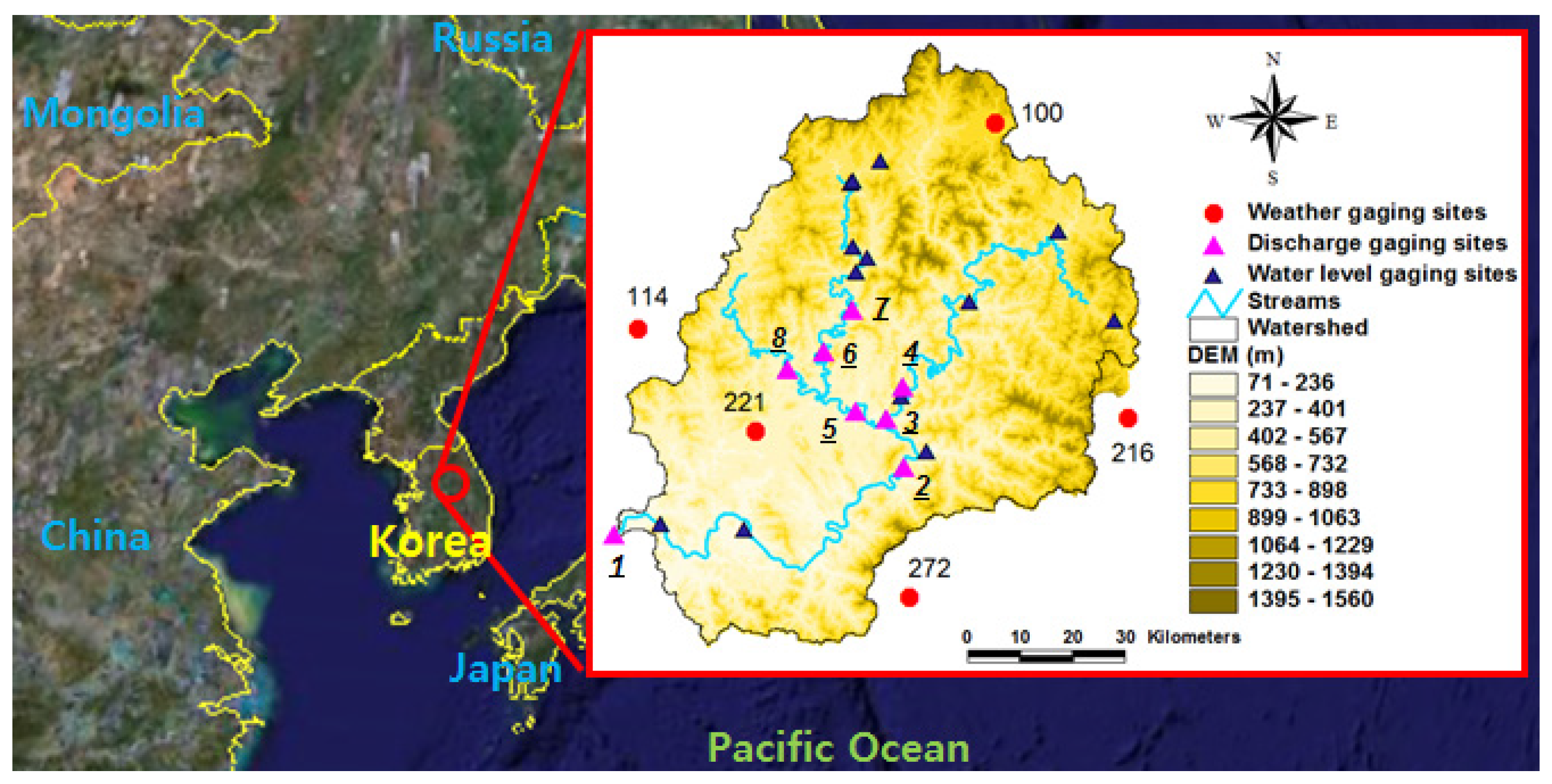
The study area was the Chungju Dam Basin in the Han River of the Korean peninsula. The area of the basin is approximately 6648 km², and the length of the related river is approximately 280 km. The average altitude of the basin, calculated using a 50 × 50 m² grid, is 610 m; its maximum altitude is 1560 m; its minimum altitude is 71 m; and its standard deviation is 261 m. We selected five weather-gauging sites (the red circles in Figure 2), which have collected data for five years (2008–2012), from the Korean Meteorological Agency. Table 1 shows the geographic information for the weather stations and the daily data (minimum temperature, maximum temperature, precipitation, relative humidity, wind speed, and solar radiation) from the collection period. There are 21 water-level gauging sites in the basin (the black and pink triangles in Figure 2). However, only eight discharge-gauging sites (the pink triangles in Figure 2) had discharge data for the period from 2008 to 2012, as most gauging stations were either recently installed or have not developed a relationship between water level and discharge.

Figure 2. Study area (Chungju Dam Basin).

Figure 2. Study area (Chungju Dam Basin).

Table 1. Weather and discharge-gauging stations.

Stations	Code	Station Name	Latitude (°)	Longitude (°)	Elevation (m)	Period of Record (Year)
Weather gauging stations	100	Daegoanrung	37.68	128.82	772.4	2008–2012
	114	Wonju	37.34	127.95	150.7	2008–2012
	216	Taebaek	37.17	128.99	714.2	2008–2012
	221	Jecheon	37.16	128.19	263.1	2008–2012
	272	Youngju	36.87	128.52	210.5	2008–2012
Discharge-gauging stations	1	Chungju Dam	37.00	128.00	80.0	2008–2012
	2	Youngchun	37.10	128.51	190.0	2008–2012
	3	Youngwol 1	37.18	128.48	200.0	2008–2012
	4	Geowun	37.23	128.51	221.0	2008–2012
	5	Youngwol 2	37.19	128.41	383.0	2008–2012
	6	Panwoon	37.30	128.38	722.0	2008–2012
	7	Pyeongchang	37.37	128.41	762.0	2008–2012
	8	Jucheon	37.27	128.27	720.0	2008–2012

Table 1. Weather and discharge-gauging stations.

Stations	Code	Station Name	Latitude (°)	Longitude (°)	Elevation (m)	Period of Record (Year)
Weather gauging stations	100	Daegoanrung	37.68	128.82	772.4	2008–2012
	114	Wonju	37.34	127.95	150.7	2008–2012
	216	Taebaek	37.17	128.99	714.2	2008–2012
	221	Jecheon	37.16	128.19	263.1	2008–2012
	272	Youngju	36.87	128.52	210.5	2008–2012
Discharge-gauging stations	1	Chungju Dam	37.00	128.00	80.0	2008–2012
	2	Youngchun	37.10	128.51	190.0	2008–2012
	3	Youngwol 1	37.18	128.48	200.0	2008–2012
	4	Geowun	37.23	128.51	221.0	2008–2012
	5	Youngwol 2	37.19	128.41	383.0	2008–2012
	6	Panwoon	37.30	128.38	722.0	2008–2012
	7	Pyeongchang	37.37	128.41	762.0	2008–2012
	8	Jucheon	37.27	128.27	720.0	2008–2012

3.2. Entropy Estimation

The concept of entropy has been applied to several fields of study, for example, Jaynes [48] in statistical mechanics, Molgedey and Ebeling [49] in finance, Ulanowicz [50] in ecology, Mormarco, et al. [51] in hydraulics, Mogheir, et al. [52] in groundwater, and others. In hydrology, entropy has mostly been applied as a tool for modeling and decision-making (Singh [53,54]) including the evaluation of a sampling network. Yoo, et al. 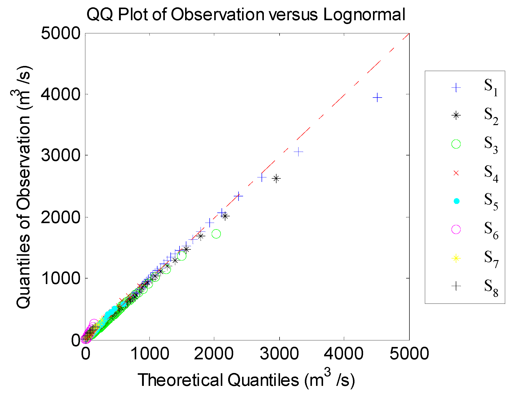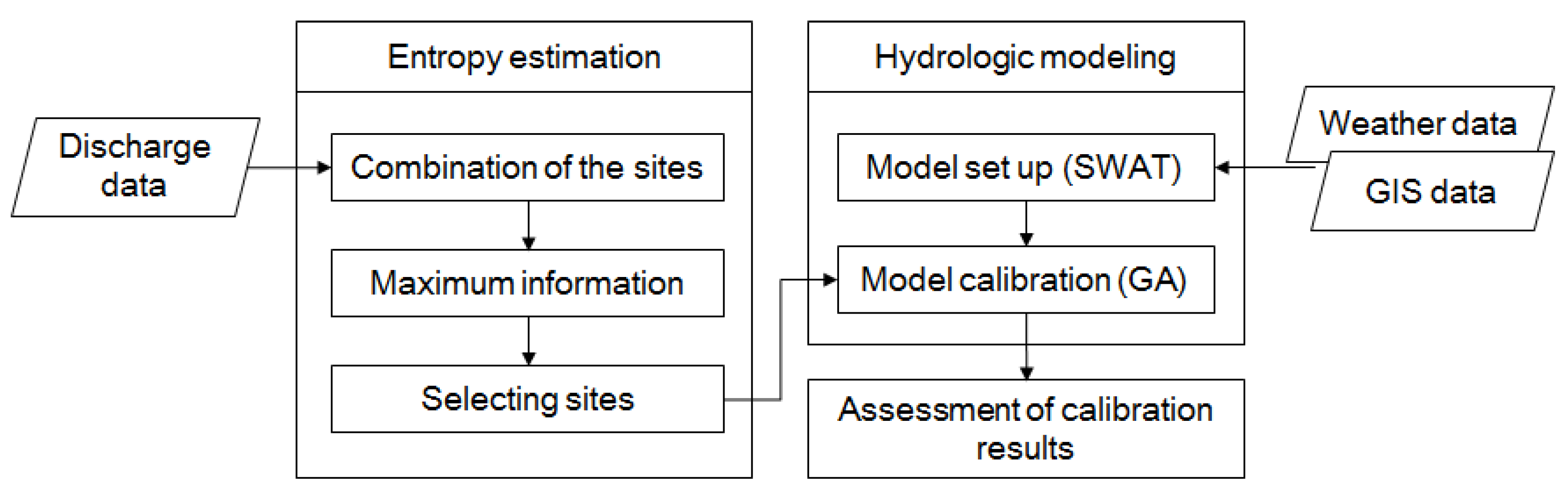[55] evaluated the rain gauge network by comparing mixed and continuous distribution function applications. This study tried to apply the entropy method to find calibration sites for hydrological modeling. In this study, the number of class intervals was set to 500 for all sites. Mutual information was calculated using the same class interval number, though the class intervals’ Δx are different from each site. First, the goodness-of-fit of the observed data for the log-normal distribution was tested. The Quantile-Quantile (QQ) plot, which is a very useful plot as one of several heuristics for assessing how closely a data set fits a particular distribution used to visually inspect the similarity between theoretical quantiles of log-normal distribution and quantiles of observation fit comparatively well in each site, as shown in Figure 3.

Figure 3. Quantile-Quantile (QQ) plot of observation versus log-normal distribution.

Figure 3. Quantile-Quantile (QQ) plot of observation versus log-normal distribution.

Table 2 shows the information matrices of the discharge-gauging sites from the entropy method. These matrices summarize the marginal entropy, transinformations between the sites, and the total information for a selected site, represented as the “sum”. For example, if we select Discharge-Gauging Site 1 in Table 2, the total information from Gauging Site 1 is the marginal entropy (7.667) plus the sum of the transinformations.

Table 3 summarizes the optimal sites depending on the total number of sites. At the beginning of the selection of the discharge-gauging sites, the sum of the marginal entropy of the selected sites and the transinformations with the other sites is increasing. The increasing trend is valid until the threshold number of sites for a given basin. However, after the threshold number of discharge-gauging sites, the sum of transinformation between the selected site and the other unselected sites decreases more rapidly than the additional marginal entropy from a newly selected site. The total entropy thus decreases as the number of selected sites increases. In the study area, the highest number of maximum information is 66 when the five sites (Sites 1, 2, 3, 5, and 6) are selected.

Table 2. Information matrix.

Discharge-Gauging Sites	Discharge-Gauging Sites
	1	2	3	4	5	6	7	8	Sum
1	7.667	2.708	2.643	2.543	2.353	1.745	2.128	1.609	23.396
2	2.708	7.079	2.599	2.530	2.337	1.452	2.070	1.641	22.415
3	2.643	2.599	6.783	2.505	2.771	1.867	2.354	1.857	23.378
4	2.543	2.530	2.505	6.007	2.755	2.049	2.462	1.948	22.798
5	2.353	2.337	2.771	2.755	6.457	1.938	2.353	1.808	22.772
6	1.745	1.452	1.867	2.049	1.938	4.288	3.075	2.474	18.888
7	2.128	2.070	2.354	2.462	2.353	3.075	5.124	2.187	21.755
8	1.609	1.641	1.857	1.948	1.808	2.474	2.187	4.140	17.665

Table 2. Information matrix.

Discharge-Gauging Sites	Discharge-Gauging Sites
	1	2	3	4	5	6	7	8	Sum
1	7.667	2.708	2.643	2.543	2.353	1.745	2.128	1.609	23.396
2	2.708	7.079	2.599	2.530	2.337	1.452	2.070	1.641	22.415
3	2.643	2.599	6.783	2.505	2.771	1.867	2.354	1.857	23.378
4	2.543	2.530	2.505	6.007	2.755	2.049	2.462	1.948	22.798
5	2.353	2.337	2.771	2.755	6.457	1.938	2.353	1.808	22.772
6	1.745	1.452	1.867	2.049	1.938	4.288	3.075	2.474	18.888
7	2.128	2.070	2.354	2.462	2.353	3.075	5.124	2.187	21.755
8	1.609	1.641	1.857	1.948	1.808	2.474	2.187	4.140	17.665

Table 3. Changes in the total information depending on the selected sites.

Number of Sites	Selected Sites	Total Information	Change of Total Information
#1	1	23.4
#2	1, 3	41.5
#3	1, 3, 7	54.3
#4	1, 2, 5, 7	62.4
#5	1, 2, 3, 5, 6	66.03
#6	1, 2, 3, 5, 6, 8	64.9
#7	1, 2, 3, 4, 5, 6, 8	59.1
#8	1, 2, 3, 4, 5, 6, 7, 8	47.5

Table 3. Changes in the total information depending on the selected sites.

Number of Sites	Selected Sites	Total Information	Change of Total Information
#1	1	23.4
#2	1, 3	41.5
#3	1, 3, 7	54.3
#4	1, 2, 5, 7	62.4
#5	1, 2, 3, 5, 6	66.03
#6	1, 2, 3, 5, 6, 8	64.9
#7	1, 2, 3, 4, 5, 6, 8	59.1
#8	1, 2, 3, 4, 5, 6, 7, 8	47.5

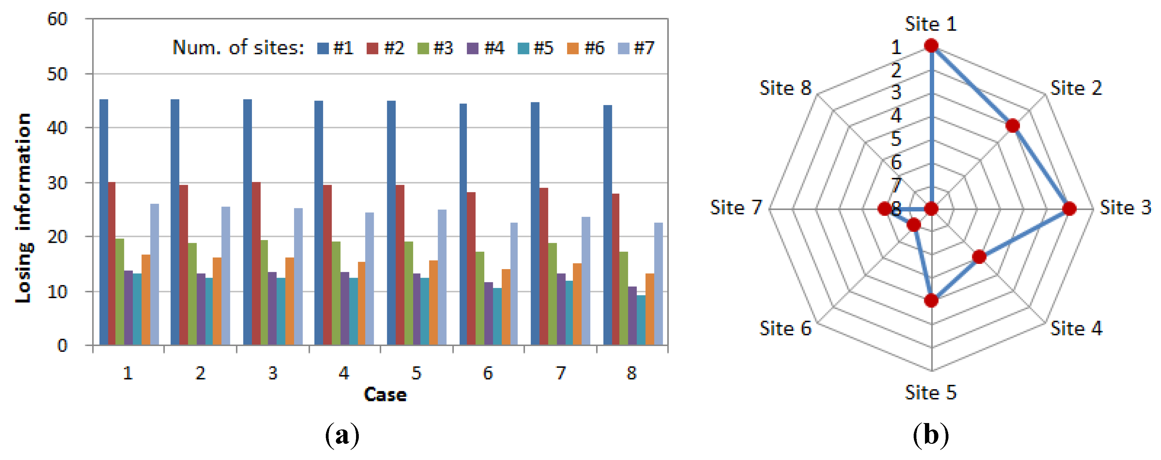
Sensitivity in each site was analyzed by calculating the losing information, which is the difference between the maximum information in each case and the maximum information from the eight sites. Here, each case means the combination of sites, with a specific site removed. For example, Case 1 estimates the maximum information using the other sites, without Site 1. Figure 4a shows the result of losing information, depending on the number of selecting sites in each case. Figure 4b shows the calculated sensitivity ranking in each site for each case. The ranking of the sites is: 1, 3, 2, 5, 7, 6 and 8.

Figure 4. Sensitivity analysis. (a) Losing information in each case; (b) Sensitivity ranking.

Figure 4. Sensitivity analysis. (a) Losing information in each case; (b) Sensitivity ranking.

3.3. Model Setup and Calibration

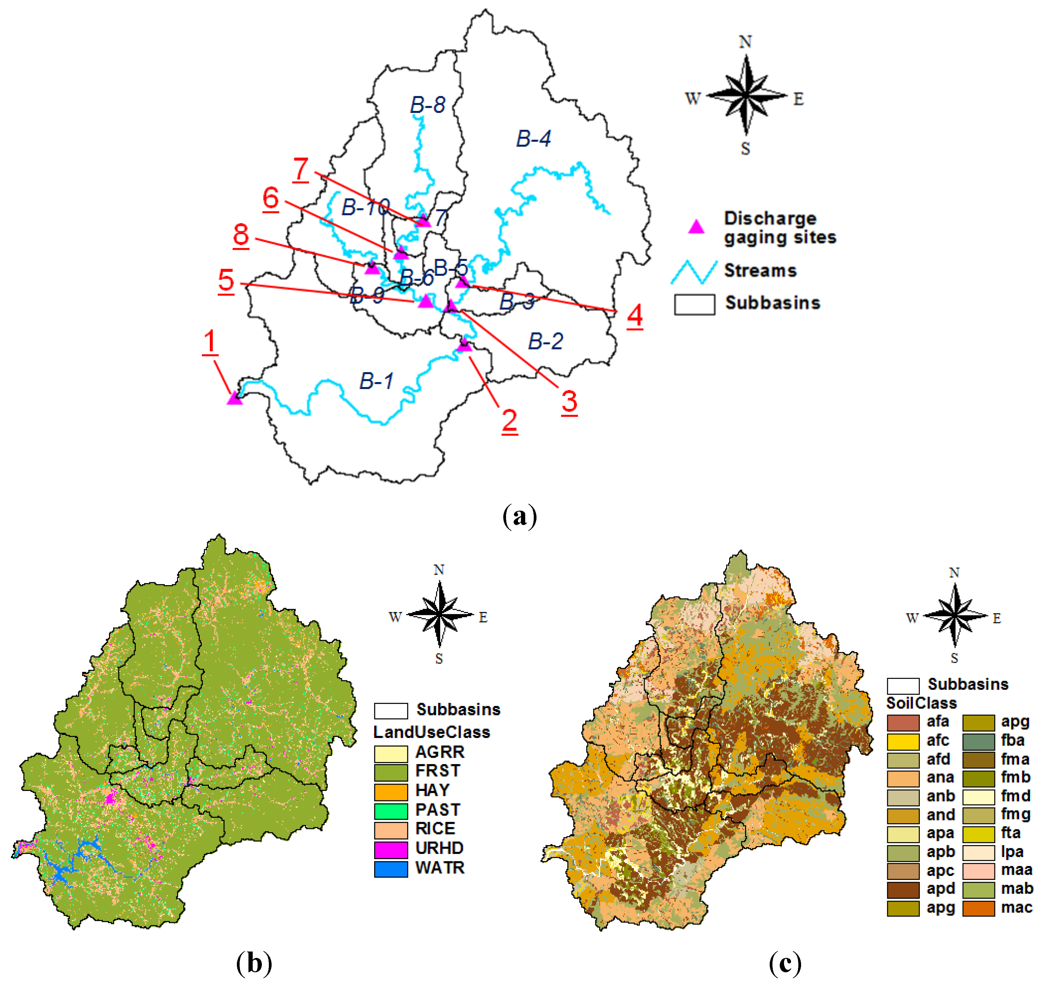
A rainfall-runoff model was built for the study basin using SWAT. Maps of 1:25,000 scale were collected to generate a 50 × 50 m² Digital Elevation Model (DEM) and a stream network. In addition, a land cover map (Figure 5b) and a soil map (Figure 5c) from the National Water Resources Management Information System (WAMIS; http://www.wamis.go.kr/) were used. The basin was classified into eight different land-use conditions, among which forests (82.2%) and rice paddies (10.3%) accounted for 92.5% of the land use. The soil map, which included classifications of 141 total types of soil, showed that apb (17.8%) and ana (15.5%) were the most prevalent soil types in the area. To build the model used for the study, GIS data were prepared to generate hydrological response units, based on the above data. Terrain analyses were conducted to delineate the channel network using the DEM of the Chungju Dam basin. The basin was divided into ten sub-basins, as shown in Figure 5a. The extract geomorphological characteristics in each sub-basin are shown in Table 4.

Figure 5. GIS data as SWAT input. (a) Stream network and sub-basins map; (b) Land use map; (c) Soil type map.

Figure 5. GIS data as SWAT input. (a) Stream network and sub-basins map; (b) Land use map; (c) Soil type map.

Table 4. Geomorphological characteristics in each sub-basin.

Sub-Basin	Basin			Stream					Remark
	Area (km2)	Slope (%)	Altitude (El. m)	Upstream Area (km2)	Length (km)	Slope (%)	Min. Alt. (El. m)	Max. Alt. (El. m)
B-1	1905.1	27.2	391.0	6631.4	101.5	10.2	71.0	174.0	Site 1
B-2	553.6	35.0	487.0	4726.2	16.4	29.3	157.0	205.0	Site 2
B-3	164.6	33.7	243.0	2398.5	12.0	70.9	136.0	221.0	Site 3
B-4	2233.9	32.2	667.0	2233.9	128.9	30.2	216.0	605.0	Site 4
B-5	276.9	22.6	328.0	1774.2	26.8	17.9	193.0	241.0	Site 5
B-6	88.5	28.6	421.0	896.1	19.3	56.9	215.0	325.0	–
B-7	110.1	31.1	476.0	807.5	23.7	33.0	257.0	335.0	Site 6
B-8	697.4	28.5	636.0	697.4	52.4	47.0	291.0	537.0	Site 7
B-9	67.3	21.1	351.0	601.2	14.0	28.5	211.0	251.0	–
B-10	533.9	26.0	548.0	533.9	43.2	44.0	251.0	441.0	Site 8

Table 4. Geomorphological characteristics in each sub-basin.

Sub-Basin	Basin			Stream					Remark
	Area (km2)	Slope (%)	Altitude (El. m)	Upstream Area (km2)	Length (km)	Slope (%)	Min. Alt. (El. m)	Max. Alt. (El. m)
B-1	1905.1	27.2	391.0	6631.4	101.5	10.2	71.0	174.0	Site 1
B-2	553.6	35.0	487.0	4726.2	16.4	29.3	157.0	205.0	Site 2
B-3	164.6	33.7	243.0	2398.5	12.0	70.9	136.0	221.0	Site 3
B-4	2233.9	32.2	667.0	2233.9	128.9	30.2	216.0	605.0	Site 4
B-5	276.9	22.6	328.0	1774.2	26.8	17.9	193.0	241.0	Site 5
B-6	88.5	28.6	421.0	896.1	19.3	56.9	215.0	325.0	–
B-7	110.1	31.1	476.0	807.5	23.7	33.0	257.0	335.0	Site 6
B-8	697.4	28.5	636.0	697.4	52.4	47.0	291.0	537.0	Site 7
B-9	67.3	21.1	351.0	601.2	14.0	28.5	211.0	251.0	–
B-10	533.9	26.0	548.0	533.9	43.2	44.0	251.0	441.0	Site 8

In this study, surface runoff was estimated using the Soil Conservation Service Curve Number, which has an advantage to predict direct runoff or infiltration from excess rainfall using daily precipitation and GIS data like soil type and land-use maps in an ungagged area. Any water that does not become surface runoff enters the soil column, where it is removed through evapotranspiration or through deep percolation into the deep aquifer, or the runoff may move laterally in the soil column as a streamflow contribution. Groundwater contribution to streamflow is generated from both shallow and deep aquifers, and is based on groundwater balance. There are three methods for estimating evapotranspiration like Priestley-Taylor, Penman-Monteith, and Hargreaves in SWAT. The Penman-Monteith method [56] was used to estimate evapotranspiration using weather variables, such as mean temperature, wind speed, relative humidity, and solar radiation.

SWAT contains several parameters that are used to describe the spatially distributed movement of water through the watershed system. Some of these parameters, such as the Curve Number (CN), cannot be directly measured and must be estimated through calibration. SWAT is a distributed hydrological model and consequently there are potentially many (thousands) parameters. As it is impossible to calibrate all of them, a reduction of the number of parameters to estimate is inevitable. In this study, seven parameters that govern the surface water response and the subsurface water response of SWAT were used in the calibration. Table 5 shows a general description of the seven parameters [57]. The default parameters were determined by the methods introduced by Neitsch, et al. [58]. A more detailed presentation for primary parameters and sensitivity tests is referred in many studies [57,58,59,60,61].

There are several automatic calibration algorithms. Zhang, et al. [32] compared the efficacy of five global optimization algorithms, such as shuffled complex evolution method developed at The University of Arizona (SCE-UA), Genetic Algorithms (GA), Particle Swarm Optimization (PSO), Artificial Immune Systems (AIS), and Differential Evaluation (DE), for calibrating SWAT and found that GA is a promising single-objective optimization method. This study used GA to estimate the optimized parameters of SWAT. In GA, a roulette wheel algorithm is used to select chromosomes for the crossover and the mutation operations [62]. A two-point crossover method with a probability of 0.8 was selected for making the search shorter and more robust, and a mutation with a probability of 0.01 was selected. The RMSE fitness function (Fs) [25] was used in this study. This performance index was defined to minimize the RMSE, as shown in Equation (13):

$$\text{Fs}=\text{min}\left(\text{RMSE}\right)=\text{min}\left(\sqrt{\frac{1}{n}{{\displaystyle \sum }}^{\text{}}(y_i-\widehat{y_l})}\right)$$

(13)

where $y_i$ is simulated daily discharge, $\widehat{y_{\text{l}}}$ is observed daily discharge at the calibration site, and n is the number of days with observations.

Table 5. Parameters for the calibration of SWAT.

Num.	Parameter	Description	Range
Parameters governing surface water response
1	CN2	Curve number 2	35–98
2	ESCO	Soil evaporation compensation factor	0–1
3	SOL_AWC	Available soil water capacity	0–1
Parameters governing subsurface water response
4	GWQMN	Threshold depth of water in the shallow aquifer for return flow to occur (mm)	0–5000
5	REVAPMN	Threshold depth of water in the shallow aquifer for reevaporation to occur (mm)	0–500
6	GW_REVAP	Groundwater reevaporation coefficient	0.02–0.2
7	ALPHA_BF	Base flow recession constant	0–1

Table 5. Parameters for the calibration of SWAT.

Num.	Parameter	Description	Range
Parameters governing surface water response
1	CN2	Curve number 2	35–98
2	ESCO	Soil evaporation compensation factor	0–1
3	SOL_AWC	Available soil water capacity	0–1
Parameters governing subsurface water response
4	GWQMN	Threshold depth of water in the shallow aquifer for return flow to occur (mm)	0–5000
5	REVAPMN	Threshold depth of water in the shallow aquifer for reevaporation to occur (mm)	0–500
6	GW_REVAP	Groundwater reevaporation coefficient	0.02–0.2
7	ALPHA_BF	Base flow recession constant	0–1

The size of the initial population was set to 50, and the number of generations was set to 1000. The sites were selected according to the entropy method. The algorithm was configured so that optimization was implemented sequentially, starting with the discharge-gauging site that was the furthest upstream. For example, if calibration is conducted for the case where there are three observation station sites (Sites 1, 3, and 7), then Site 7, which is the furthest upstream, would be the first to be calibrated, followed by Site 3 and Site 1.

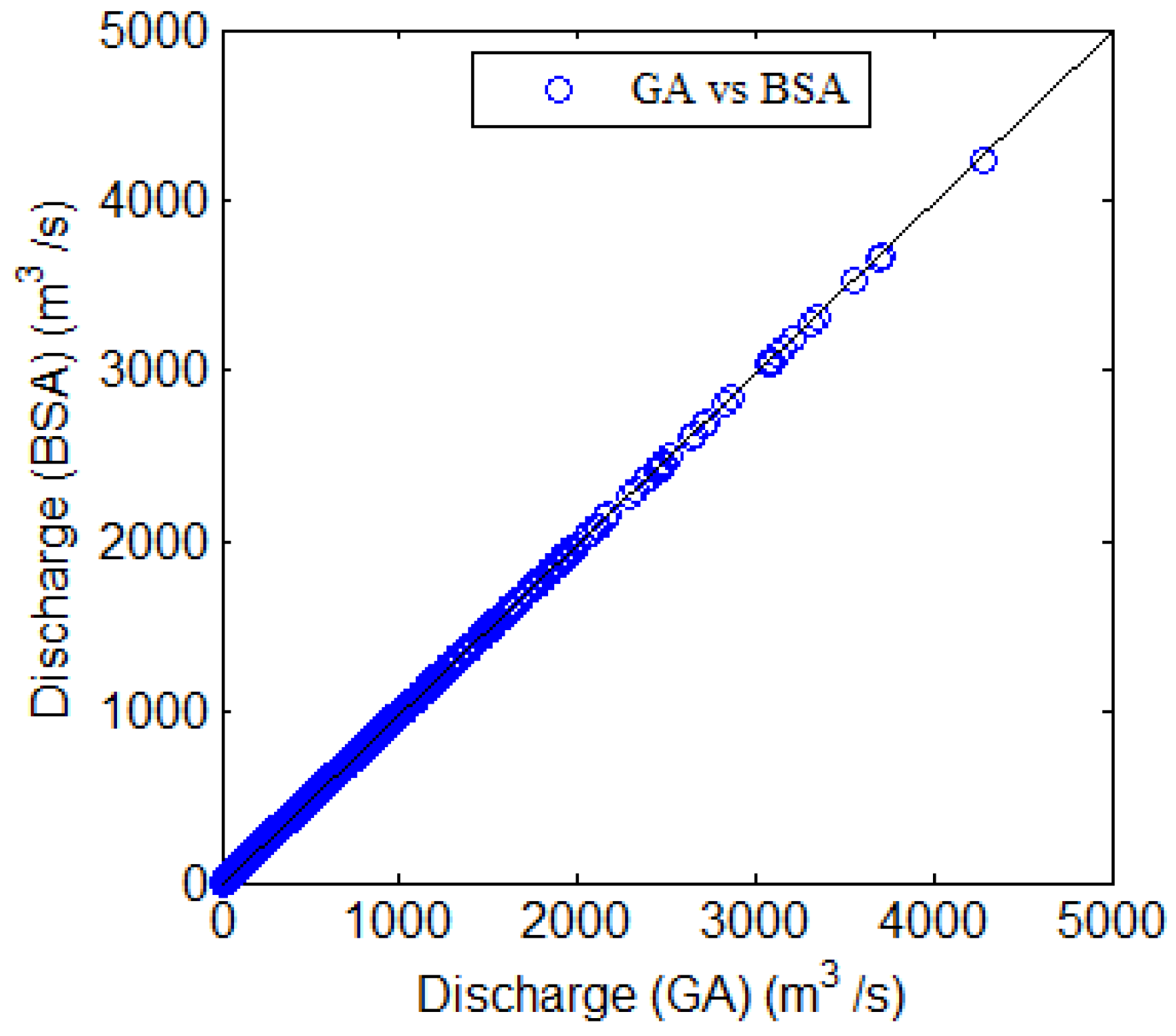
The GA for the parameter optimization of the SWAT in this study was tested by comparing it to a simple Brute-force Search Algorithm (BSA) for checking the applicability of GA. The calibration was only performed at the outlet site of the whole basin. The optimized parameters in each algorithm are shown in Table 6. The parameters were remarkably similar and the RMSE between the results (from Figure 6) using these methods was about 0.07 m³/s. This shows both the applicability of the GA and its usefulness in solving the problem of complex combinations in this study.

Table 6. Optimized parameters by GA and BSA.

Parameter	GA	BSA
CN2	48	48
ESCO	0.73	0.8
SOL_AWC	0.32	0.3
GWQMN	1694	1600
REVAPMN	132	150
GW_REVAP	0.08	0.1
ALPHA_BF	0.6	0.5

Table 6. Optimized parameters by GA and BSA.

Parameter	GA	BSA
CN2	48	48
ESCO	0.73	0.8
SOL_AWC	0.32	0.3
GWQMN	1694	1600
REVAPMN	132	150
GW_REVAP	0.08	0.1
ALPHA_BF	0.6	0.5

Figure 6. Discharge comparison of GA vs. BSA.

Figure 6. Discharge comparison of GA vs. BSA.

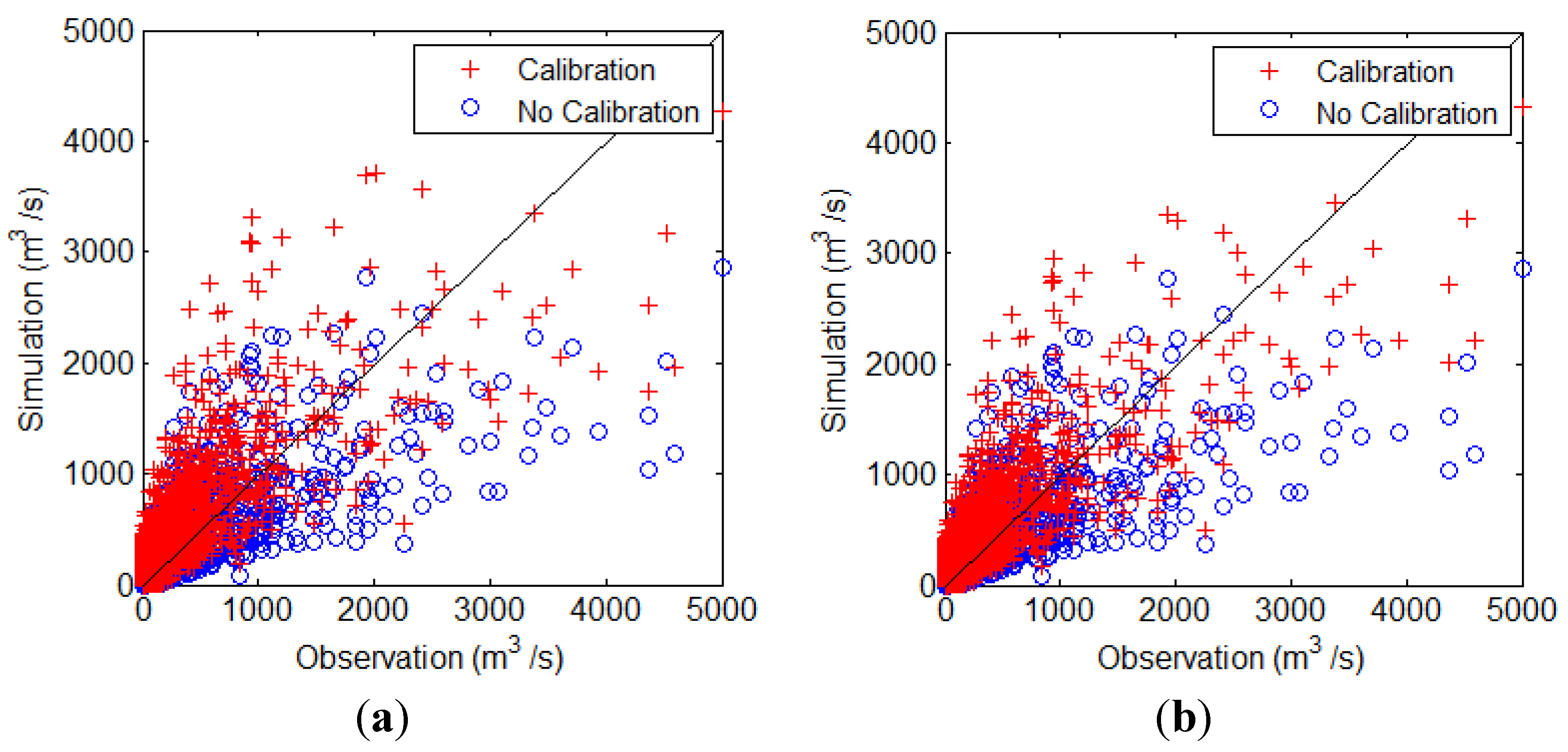
Using the above method, calibration was conducted at the respective sites. Table 3 was referenced for all of the cases where the number of sites selected was one to eight. After the respective cases were calibrated, the relation between observed daily discharge and simulated daily discharge at the eight discharge-gauging sites in the study basin was illustrated, as shown in Figure 7. Figure 7a shows the case where calibration was conducted at only one site (Case 1), whereas Figure 7b shows the case where calibration was performed at five different sites (Case 5). These cases were compared to the case where no calibration was conducted (no calibration; blue circle). Case 5 is included in the comparison because the maximum amount of information was indicated when five sites (Sites 1, 2, 3, 5, and 6) were selected in the study basin (see Table 3). It was determined that the simulated discharge in the case where no calibration was conducted had an underestimation issue (blue circles), and Case 5 (five sites selected) produced a better result than Case 1 (one site selected).

Figure 7. Scatter plot for the relation between observation and simulation. (a) Calibration at one site (Case 1); (b) Calibration at five sites (Case 5).

Figure 7. Scatter plot for the relation between observation and simulation. (a) Calibration at one site (Case 1); (b) Calibration at five sites (Case 5).

3.4. Calibration Results and Discussion

The calibration results, based on the respective results of Table 3 (from #1 to #8), were mutually compared. Three evaluation functions were applied for the observed and simulated discharges, coefficient of correlation (CC), RMSE, and Nash-Sutcliffe efficiency (NSE) [63]. The results of the case evaluations (with the selection of one to eight sites) using the evaluation functions are shown in Table 7 and Figure 8. The evaluation was conducted for all of the sites and for the outlet. First, the calibration results were applied to all of the sites for comparison. Even if only one site had been selected for calibration, it would have been compared with the respective observation discharge of eight sites after the simulated discharge of eight sites was extracted. 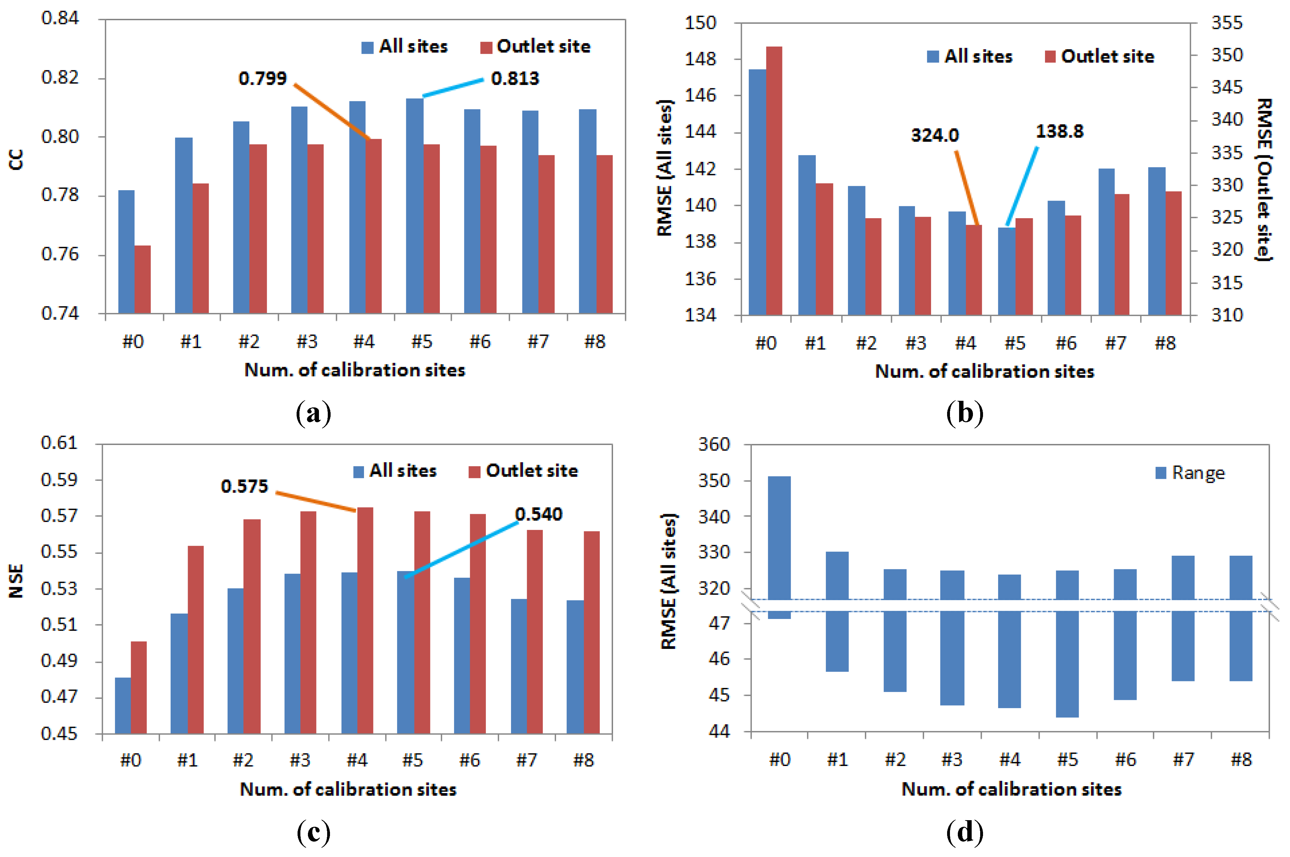Next, the outlet from the most important site (as determined in Table 3) was applied. The applicability of the SWAT model was outstanding in the study basin as the CC, RMSE, and NSE were 0.782, 147.4, and 0.482, respectively, even in the case where no calibration was conducted (#0); however, it was confirmed that the results were improved slightly when the model was calibrated. In particular, the result of the case with more sites selected was even better than the result of the case with only one site selected. Nevertheless, the calibration result did not improve any further when the number of sites selected exceeded a certain number. This characteristic is easily confirmed through Figure 8 and Case 5, where all of the sites were evaluated (five sites selected: CC, 0.813; RMSE, 138.8; NSE, 0.540), and Case 4, where the basin outlet point was evaluated (four sites selected: CC, 0.799; RMSE, 324.0; NSE, 0.575) and the best calibration result was produced. If the case evaluating all of the discharge-gauging sites in the basin is deemed to be more representative than the case evaluating only the outlet point of the basin, then Case 5, where five sites (Sites 1, 2, 3, 5, and 6) were selected for calibration, produces the best result.

Table 7. Calibration results at all sites and the outlet site.

Site Number	All Sites			Outlet Site
	CC	RMSE (m3/s)	NSE	CC	RMSE (m3/s)	NSE
#0 (Non-C.)	0.782	147.4	0.482	0.763	351.3	0.501
#1	0.800	142.8	0.516	0.784	330.4	0.554
#2	0.805	141.1	0.530	0.798	325.2	0.568
#3	0.810	140.0	0.538	0.798	325.1	0.573
#4	0.812	139.7	0.539	0.799	324.0	0.575
#5	0.813	138.8	0.540	0.798	325.1	0.573
#6	0.809	140.3	0.536	0.797	325.5	0.572
#7	0.809	142.1	0.524	0.794	329.0	0.562
#8	0.809	142.1	0.524	0.794	329.2	0.562

Table 7. Calibration results at all sites and the outlet site.

Site Number	All Sites			Outlet Site
	CC	RMSE (m3/s)	NSE	CC	RMSE (m3/s)	NSE
#0 (Non-C.)	0.782	147.4	0.482	0.763	351.3	0.501
#1	0.800	142.8	0.516	0.784	330.4	0.554
#2	0.805	141.1	0.530	0.798	325.2	0.568
#3	0.810	140.0	0.538	0.798	325.1	0.573
#4	0.812	139.7	0.539	0.799	324.0	0.575
#5	0.813	138.8	0.540	0.798	325.1	0.573
#6	0.809	140.3	0.536	0.797	325.5	0.572
#7	0.809	142.1	0.524	0.794	329.0	0.562
#8	0.809	142.1	0.524	0.794	329.2	0.562

The total information will increase if more sites are used. For example, the maximum information was about 66 when eight sites were used in this study (see Table 3). However, the maximum information was about 56.6 when seven sites were used in Case 8 (shown in Figure 9). Here, Case 8 means that Site 8 was removed from the eight sites and the maximum information is calculated using the other seven sites. There is a small difference between using seven sites among seven sites and using seven sites among eight sites. The maximum information was 59.1 when seven sites were selected among eight sites. However, the maximum information was shown when five sites (1, 2, 3, 5, and 6 sites) were selected among the eight sites. As a result, if in the future more observation sites are available, it will still be possible to get more information. However, the maximum information is not shown when all observation sites are used.

Figure 8. Calibration results using evaluation functions. (a) Coefficient of correlation; (b) RMSE; (c) NSE; (d) RMSE range in case of all sites.

Figure 8. Calibration results using evaluation functions. (a) Coefficient of correlation; (b) RMSE; (c) NSE; (d) RMSE range in case of all sites.

Figure 9. Maximum information using seven total sites.

Figure 9. Maximum information using seven total sites.

The entropy method may identify the number of calibration sites after which the marginal increase in model efficiency to represent the observed runoff no longer significantly increases. Choi, et al. [31] stated that additional calibration sites can benefit model performance. However, the results of this study showed that model performance instead decreased if more four of five sites were selected (Table 7). There may be two reasons for this. First, the exclusion of one of the sites worsened the simulation result of the other sites. The sites that caused this response could be Site 4 and Site 8 because model performance with those sites is decreased. However, there is a limit to understanding the result of the model performance using only one problem in each site. This does not clearly explain the results in terms of Site 7. In fact, the model performance for Site 7 is positive in Case 3 and Case 4, and negative in Case 8 (as seen Table 3 and Table 7). Here, error compensation is a very important point for multi-site calibration. In a case where many sites are considered for calibration, error compensation has an effect on model performance. In this study, error compensation can be prevented if all of the sites are used for calibration, and therefore decrease model performance. Model performance will increase due solely to the error compensation if fewer than the maximum number of sites is used for calibration. Therefore, the entropy method should not be preferred over an approach where all available sites are used for calibration, if time allows for it. The entropy method is useful in cases where computational requirements do not allow the use of all sites for calibration. In other words, the entropy method is only useful in reducing the time and effort of model calibration, but not in increasing model performance.

The growing importance of water resource management, along with the development of observation techniques, has recently resulted in the installation of significantly more water level observation stations in basins. Currently, there are 21 water level observation stations in the study basin, and it is expected that the observed discharge information will be continuously accumulated. Obviously, observation data obtained from more sites will be a great advantage to hydrological modeling. However, assuming that all 21 sites in the study basin can be utilized, the number of cases of the selection of sites for calibration is 2,097,151 ($\sum _{\text{n}=1}^{21}$₂₁C_n= 2,097,151). While this assumption does not consider the importance of the sites, the number of cases for the hydrological model calibration must still be high. If the brute-force search method is considered to select calibration sites in this area, we would waste too much time and effort. Sometimes, a modeling result does not improve any further, although we try to get a good result in model calibration. This study confirmed that the selection of more calibration sites did not lead to improved calibration results from the model. Therefore, the entropy method attempted in this study is expected to provide an excellent guideline to conduct the calibration of the hydrological model. In addition, the application of the theory will further increase when selecting a certain number of sites, depending on the purpose of the application of the model, because the theory also provides information as to which sites need to be selected.

4. Conclusions

The purpose of this study was to review the applicability of the entropy method in selecting the calibration sites for hydrological modeling. The entropy method was applied to the discharge data of eight different sites in the Chungju Dam Basin in Korea. Then, the selected sites were combined, case-by-case, so that the combination of sites can yield the maximum amount of information. In addition, the SWAT model was established for the study basin, and the model was calibrated by estimating the optimal parameters using a genetic algorithm at the discharge-gauging sites selected through the entropy method. As a result, we learned that the model calibration using the selected sites and the combined sites having maximum information based on the entropy method gave us excellent outcomes. Therefore, we confirmed the applicability of the entropy theory in the selection of calibration sites for hydrological modeling. In addition, the entropy method is only useful in reducing the time and effort spent on model calibration, but not in increasing model performance. The method needs to apply and evaluate its applicability through various hydrological models in the future.

In particular, selecting more sites does not always lead to a better model performance. The decrease in model performance when selecting more than the optimal number of sites indicated by the entropy method can be associated to error compensation. However, applying the entropy method can significantly reduce time and effort required for model calibration, and can therefore be a valuable tool if the computational requirements for parameter optimization against all available data exceed available resources. As more discharge-gauging stations are expected to be installed all over the world, the entropy method, which provides information on the preferential types of observation stations to consider for the calibration of the hydrological model, will have significantly more use in the future.

References

1. Moriasi, D.N.; Wilson, B.N.; Douglas-Mankin, K.R.; Arnold, J.G.; Gowda, P.H. Hydrologic and water quality models: Use, calibration, and validation. Trans. ASABE 2012, 55, 1241–1247. [Google Scholar] [CrossRef]
2. Beven, K. Changing ideas in hydrology—The case of physically based models. J. Hydrol. 1989, 105, 157–172. [Google Scholar] [CrossRef]
3. Duan, Q.Y.; Sorooshian, S.; Gupta, V. Effective and efficient global optimization for conceptual rainfall-runoff models. Water Resour. Res. 1992, 28, 1015–1031. [Google Scholar] [CrossRef]
4. Beven, K.J.; Binley, A.M. The future of distributed models: Model calibration and uncertainty prediction. Hydrol. Process. 1992, 6, 279–298. [Google Scholar] [CrossRef]
5. Beven, K. Prophecy, reality, and uncertainty in distributed hydrological modeling. Adv. Water Resour. 1993, 16, 41–51. [Google Scholar] [CrossRef]
6. Oudin, L.; Perrin, C.; Mathevet, T.; Andréassian, V.; Michel, C. Impact of biased and randomly corrupted inputs on the efficiency and the parameters of watershed models. J. Hydrol. 2006, 320, 62–83. [Google Scholar] [CrossRef]
7. Tang, Y.; Reed, P.; van Werkhoven, K.; Wagener, T. Advancing the identification and evaluation of distributed rainfall-runoff models using global sensitivity analysis. Water Resour. Res. 2007, 43. [Google Scholar] [CrossRef]
8. Engel, B.; Storm, D.; White, M.; Arnold, J.; Arabi, M. A hydrologic/water quality model application protocol. J. Am. Water Resour. Assoc. 2007, 43, 1223–1236. [Google Scholar] [CrossRef]
9. Moriasi, D.N.; Arnold, J.G.; van Liew, M.W.; Bingner, R.L.; Harmel, R.D.; Veith, T.L. Model evaluation guidelines for systematic quantification of accuracy in watershed simulations. Trans. ASABE 2007, 50, 885–900. [Google Scholar] [CrossRef]
10. Harmel, R.D.; Smith, P.K.; Migliaccio, K.L. Modifying goodness-of-fit indicators to incorporate both measurement and model uncertainty in model calibration and validation. Trans. ASABE 2010, 53, 55–63. [Google Scholar] [CrossRef]
11. Pushpalatha, R.; Perrin, C.; le Moine, N.; Mathevet, T.; Andréassian, V. A downward structural sensitivity analysis of hydrological models to improve low-flow simulation. J. Hydrol. 2011, 411, 66–76. [Google Scholar] [CrossRef]
12. Beven, K.; O’Connell, P.E. On the Role of a Physically Based Distributed Modeling in Hydrology; Institute of Hydrology: Wallingford, UK, 1982. [Google Scholar]
13. Abbott, M.B.; Bathurst, J.C.; Cunge, J.A.; O’Connell, P.E.; Rasmussen, J. An introduction to the European hydrological system—Systeme hydrologique Europeen, “SHE,” 1: History and philosophy of a physically based, distributed modelling system. J. Hydrol. 1986, 87, 45–59. [Google Scholar] [CrossRef]
14. Refsgaard, J.C.; Storm, B. Construction, Calibration and Validation of Hydrological Models. In Distributed Hydrological Modeling; Kluwer Academic: Dordrecht, The Netherlands, 1996; pp. 41–54. [Google Scholar]
15. Lee, H.; McIntyre, N.; Wheater, H.; Young, A. Selection of conceptual models for regionalization of the rainfall-runoff relationship. J. Hydrol. 2005, 312, 125–147. [Google Scholar] [CrossRef]
16. Sahoo, G.B.; Ray, C.; de Carlo, E.H. Calibration and validation of a physically distributed hydrological model, MIKE SHE, to predict streamflow at high frequency in a flashy mountainous Hawaii stream. J. Hydrol. 2006, 327, 94–109. [Google Scholar] [CrossRef]
17. Hu, W.; Shao, M.; Wang, Q.; She, D. Effects of measurement method, scale, and landscape features on variability of saturated hydraulic conductivity. J. Hydrol. Eng. 2013, 18, 378–386. [Google Scholar] [CrossRef]
18. Gholami, V.; Chau, K.W.; Fadaee, F.; Torkaman, J.; Ghaffari, A. Modeling of groundwater level fluctuations using dendrochronology in alluvial aquifers. J. Hydrol. 2015, 529, 1060–1069. [Google Scholar] [CrossRef]
19. Taormina, R.; Chau, K.W. ANN-based interval forecasting of streamflow discharges using the LUBE method and MOFIPS. Eng. Appl. Artif. Intell. 2015, 45, 429–440. [Google Scholar] [CrossRef]
20. Wu, C.L.; Chau, K.W.; Li, Y.S. Methods to improve neural network performance in daily flows prediction. J. Hydrol. 2009, 372, 80–93. [Google Scholar] [CrossRef]
21. Wang, W.C.; Chau, K.W.; Xu, D.M.; Chen, X.Y. Improving forecasting accuracy of annual runoff time series using ARIMA based on EEMD decomposition. Water Resour. Manag. 2015, 29, 2655–2675. [Google Scholar] [CrossRef]
22. Chen, X.Y.; Chau, K.W. A comparative study of population-based optimization algorithms for downstream river flow forecasting by a hybrid neural network model. Eng. Appl. Artif. Intell. 2015, 46, 258–268. [Google Scholar] [CrossRef]
23. Chau, K.W.; Wu, C.L. A hybrid model coupled with singular spectrum analysis for daily rainfall prediction. J. Hydroinform. 2010, 12, 458–473. [Google Scholar] [CrossRef]
24. Park, M.K.; Kim, D.G.; Kwak, J.W.; Kim, H.S. Evaluation of parameter characteristics of the storage function model. J. Hydrol. Eng. 2014, 19, 308–318. [Google Scholar] [CrossRef]
25. Hogue, T.S.; Sorooshian, S.; Gupta, H.V.; Holz, A.; Braatz, D. A multi-step automatic calibration scheme (MACS) for river forecasting models. J. Hydrometeorol. 2000, 1, 524–542. [Google Scholar] [CrossRef]
26. Nelder, J.A.; Mead, R. A simplex method for function minimization. Comput. J. 1965, 7, 308–313. [Google Scholar] [CrossRef]
27. Wang, Q.J. The genetic algorithm and its application to calibrating conceptual rainfall-runoff models. Water Resour. Res. 1991, 27, 2467–2471. [Google Scholar] [CrossRef]
28. Ajami, N.K.; Gupta, H.; Wagener, T.; Sorooshian, S. Calibration of a semidistributed hydrologic model for streamflow estimation along a river system. J. Hydrol. 2004, 298, 112–135. [Google Scholar] [CrossRef]
29. Merz, R; Blöschl, G. Regionalisation of catchment model parameters. J. Hydrol. 2004, 287, 95–123. [Google Scholar] [CrossRef]
30. Young, A. Streamflow simulation within UK ungauged catchments using a daily rainfall-runoff model. J. Hydrol. 2006, 320, 155–172. [Google Scholar] [CrossRef]
31. Choi, Y.S.; Choi, C.K.; Kim, H.S.; Kim, K.T.; Kim, S. Multi-site calibration using a grid-based event rainfall-runoff model: A case study of the upstream areas of the Nakdong River basin in Korea. Hydrol. Process. 2015, 29, 2089–2099. [Google Scholar] [CrossRef]
32. Zhang, X.; Srinivasan, R.; van Liew, M. Multi-site calibration of the SWAT model for hydrologic modeling. Trans. ASABE 2008, 51, 2039–2049. [Google Scholar] [CrossRef]
33. Shannon, C.E.; Weaver, W. The Mathematical Theory of Communication; University of Illinois Press: Urbana, IL, USA, 1949. [Google Scholar]
34. Yang, Y.; Burn, D.H. An entropy approach to data collection network design. J. Hydrol. 1994, 157, 307–324. [Google Scholar] [CrossRef]
35. Amorocho, J.; Espildora, B. Entropy in the assessment of uncertainty in hydrologic systems and models. Water Resour. Res. 1973, 9, 1511–1522. [Google Scholar] [CrossRef]
36. Chapman, T.G. Entropy as a measure of hydrologic data uncertainty and model performance. J. Hydrol. 1986, 85, 111–126. [Google Scholar] [CrossRef]
37. Husain, T. Hydrologic uncertainty measure and network design. Water Resour. Bull. 1989, 25, 527–534. [Google Scholar] [CrossRef]
38. Al-Zahrani, M.; Husain, T. An algorithm for designing a precipitation network in the southwestern region of Saudi Arabia. J. Hydrol. 1998, 205, 205–216. [Google Scholar] [CrossRef]
39. Holland, J.H. Adaptation in Natural and Artificial Systems; University of Michigan Press: Ann Arbor, MI, USA, 1975. [Google Scholar]
40. Ragab, R.; Austin, B.; Moidinis, D. The HYDROMED model and its application to semi-arid Mediterranean catchments with hill reservoirs 1: The rainfall-runoff model using a genetic algorithm for optimisation. Hydrol. Earth Syst. Sci. 2001, 5, 543–553. [Google Scholar]
41. Bhattacharjya, R.K. Optimal design of unit hydrographs using probability distribution and genetic algorithms. SADHANA Acad. Proc. Eng. Sci. 2004, 29, 499–508. [Google Scholar] [CrossRef]
42. Chang, C.L.; Lo, S.L.; Yu, S.L. The parameter optimization in the inverse distance method by genetic algorithm for estimating precipitation. Environ. Monit. Assess. 2006, 117, 145–155. [Google Scholar] [CrossRef] [PubMed]
43. Refsgaard, J.C.; Storm, B. MIKE SHE. In Computer Models of Watershed Hydrology; Singh, V.P., Ed.; Water Resources Publications: Highland Ranch, CO, USA, 1995; pp. 809–846. [Google Scholar]
44. Leavesley, G.H.; Stannard, L.G. The Precipitation Runoff Modeling System—PRMS. In Computer Models of Watershed Hydrology; Singh, V.P., Ed.; Water Resources Publications: Highland Ranch, CO, USA, 1995; pp. 281–310. [Google Scholar]
45. Kite, G.W. The SLURP Model. In Computer Models of Watershed Hydrology; Singh, V.P., Ed.; Water Resources Publications: Highland Ranch, CO, USA, 1995; pp. 521–562. [Google Scholar]
46. Arnold, J.G.; Srinivasan, R.; Muttiah, R.S.; Williams, J.R. Large area hydrologic modeling and assessment: Part I. model development. J. Am. Water Resour. Assoc. 1998, 34, 73–89. [Google Scholar] [CrossRef]
47. Kim, N.W.; Chung, I.M.; Kim, C.; Lee, J.; Lee, J.E. Development and applications of SWAT-K (Korea). In Soil and Water Assessment Tool (SWAT) Global Applications; World Association of Soil and Water Conservation: Bangkok, Thailand, 2009. [Google Scholar]
48. Jaynes, E.K. Information theory and statistical mechanics. Phys. Rev. 1957, 106, 620–630. [Google Scholar] [CrossRef]
49. Molgedey, L.; Ebeling, W. Local order, entropy and predictability of financial time series. Eur. Phys. J. B 2000, 15, 733–737. [Google Scholar] [CrossRef]
50. Ulaniwicz, R.E. Information theory in ecology. Comput. Chem. 2001, 25, 393–399. [Google Scholar] [CrossRef]
51. Moramarco, T.; Saltalippi, C.; Singh, V.P. Estimation of mean velocity in natural channels based on Chiu’s velocity distribution equation. J. Hydrol. Eng. 2004, 9, 42–50. [Google Scholar] [CrossRef]
52. Mogheir, Y.; de Lima, J.L.M.P.; Singh, V.P. Characterizing the spatial variability of groundwater quality using the entropy theory: І. synthetic data. Hydrol. Process. 2004, 18, 2165–2178. [Google Scholar] [CrossRef]
53. Singh, V.P. The use of entropy in hydrology and water resources. Hydrol. Process. 1997, 11, 587–626. [Google Scholar] [CrossRef]
54. Singh, V.P. The entropy theory as a tool for modeling and decision making in environmental and water resources. Water SA 2000, 26, 1–12. [Google Scholar]
55. Yoo, C.; Jung, K.; Lee, J. Evaluation of rain gauge network using entropy theory: Comparison of mixed and continuous distribution function applications. J. Hydrol. Eng. 2008, 13, 226–235. [Google Scholar] [CrossRef]
56. Monteith, J.L. Evaporation and the environment. In the state and movement of water in living organisms. In 19th Symposia of the Society for Experimental Biology; Cambridge University Press: London, UK, 1965; pp. 205–234. [Google Scholar]
57. Van Liew, M.W.; Veith, T.L.; Bosch, D.D.; Arnold, J.G. Suitability of SWAT for the conservation effects assessment project: A comparison on USDA-ARS watersheds. J. Hydrol. Eng. 2007, 12, 173–189. [Google Scholar] [CrossRef]
58. Neitsch, S.L.; Arnold, A.G.; Kiniry, J.R.; Srinivasan, J.R.; Williams, J.R. Soil and Water Assessment Tool User’s Manual; Texas Water Resources Institute: College Station, TX, USA, 2005. [Google Scholar]
59. Van Griensven, A.; Meixner, T.; Grunwald, S.; Bishop, T.; Diluzio, M.; Srinivasan, R. A global sensitivity analysis tool for the parameters of multi-variable catchment models. J. Hydrol. 2006, 324, 10–23. [Google Scholar] [CrossRef]
60. White, L.K.; Chaubey, I. Sensitivity analysis, calibration, and validations for a multisite and multivariable SWAT model. J. Am. Water Resour. Assoc. 2005, 41, 1077–1089. [Google Scholar] [CrossRef]
61. Malagò, A.; Pagliero, L.; Bouraoui, F.; Franchini, M. Comparing calibrated parameter sets of the SWAT model for the Scandinavian and Iberian peninsulas. Hydrol. Sci. J. 2015, 60, 949–967. [Google Scholar] [CrossRef]
62. Reca, J.; Martinez, J. Genetic algorithms for the design of looped irrigation water distribution networks. Water Resour. Res. 2006, 42. [Google Scholar] [CrossRef]
63. Nash, J.E.; Sutcliffe, J.V. River flow forecasting through conceptual models Part I—A discussion of principles. J. Hydrol. 1970, 10, 283–290. [Google Scholar] [CrossRef]