An Indirect Simulation-Optimization Model for Determining Optimal TMDL Allocation under Uncertainty

Abstract

An indirect simulation-optimization model framework with enhanced computational efficiency and risk-based decision-making capability was developed to determine optimal total maximum daily load (TMDL) allocation under uncertainty. To convert the traditional direct simulation-optimization model into our indirect equivalent model framework, we proposed a two-step strategy: (1) application of interval regression equations derived by a Bayesian recursive regression tree (BRRT v2) algorithm, which approximates the original hydrodynamic and water-quality simulation models and accurately quantifies the inherent nonlinear relationship between nutrient load reductions and the credible interval of algal biomass with a given confidence interval; and (2) incorporation of the calibrated interval regression equations into an uncertain optimization framework, which is further converted to our indirect equivalent framework by the enhanced-interval linear programming (EILP) method and provides approximate-optimal solutions at various risk levels. The proposed strategy was applied to the Swift Creek Reservoir’s nutrient TMDL allocation (Chesterfield County, VA) to identify the minimum nutrient load allocations required from eight sub-watersheds to ensure compliance with user-specified chlorophyll criteria. Our results indicated that the BRRT-EILP model could identify critical sub-watersheds faster than the traditional one and requires lower reduction of nutrient loadings compared to traditional stochastic simulation and trial-and-error (TAE) approaches. This suggests that our proposed framework performs better in optimal TMDL development compared to the traditional simulation-optimization models and provides extreme and non-extreme tradeoff analysis under uncertainty for risk-based decision making.

1. Introduction

Section 303(d) of the 1972 Clean Water Act requires the development of total maximum daily load (TMDL) to restore impaired water bodies [1]. TMDL refers to the maximum loading rates of a pollutant that a water body receives to ensure compliance with water-quality standards and allocates pollutant loadings among point and nonpoint sources at different risk levels [1,2]. In most TMDL allocation analyses, load reduction scenarios are generated through trial-and-error (TAE) simulation [2], which involves repeatedly running process-oriented simulation models to derive the pollutant loadings to meet water-quality standards and allocation criteria in the water body [3,4]. However, the TAE simulation method does not necessarily generate the most cost-effective and reliable load allocations [5]. To increase the financial and technical feasibility of implementation, the U.S. Environmental Protection Agency [1] suggested that process-oriented simulation models could be directly integrated into an optimization framework to develop optimal TMDL allocations at the least cost while risk must be identified. Either traditional nonlinear optimization or modern heuristic global search algorithms can be applied in the direct simulation-optimization model (SOM) framework [6,7,8,9,10,11,12,13]; however, this direct SOM approach is rarely applied in practice, primarily due to the prohibitive computational cost and the neglect of uncertainties in both simulation modeling and the optimization process [7,14].

Most of the input parameters and model structures in both simulation and optimization procedures are uncertain, which affects the decision-making process [15]. The SOM framework under uncertainty can be grouped into four broad categories: namely stochastic optimization models, fuzzy optimization models, interval optimization models and hybrids of the above three model types [15,16,17,18,19]. However, the increasing data requirements for specifying probability density or parameter membership functions have become a big challenge for TMDL allocations [7,14]. Even when many data are available, the computational algorithms for stochastic or fuzzy optimization models, such as nonlinear programming (NP) or modern heuristic global searches, may face complex or nonlinear problems [19,20]. For example, traditional NP algorithms, including both gradient and non-gradient based ones, were limited to local optima upon solving the aforementioned SOM framework [11,21]. Although heuristic global search algorithms, including genetic algorithms, evolutionary algorithms and simulated annealing, are capable of surpassing the local optima limitations, their applications in the optimization of TMDL allocation are still restricted by their extremely high computational cost [18,22].

To mitigate the above problems, the interval linear programming (ILP) model [16], which does not require probability density or membership function, could be a potential alternative to stochastic or fuzzy optimization models. Based on Huang’s cluster analysis [16], Zhou et al. [23] proposed a modified interval linear programming (MILP) model to establish strict mathematical relationships between decision variables and uncertain constraint coefficients, which also provides sufficient conditions to obtain an absolutely feasible solution space. Zhou et al. [19] further defined a new uncertainty type, the enhanced-interval number, and developed an enhanced-interval linear programming (EILP) model, as well as a computationally-efficient solution algorithm, which provides insight into both extreme and non-extreme tradeoffs between system benefits and the different risk levels of constraint violations due to parametric uncertainties in the objective functions and constraints [15,18].

Several functional approximators have been developed for building the response function of water quality to pollutant loadings and to overcome the computation bottleneck associated with direct SOM applications. This indirect SOM framework, in place of complex process-oriented models, incorporates an approximation function into an optimization model for searching optimal TMDL allocations [7,8,24]. Generally, the framework with the approximation function needs to be sufficiently generalized to achieve optimal or approximate-optimal solutions of the original direct SOM system. This means that the regression tree model [25], the response surface [14] or the artificial neural network (ANN) [22] should truly capture the underlying functional form of the simulation model rather than just the training data used to calibrate the models. Although the ANN approach is one powerful platform for developing an approximation function, it has not yet been shown to provide explicit expressions of nonlinear stressor-response relationships and effectively quantify uncertainties in dynamic water body systems. Recently, the Bayesian recursive regression tree Version 2 (BRRT v2) model was developed for rapidly capturing the nonlinear stressor-response relationship of general aquatic systems [26], generating a series of interval linear regression equations that covered the pertinent ranges of stressors and responses reflected in the original nonlinear simulation model. Given its computational efficiency, predictive accuracy and capability of explicitly quantifying uncertainty in previous works [26], the BRRT v2 may be employed as a surrogate for a simulation model in an indirect SOM framework by replacing the process-oriented simulation model with interval linear regression equations.

The purpose of this paper is to propose an indirect SOM framework by integrating the BRRT v2 and EILP models for risk-based optimal TMDL allocation, which guarantees the approximate-optimal solutions with relatively low computational cost and to provide extreme and non-extreme tradeoff analysis for risk-based decision making. The risk-based optimal TMDL allocation aims to determine the optimal required pollutant removal rates from point and nonpoint sources to ensure compliance with water-quality standards under different risk levels. Using the real-world case study in the Swift Creek Reservoir watershed (Chesterfield County, VA), we compared the performance of the proposed BRRT-EILP model with the direct simulation-optimization model, stochastic simulation and TAE approaches in terms of computational efficiency and risk-based decision-making capability for TMDL allocation under uncertainty.

2. Materials and Methods

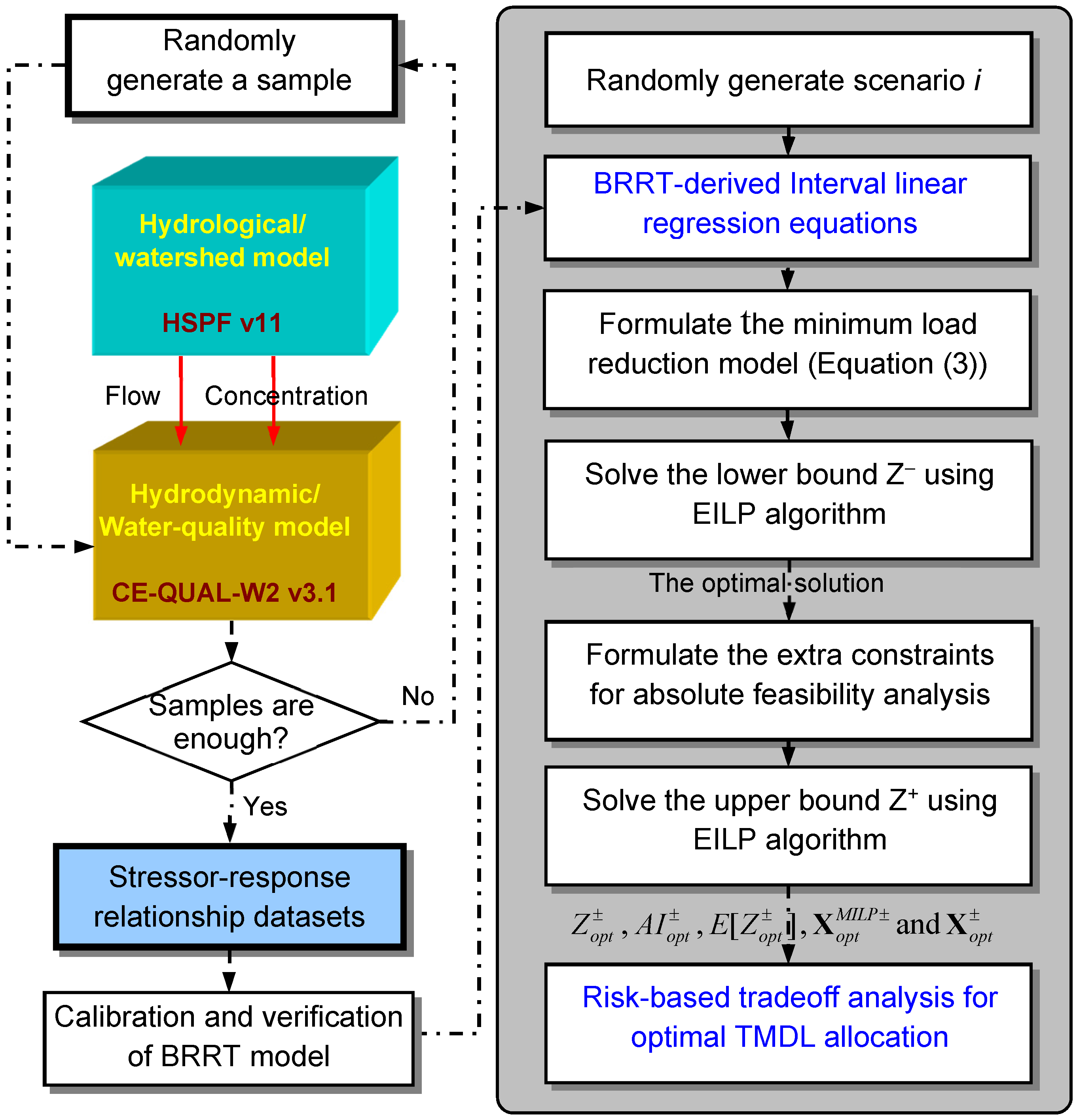
2.1. BRRT-EILP Model

The combined BRRT-EILP model consists of two critical components: (i) the simulation model for predicting nonlinear responses to pollutant removal rates among all pollution sources; and (ii) the optimization model for achieving the optimal pollutant removal rates under uncertainty [1]. A general direct SOM model framework under uncertainty was developed to minimize load reductions as follows:

$$Min{Z}^{\pm }=C^{\pm }{X}^{\pm },s.t{Y}^{\pm }\text{= }h(X^{\pm },A^{\pm })\le Y^{*\pm },X^{\pm }\ge 0$$

(1)

where $X^{\pm }$ represents the pollutant removal rates, $Z^{\pm }$ is the total load reductions, $Y^{i\pm }$ is the simulated concentration of pollutants, $Y^{*\pm }$ is the user-specified water-quality criteria, $A^{\pm }$ is the parameters for process-oriented models (i.e., $Y^{\pm }\text{= }h(X^{\pm },A^{\pm })$) and $B^{\pm }$ and $C^{\pm }$ are the coefficients of the constraints or objective function. All parameters above are also defined as interval numbers due to the systematic uncertainty propagated from sampling collection, water quality model (i.e., structure and parameters), and coefficients in the optimization model [27,28]. Based on the experience of TMDL in the United States [1], the objective function $Z^{\pm }$ is usually defined as an acceptable measure of economic efficiency, reliability and equity. When detailed cost information is not available, minimizing load reduction could be used as an alternative to maximize the economic efficiency, since we would at least expect increased system costs for a given pollution source following increased load reduction [2]. The objective function used in this study was eventually used to determine the required minimum total load reductions; the system constraints in Equation (1) were to bring a watershed system in compliance with water-quality criteria $Y^{i\pm }\le Y^{*\pm }$.

When replacing complex process-oriented models with an approximation function, Equation (1) is transferred to an indirect SOM framework. This framework integrates the BRRT-derived interval linear regressions into an EILP optimization process (defined as the BRRT-EILP model):

$$Y^{i\pm }={\mathsf{\beta }}_0^i+{\mathsf{\beta }}^{iT}{X}^i\pm {\mathsf{\epsilon }}_{\mathsf{\alpha }}^i,\text{ for }{X}^{i\pm }\in [D^{i-},D^{i+}],\forall i$$

(2)

where i indicates the i-th interval linear regression equations, ${\mathsf{\beta }}^i$ (including ${\mathsf{\beta }}_0^i$) and ${\mathsf{\epsilon }}_{\mathsf{\alpha }}^i$ are the regression coefficients vector and predictive error vector under a given confidence coefficient α, respectively, and ${\text{D}}^{i-}$ and ${\text{D}}^{i+}$ are the lower- and upper-bounds of $X^{\pm }$ for the interval linear regression equation i. To solve Equation (1) combined with Equation (2), an EILP algorithm was used to achieve the optimal TMDL allocation under uncertainty, which also provided both extreme and non-extreme tradeoffs between the benefits of TMDL allocation and the diverse risk levels violating the constraints. The detailed methodology of the BRRT v2 and EILP models can be found in Zhou et al. [19,26] or in supplementary information, Text S1 and S2.

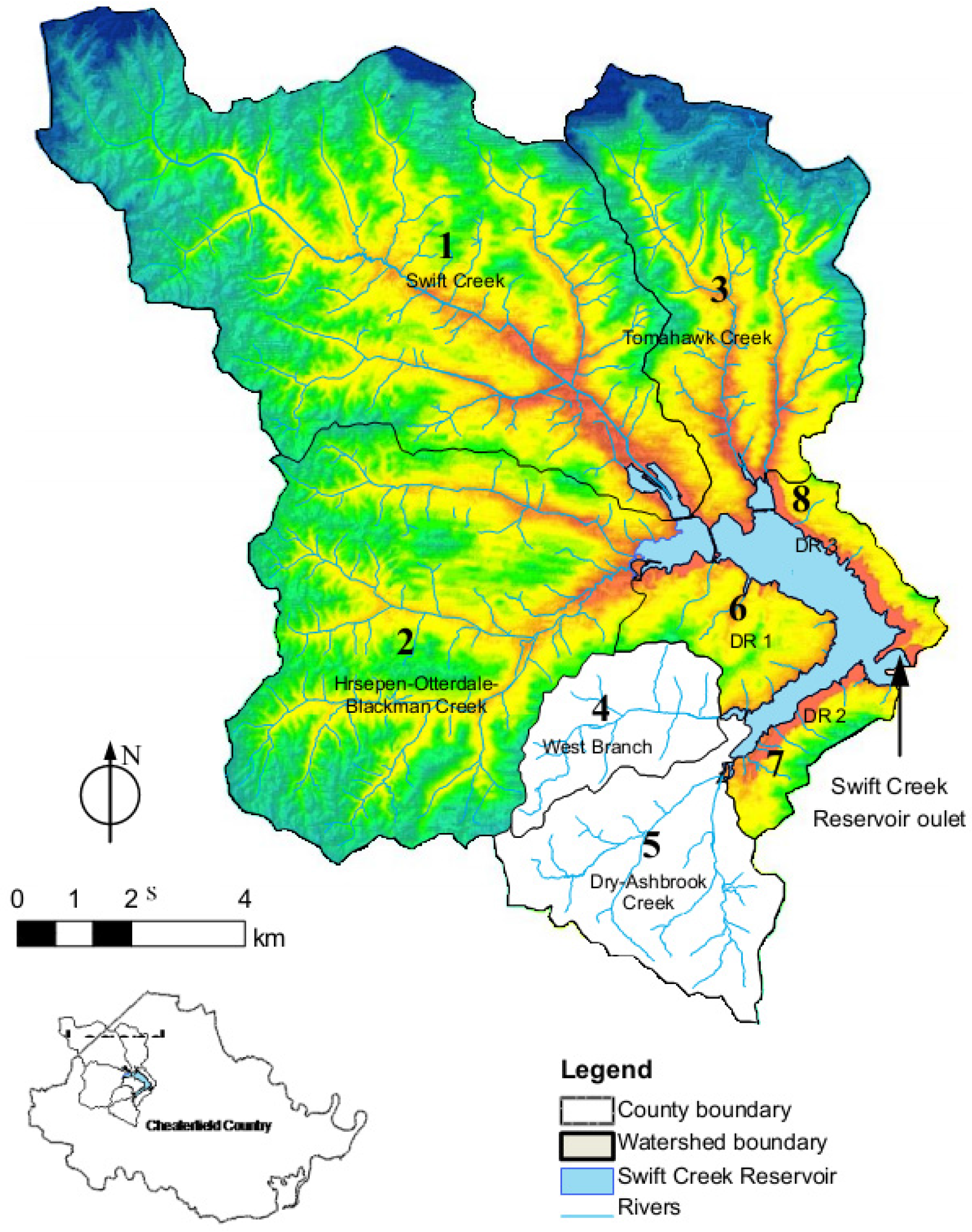
2.2. Application to the Swift Creek Reservoir Watershed

The Swift Creek Reservoir (SCR) Watershed is located in the Chesterfield County, VA, the United Sates (37.4° N, 77.7° W, 165 km²; Figure 1). Its major environmental concerns are algal blooms and hypolimnetic hypoxia in summer, the majority caused by two stressors: the loadings of inorganic nitrogen (NO₃⁻ and NH₄⁺) and inorganic phosphorus (PO₄³⁻) from eight sub-watersheds [28]. A hydrodynamic and water-quality model, CE-QUAL-W2 v3.1, was developed to represent such stressor-response relationships from 1998–2000 [28]. Previously, a nutrient TMDL allocation for the SCR watershed was developed through a stochastic simulation method by stochastically changing the pollutant removal rates among nonpoint sources from the eight sub-watersheds [15,18,28]. In our study, we applied the proposed BRRT-EILP model to determine optimal nutrient TMDL allocation under uncertainty for the SCR watershed. The goal of such TMDL allocation was to identify the critical load reductions from the eight sub-watersheds for the maintenance of summer (June–September) maxima of vertically averaged chlorophyll-a (Chl-a) concentrations at the reservoir outlet (defined as $y^{*\pm }$) below Chl-a criteria. According to Equations (1) and (2), the minimum total load reduction model for inorganic phosphorus and nitrogen for the SCR watershed could be formulated as follows:

$$Min{Z}^{\pm }={\displaystyle \sum _j^n\mathsf{\varphi }{\mathsf{\omega }}_{j1}{c}_{j1}^{\pm }{x}_{j1}^{\pm }}+{\displaystyle \sum _j^n(1-\mathsf{\varphi }){\mathsf{\omega }}_{j2}{c}_{j2}^{\pm }{x}_{j2}^{\pm }}$$

(3a)

$$s.t{y}^{ik\pm }={\mathsf{\beta }}_0^{ik}+{\displaystyle \sum _l^L{\displaystyle \sum _j^J{\mathsf{\beta }}_{jl}^{ik}{x}_{jl}^{\pm }}}\pm {\mathsf{\epsilon }}_{\mathsf{\alpha }}^{ik}\le y^{*\pm },\text{ for }{x}_{jl}^{\pm }\in [d_{jl}^{i-},d_{jl}^{i+}],\forall i,k$$

(3b)

$$x_{jl}^{\pm }\le x_l^{max},\forall j,l,x_{jl}^{\pm }\ge x_l^{min},\forall j,l,x_{jl}^{\pm },{\mathsf{\omega }}_j,c_{jl}^{\pm },y^{*\pm },x_{jl}^{min\pm }\ge 0$$

(3c)

where i represents the index of interval linear regression equations generated by the calibrated BRRT model, i = 1,2,…,I, I = 107, j is the index of the sub-watershed, j = 1,2,…,J, J = 8, k is the index of the compliance point, k = 1,2,…,K, K = 1 (reservoir outlet), and l is the index of the pollutant, l = 1, L, L = 2 (inorganic phosphorus and nitrogen). $Z^{\pm }$ is the total load reduction of inorganic phosphorus from the eight sub-watersheds when ϕ = 1 or the total load reduction of inorganic nitrogen from the eight sub-watersheds when ϕ = 0. ${\mathsf{\omega }}_{jl}$ is the weight for pollutant l from sub-watershed j that accounted for the relative difficulty or cost of the load reduction; whereas ${\mathsf{\omega }}_{jl}$ was assumed to be equal to 1.0 for all of the sub-watersheds, since no cost information from the previous best management practices (BMPs) implementation was available. $x_{jl}^{\pm }$ is the pollutant removal rate for pollutant l from sub-watershed j, calculated as the difference between baseline loadings (Table 1) and maximum allowable loadings (A_jl) at river mouths divided by baseline loadings, that is $x_{jl}^{\pm }=(c_{jl}^{\pm }-A_{jl}^{\pm })/c_{jl}^{\pm }$, where $c_{jl}^{\pm }$ is the baseline load of pollutant l in sub-watershed j, computed using Hydrological Simulation Program—FORTRAN (HSPF) v11 for the period from January–December 1998 (Table 1) [18]. ${\mathsf{\beta }}_{jl}^{ik}$ (including ${\mathsf{\beta }}_0^{ik}$) and ${\mathsf{\epsilon }}_{\mathsf{\alpha }}^{ik}$ are the regression coefficients and predictive error of the i-th interval linear regression equation at compliance point k, respectively. To derive the interval linear regression equations, the CE-QUAL-W2 v3.1 generated the simulated Chl-a (defined as $y^{ik\pm }$) with randomly-generated pollutant removal rates from 8 sub-watersheds, resulting in 2000 stressor-response datasets. We then calibrated these coefficients and determined the associated confidence intervals using BRRT v2. Since no Chl-a criteria have been published by either the United States Environmental Protection Agency or the State of Virginia, $y^{*\pm }$ was set at 12−15 μg/L in this study based on North Carolina water-quality standards and other references [28,29]. Three Chl-a criteria scenarios had been set as [12, 15], [13, 15] and [14, 15] μg/L; $x_l^{max}$ is the maximum removal level of the BMPs’ performance for pollutant l, which was set at 80% according to the American Society of Civil Engineers’ (ASCE) national BMP database; $x_l^{min}$ was set as zero, indicating that no nutrient load was removed; $d_{jl}^{i-}\in D^{i-}$, $d_{jl}^{i+}\in D^{i+}$.

Figure 1. Swift Creek Reservoir watershed and its eight sub-watersheds.

Figure 1. Swift Creek Reservoir watershed and its eight sub-watersheds.

Table 1. Baseline loadings (inorganic phosphorus and inorganic nitrogen) of Swift Creek Reservoir watershed.

Sub-Watershed j	Area, km2	ci1, kg	ci2, kg
1. Swift Creek	59.47	4451.7	157.4
2. Horsepen-Otterdale-Blackman Creek	40.47	5169.3	388.4
3. Tomahawk Creek	25.30	2677.2	126.8
4. West Branch	7.50	286.7	87.9
5. Dry-Ashbrook Creek	14.52	516.5	161.1
6. Direct runoff (1)	3.73	1916.3	114.2
7. Direct runoff (2)	6.13	1000.7	90.2
8. Direct runoff (3)	3.31	471.7	146.1
Total	160.4	16,490	1272

Table 1. Baseline loadings (inorganic phosphorus and inorganic nitrogen) of Swift Creek Reservoir watershed.

Sub-Watershed j	Area, km2	ci1, kg	ci2, kg
1. Swift Creek	59.47	4451.7	157.4
2. Horsepen-Otterdale-Blackman Creek	40.47	5169.3	388.4
3. Tomahawk Creek	25.30	2677.2	126.8
4. West Branch	7.50	286.7	87.9
5. Dry-Ashbrook Creek	14.52	516.5	161.1
6. Direct runoff (1)	3.73	1916.3	114.2
7. Direct runoff (2)	6.13	1000.7	90.2
8. Direct runoff (3)	3.31	471.7	146.1
Total	160.4	16,490	1272

2.3. Algorithmic Processes

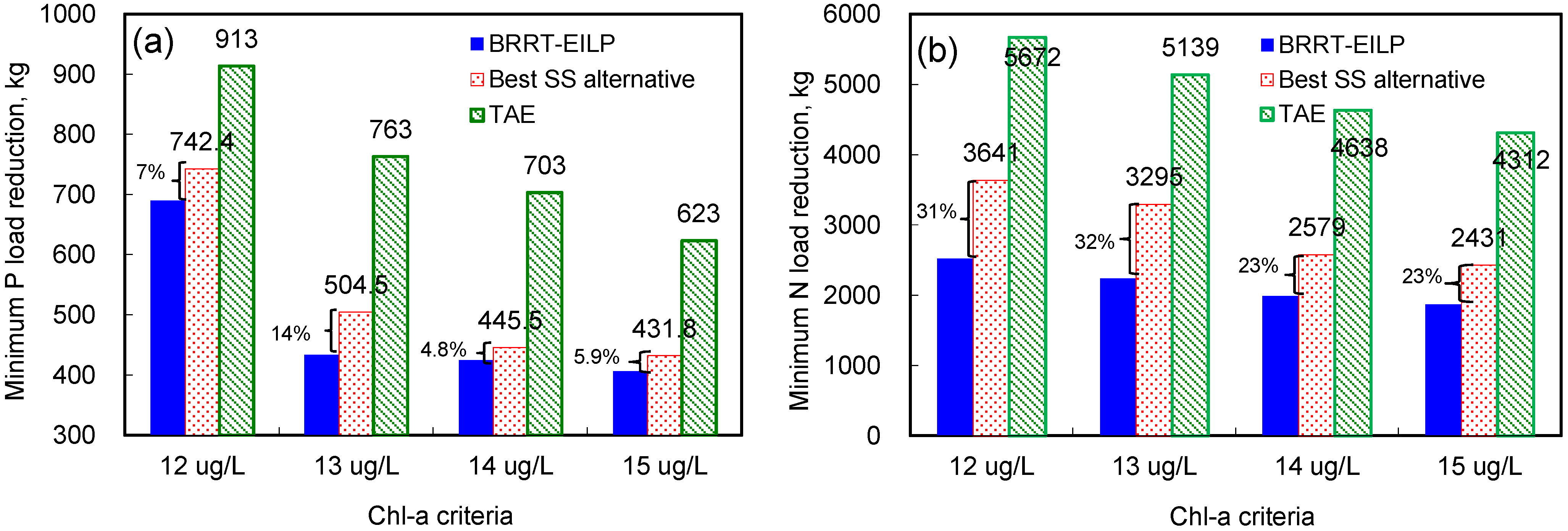
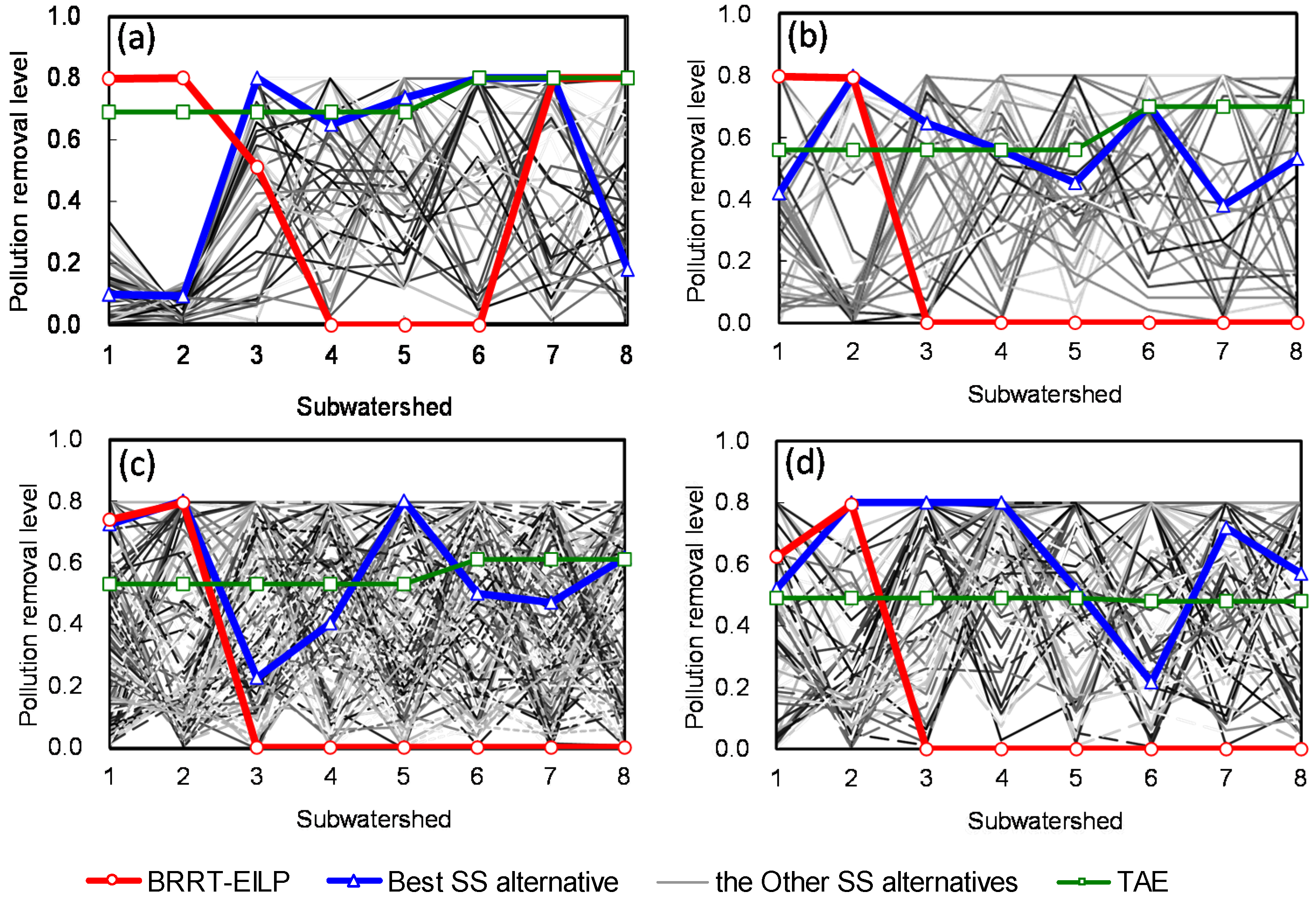
In order to explain our model in a logical and comprehensive way, we simply introduced the algorithmic processes of the BRRT-EILP model for determining optimal TMDL allocation under uncertainty.

Step 1: Generate the pollutant removal rates for pollution sources and simulate their responses at the compliance points using the water quality model, which results in a stressor-response dataset;

Step 2: Derive the interval linear regression equations by the BRRT v2 based on the stressor-response dataset (Figure 2);

Step 3: Formulate the minimum load reduction model (Equation (3)) under uncertainty by integrating interval linear regression equations into the EILP model;

Step 4: Following the EILP algorithm, solve the lower bound $Z^{-}$ (supplementary information, Text S2, Equation (S12a)) subject to constraints (supplementary information, Text S2, Equation (S13)), where the optimal pollutant removal rates are $x_{jopt}^{-}$ for j = 1, 2,…, k and $x_{jopt}^{+}$ for j = k + 1, k + 2,…, n and $Z_{opt}^{-}$; n is the number of x_j;

Step 5: Formulate the extra constraints ($x_j^{+}\ge x_{jopt}^{-}$ for j = 1, 2,…, k, $x_j^{-}\le x_{jopt}^{+}$ for j = k + 1, k + 2,…, n; see supplementary information, Text S2, Equations (S14b), (S14c) and (S15)) to ensure that the optimal pollutant removal rates $x_{opt}^{\pm }$ are absolutely feasible;

Step 6: Solve the upper bound $Z^{\text{+}}$ (supplementary information, Text S2, Equation (12b)) with its relevant and extra constraints (supplementary information, Text S2, Equations (S14) and (S15)), resulting in $Z_{opt}^{\pm }$, $E[Z_{opt}^{\pm }]$ and $X_{opt}^{\pm }=\left\{x_{opt}^{\pm }=[x_{jopt}^{-},x_{jopt}^{+}]|\forall j=1,2,\dots ,n\right\}$;

Step 7: Generate a set of pollutant removal rates or TMDL allocations under different risk levels according to the obtained optimal solutions $Z_{opt}^{\pm }$, $E[Z_{opt}^{\pm }]$, and $X_{opt}^{\pm }$. Analysis of these alternatives could allow acquiring both extreme and non-extreme TMDL allocations [15].

Figure 2. Algorithmic process for solving Bayesian recursive regression tree (BRRT)-enhanced-interval linear programming (EILP) model for risk-based optimal total maximum daily load (TMDL) allocation.

Figure 2. Algorithmic process for solving Bayesian recursive regression tree (BRRT)-enhanced-interval linear programming (EILP) model for risk-based optimal total maximum daily load (TMDL) allocation.

3. Results

Figure S1a,b demonstrates that the calibrated interval linear regression equations have low biases with large coefficients of determination (0.99 for calibration and 0.97 for validation), small mean squared errors (0.105 and 0.496 μg/L) and Bayesian information criteria (−3270 and −1592). This suggests that these equations could serve as a reliable approximation function of the complex CE-QUAL-W2 v3.1 model in accurately predicting the nonlinear effects of nitrogen and phosphorous loadings on the phytoplankton response (Figure S2). Note that the detailed results of calibration and cross-validation processes are presented in supplementary information Figure S1. Additionally, the calibrated interval linear regression equations were also verified by independent observations of summer maximum vertically averaged Chl-a concentrations at the reservoir outlet from 2004–2013. These data were obtained from Swift Creek Reservoir Reports. Although the 10-year observations are limited, the result of the verification process indicated that the calibrated interval linear regression equations could still reasonably capture the temporal variations of the summer maximum vertically-averaged Chl-a concentration (R² = 0.73; Figure S1c).

The results of the BRRT-EILP model show that the optimal required load reductions of inorganic nitrogen (ϕ = 1) from Swift Creek were 1870 kg/year under three scenarios (Table 2), while those from Dry-Ashbrook Creek greatly increased from [0, 120] in Scenario 1 to [0, 360] and [0, 413] kg/year in Scenarios 2 and 3, respectively. Additionally, Direct Runoff (1), from one of the sub-watersheds nearest to the compliance point, was required to reduce inorganic nitrogen by [0, 238] kg/year in Scenario 3. Consequently, the total inorganic nitrogen load reductions were [1870, 1989], [1870, 2235] and [1870, 2521] kg/year, respectively. The corresponding expected values were 1929.5, 2052.5 and 2195.5 kg/year.

The optimal solutions for the inorganic phosphorus load reductions (ϕ = 0) in Scenarios 1 and 2 indicate that it is necessary to reduce inorganic phosphorus loading only in the Swift Creek and Horsepen-Otterdale-Blackman (HOB) Creek sub-watersheds to reach a target Chl-a level of between 13 and 15 μg/L, with corresponding pollutant removal rates of [0.62, 0.74] and [0.62, 0.8] in the Swift Creek sub-watershed and 0.79 in the HOB Creek sub-watershed (Table 2). The total load reduction of inorganic phosphorus in Scenario 1 was [406.2, 424.2] kg/year, which is less than the optimal solution in Scenario 2 of [406.2, 433.6] kg/year. The expected load reduction values $E[Z_{opt}^{\pm }]$ in Scenarios 1 and 2 were 415.2 and 419.9 kg/year, respectively. In Scenario 3 ($c^{\pm }=[12,15]$ μg/L), the required inorganic phosphorus load reduction from HOB Creek was slightly increased to [308, 310.8] kg compared to the Scenario 2 requirement of 308 kg/y. In addition, the Tomahawk Creek, Direct Runoff (2) and Direct Runoff (3) sub-watersheds were required to reduce inorganic phosphorus by [0, 64.8], [0, 72.2] and [0, 116.9] kg/year, respectively. Together, the total load reduction and its expected values $E[Z_{opt}^{\pm }]$ in Scenario 3 were [406.2, 690.2] and 548.2 kg/year respectively.

Based on these optimal reductions under different Chl-a criteria levels (i.e., 12, 13, 14, 15 μg/L), vertically-averaged Chl-a concentrations at the reservoir outlet were further simulated and verified by CE-QUAL-W2 v3.1. The results in Figure S2 indicated that the maximum Chl-a concentrations of all optimal solutions were almost identical to the simulation results, which further confirmed the predictive accuracy of BRRT-derived interval linear regression equations.

Table 2. Optimal pollution removal levels of inorganic phosphorus and inorganic nitrogen for the Swift Creek Reservoir (SCR) watershed for three scenarios.

Sub-watershed j

Minimum Total Load Reduction of Inorganic Nitrogen

Minimum Total Load Reduction of Inorganic Phosphorus

Scenario 1 (Chl-a: [14, 15] μg/L)

Scenario 2 (Chl-a: [13, 15] μg/L)

Scenario 3 (Chl-a: [12, 15] μg/L)

Scenario 1

Scenario 2

Scenario 3

$x_{j1}^{\pm }$ *

$c_{j1}^{\pm }{x}_{j1}^{\pm }$ *, kg

$x_{j1}^{\pm }$

$c_{j1}^{\pm }{x}_{j1}^{\pm }$, kg

$x_{j1}^{\pm }$

$c_{j1}^{\pm }{x}_{j1}^{\pm }$, kg

$x_{j2}^{\pm }$

$c_{j2}^{\pm }{x}_{j2}^{\pm }$, kg

$x_{j2}^{\pm }$

$c_{j2}^{\pm }{x}_{j2}^{\pm }$, kg

$x_{j2}^{\pm }$

$c_{j2}^{\pm }{x}_{j2}^{\pm }$, kg

1

[0.42, 0.42]

[1870, 1870]

[0.42, 0.42]

[1870, 1870]

[0.42, 0.42]

[1870, 1870]

[0.62, 0.74]

[98.2, 116.2]

[0.62, 0.8]

[98.2, 125.6]

[0.62, 0.8]

[98.2, 125.6]

2

[0, 0]

[0, 0]

[0, 0]

[0, 0]

[0, 0]

[0, 0]

[0.79, 0.79]

[308, 308]

[0.79, 0.79]

[308, 308]

[0.79, 0.8]

[308, 310.7]

3

[0, 0]

[0, 0]

[0, 0]

[0, 0]

[0, 0]

[0, 0]

[0, 0]

[0, 0]

[0, 0]

[0, 0]

[0, 0.51]

[0, 64.8]

4

[0, 0]

[0, 0]

[0, 0]

[0, 0]

[0, 0]

[0, 0]

[0, 0]

[0, 0]

[0, 0]

[0, 0]

[0, 0]

[0, 0]

5

[0, 0.23]

[0, 120]

[0, 0.71]

[0, 360]

[0, 0.8]

[0, 413]

[0, 0]

[0, 0]

[0, 0]

[0, 0]

[0, 0]

[0, 0]

6

[0, 0]

[0, 0]

[0, 0]

[0, 0]

[0, 0.12]

[0, 238]

[0, 0]

[0, 0]

[0, 0]

[0, 0]

[0, 0]

[0, 0]

7

[0, 0]

[0, 0]

[0, 0]

[0, 0]

[0, 0]

[0, 0]

[0, 0]

[0, 0]

[0, 0]

[0, 0]

[0, 0.8]

[0, 72.2]

8

[0, 0]

[0, 0]

[0, 0]

[0, 0]

[0, 0]

[0, 0]

[0, 0]

[0, 0]

[0, 0]

[0, 0]

[0, 0.8]

[0, 116.9]

Total load reduction

[1870, 1989]

[1870, 2235]

[1870, 2521]

[406.2, 424.2]

[406.2, 433.6]

[406.2, 690.2]

$E[Z_{opt}^{\pm }]$

1929.5

2052.5

2195.5

415.2

419.9

548.2

Notes: * $x_{j1}^{\pm }$ is the removal rate of pollutant l (l = 1: inorganic nitrogen, l = 2: inorganic phosphorus) in sub-watershed j; $c_{j1}^{\pm }$ is the baseline load; $c_{j1}^{\pm }{x}_{j1}^{\pm }$ is the pollutant removal amount for pollutant l from sub-watershed j.

Table 2. Optimal pollution removal levels of inorganic phosphorus and inorganic nitrogen for the Swift Creek Reservoir (SCR) watershed for three scenarios.

Sub-watershed j

Minimum Total Load Reduction of Inorganic Nitrogen

Minimum Total Load Reduction of Inorganic Phosphorus

Scenario 1 (Chl-a: [14, 15] μg/L)

Scenario 2 (Chl-a: [13, 15] μg/L)

Scenario 3 (Chl-a: [12, 15] μg/L)

Scenario 1

Scenario 2

Scenario 3

$x_{j1}^{\pm }$ *

$c_{j1}^{\pm }{x}_{j1}^{\pm }$ *, kg

$x_{j1}^{\pm }$

$c_{j1}^{\pm }{x}_{j1}^{\pm }$, kg

$x_{j1}^{\pm }$

$c_{j1}^{\pm }{x}_{j1}^{\pm }$, kg

$x_{j2}^{\pm }$

$c_{j2}^{\pm }{x}_{j2}^{\pm }$, kg

$x_{j2}^{\pm }$

$c_{j2}^{\pm }{x}_{j2}^{\pm }$, kg

$x_{j2}^{\pm }$

$c_{j2}^{\pm }{x}_{j2}^{\pm }$, kg

1

[0.42, 0.42]

[1870, 1870]

[0.42, 0.42]

[1870, 1870]

[0.42, 0.42]

[1870, 1870]

[0.62, 0.74]

[98.2, 116.2]

[0.62, 0.8]

[98.2, 125.6]

[0.62, 0.8]

[98.2, 125.6]

2

[0, 0]

[0, 0]

[0, 0]

[0, 0]

[0, 0]

[0, 0]

[0.79, 0.79]

[308, 308]

[0.79, 0.79]

[308, 308]

[0.79, 0.8]

[308, 310.7]

3

[0, 0]

[0, 0]

[0, 0]

[0, 0]

[0, 0]

[0, 0]

[0, 0]

[0, 0]

[0, 0]

[0, 0]

[0, 0.51]

[0, 64.8]

4

[0, 0]

[0, 0]

[0, 0]

[0, 0]

[0, 0]

[0, 0]

[0, 0]

[0, 0]

[0, 0]

[0, 0]

[0, 0]

[0, 0]

5

[0, 0.23]

[0, 120]

[0, 0.71]

[0, 360]

[0, 0.8]

[0, 413]

[0, 0]

[0, 0]

[0, 0]

[0, 0]

[0, 0]

[0, 0]

6

[0, 0]

[0, 0]

[0, 0]

[0, 0]

[0, 0.12]

[0, 238]

[0, 0]

[0, 0]

[0, 0]

[0, 0]

[0, 0]

[0, 0]

7

[0, 0]

[0, 0]

[0, 0]

[0, 0]

[0, 0]

[0, 0]

[0, 0]

[0, 0]

[0, 0]

[0, 0]

[0, 0.8]

[0, 72.2]

8

[0, 0]

[0, 0]

[0, 0]

[0, 0]

[0, 0]

[0, 0]

[0, 0]

[0, 0]

[0, 0]

[0, 0]

[0, 0.8]

[0, 116.9]

Total load reduction

[1870, 1989]

[1870, 2235]

[1870, 2521]

[406.2, 424.2]

[406.2, 433.6]

[406.2, 690.2]

$E[Z_{opt}^{\pm }]$

1929.5

2052.5

2195.5

415.2

419.9

548.2

Notes: * $x_{j1}^{\pm }$ is the removal rate of pollutant l (l = 1: inorganic nitrogen, l = 2: inorganic phosphorus) in sub-watershed j; $c_{j1}^{\pm }$ is the baseline load; $c_{j1}^{\pm }{x}_{j1}^{\pm }$ is the pollutant removal amount for pollutant l from sub-watershed j.

In simple terms, we used Scenario 3 ($c^{\pm }=[12,15]$ µg/L) for inorganic nitrogen as an example to illustrate the extreme and non-extreme tradeoffs between the benefits of TMDL allocation and the diverse risk levels of violating the constraints, and the results for the other two scenarios are shown in supplementary information, Text S3.

Minimum Total Load Reductions of Inorganic Nitrogen

(i) The first decision alternative in the extreme tradeoff analysis was $X_1=\left\{x_{jl}^{-}|x_{11opt}^{-}=\text{0.42};x_{j1opt}^{-}=0\text{ for other }j\right\}$ with the lowest total load reduction $Z_{opt}^{-}$ of 1870 kg of inorganic nitrogen. This corresponded to the highest risk level of violating the constraints.

(ii) The second decision alternative in the extreme tradeoff analysis was $X_2=\left\{x_{jl}^{+}|x_{11opt}^{+}=\text{0.42};x_{51opt}^{+}=\text{0.8;}{x}_{61opt}^{+}=\text{0.12;}{x}_{j1opt}^{+}=0\text{ for other }j\right\}$ with the highest total load reduction $Z_{opt}^{+}$ of 2521 kg of inorganic nitrogen, corresponding to the lowest risk level of violating the constraints.

(iii) The third decision alternative in the non-extreme tradeoff analysis was $X_3=\{x_{jl}^{\pm }|{\displaystyle \sum _j^8{c}_{jl}^{\pm }{x}_{jl}^{\pm }}=2195.5\text{ where }{x}_{11opt}^{\pm }=0.42;x_{51opt}^{\pm }=[0,\text{0.8];}{x}_{61opt}^{\pm }=[0,\text{0.12] and }$ $x_{j1opt}^{\pm }=0\text{ for other }j\}$ with an expected value of total load reduction $E[Z_{opt}^{\pm }]$ of 2195.5 kg of inorganic nitrogen, corresponding to a moderate risk level of violating the constraints.

4. Discussion

The optimal results in Table 2 suggest that the Swift Creek sub-watershed contributes more than 3/4 to the total nitrogen load reductions under different scenarios, though its per-area nitrogen loading ranked third from bottom (Table 1). Nevertheless, low per-area nitrogen loading does not mean that the nitrogen concentrations at the outlet of Swift Creek are lower than the other sub-watersheds. Actually, both nitrogen concentrations in this sub-watershed are highest within the simulation period [28] compared to the others. Such worse water quality is primarily caused by the urban pollution sources, such as domestic sewage and urban storm water, rather than the agricultural pollution source loss via surface runoff [28]. Additionally, both the nitrogen and phosphorous load reductions are required largely in the Swift Creek sub-watershed. Such a result is determined through the optimization processes by the BRRT-EILP model, which assigns a higher pollutant removal rate to the sub-watershed where the Chl-a concentration is more sensitive to the increase of load reductions. We believe that the large load reductions of both pollutants are reasonable when only considering the efficiency criteria in the optimization process, as there exists a synergy between nitrogen and phosphorous load reductions within wastewater treatment plants (WWTPs). When decision makers are interested in knowing the optimal TMDL allocation in cases where the total cost is to be minimized or the equitability among stakeholders is met, the objective functions and the associated constraints can be easily revised.

The computational cost of the BRRT-EILP model was significantly lower than that of conventional global optimization algorithms, such as genetic algorithms, evolutionary algorithms and simulated annealing (Table 3). The major computation time for the BRRT-EILP method was in the generation of the stressor-response dataset for calibrating and verifying the linear regression equations, which approximately took 2000 min, as it takes around 1 min for an Intel^® Core™ 2 Duo 2.4-GHz computer (CPU T8300) to complete one CE-QUAL-W2 model run. Other than that, the calibration and verification of the BRRT model takes only about 5 min, and finding the optimal solution of the BRRT-EILP model for three scenarios with 16 decision variables takes less than 1 min. Taken together, the total computational time taken to find out the approximate optimal solutions was only about 33 h. In contrast, running a traditional direct SOM framework using a GA approach might require several days (e.g., if a population size of 50 is used and the model is iterated for 300 generations, it takes over 10 days to obtain a solution) [11]. More time would be required to increase the chances of obtaining globally-approximate optimal solutions, because multiple GA runs would need to be executed for the same problem [21,22]. Moreover, the computation efficiency of the proposed BRRT-EILP model can be significantly higher than that of the traditional direct SOM approach when Equation (3) is used to evaluate solutions for different objective functions, water-quality criteria or system constraints. For example, assume that decision makers are interested in the optimal TMDL allocation in cases where the total cost, rather than the total reduction level, is to be minimized, or when water quality targets for dissolved oxygen are also considered, or when they are interested in achieving compliance at more than one location. In such cases, traditional direct SOM would involve re-running the stochastic search algorithm, which is very inefficient and can be computationally prohibitive if many scenarios need to be analyzed. In contrast, the BRRT-EILP model would require less than 1 min to compute such a new scenario, since it is not necessary to repeat the time-consuming data generation process required for BRRT calibration/verification in the scenario analysis stage.

Table 3. Method comparison of computational cost.

Method	Calibration	New Application
BRRT-EILP model	33 h	1 min
Direct SOM framework	~10 days	~10 days

Table 3. Method comparison of computational cost.

Method	Calibration	New Application
BRRT-EILP model	33 h	1 min
Direct SOM framework	~10 days	~10 days

The advantage of applying the BRRT-EILP model in place of stochastic simulation and TAE methods for TMDL development can be demonstrated by comparing the allocations resulting from each of the methods. First, 4000 scenarios were generated by randomly changing the inorganic nitrogen or inorganic phosphorus removal rates (no more than 80%) from eight sub-watersheds. The alternative where the sum of load reductions is minimum is eventually selected as the best allocation. Figure 3 shows that the alternatives of 3.6, 3.3, 2.6 and 2.4 × 10³ tonnes were identified as feasible inorganic nitrogen load reductions to meet Chl-a maximum criteria of 12, 13, 14 and 15 μg/L, respectively. Additionally, alternatives of 0.74, 0.50, 0.44 and 0.43 × 10³ tonnes were identified as feasible load reductions for inorganic phosphorus. Second, a TAE analysis of inorganic nitrogen or phosphorus load reduction was conducted by iteratively reducing loads using different reduction ratios for different sub-watersheds. In this case, we first implemented the load reductions for the three sub-watersheds (Direct Runoff (1)–(3)) closest to the outlet until a certain pre-specified maximum achievable reduction ratio was reached and then reduced loads from the five upstream sub-watersheds until compliance with Chl-a criteria was achieved in the three scenarios. The minimum load reductions identified by the TAE method (4.3–5.7 × 10³ tonnes for inorganic nitrogen, 0.62–0.91 × 10³ tonnes for phosphorus inorganic) are much larger than those of the BRRT-EILP method. Figure 3, Figure 4 and Figure 5 show the minimum load reductions and pollution removal levels of the BRRT-EILP model compared to those of the two kinds of feasible alternatives generated by stochastic simulation and TAE methods. Specifically, the minimum inorganic phosphorus load reductions derived by the BRRT-EILP model were 7.0%, 14%, 4.8% and 5.9% less than those of the best stochastic simulation (SS) alternatives when the Chl-a criteria were levels below 12, 13, 14 and 15 μg/L, respectively (Figure 3a). The SS method required reducing inorganic phosphorus loads in all eight of the sub-watersheds, while the BRRT-EILP model required reductions in no more than five sub-watersheds (Figure 4). The reductions of inorganic nitrogen loads required by the BRRT-EILP solutions were 31%, 32%, 23% and 23% less than those of the best SS alternatives (Figure 3b). Additionally, the BRRT-EILP solutions only required inorganic nitrogen pollution removal in Swift Creek, Dry-Ashbrook Creek and Direct Runoff (1), while the removal rates of best SS alternatives required reductions greater than 0.3 in Sub-watersheds 1, 4, 5 and 8 (Figure 5). The plausible explanation for such sub-watershed selection by BRRT-EILP model is that the summer maximum vertically-averaged Chl-a concentration is more sensitive to load reductions in the selected sub-watersheds than the others. Another possible explanation is that the SS method uses random search, rather than the heuristic search applied by the BRRT-EILP model. In addition, the BRRT-EILP solutions were superior to those of the TAE method, since the latter ignores the difference in the sensitivity of Chl-a concentration to a unit of incremental load reduction across different sub-watersheds, while the BRRT-EILP model could rapidly identify critical sub-watersheds, resulting in the approximately most effective and reliable TMDL allocation. Therefore, the BRRT-EILP model may provide a new framework for updating the current TMDL allocation paradigm.

Figure 3. Minimum load reductions of the BRRT-EILP model, best stochastic simulation (SS) alternatives and trial-and-error (TAE) solutions that meet Chl-a criteria below 12, 13, 14 and 15 μg/L. (a) Inorganic phosphorus; (b) inorganic nitrogen. The percentage in the panels is calculated as the difference in minimum load reductions between the BRRT-EILP model and the SS method divided by that of the SS method.

Figure 3. Minimum load reductions of the BRRT-EILP model, best stochastic simulation (SS) alternatives and trial-and-error (TAE) solutions that meet Chl-a criteria below 12, 13, 14 and 15 μg/L. (a) Inorganic phosphorus; (b) inorganic nitrogen. The percentage in the panels is calculated as the difference in minimum load reductions between the BRRT-EILP model and the SS method divided by that of the SS method.

Figure 4. Pollution removal levels of inorganic phosphorus solved by the BRRT-EILP model, best stochastic simulation (SS) alternatives and the TAE method that meet diverse Chl-a criteria. (a) Chl-a = 12 μg/L; (b) Chl-a = 13 μg/L; (c) Chl-a = 14 μg/L and (d) Chl-a = 15 μg/L. The red, blue and green solid lines indicate the solutions of the BRRT-EILP model, the best stochastic simulation (SS) alternatives and the TAE method, while the other lines (in gray) represent the other alternatives with the SS method.

Figure 4. Pollution removal levels of inorganic phosphorus solved by the BRRT-EILP model, best stochastic simulation (SS) alternatives and the TAE method that meet diverse Chl-a criteria. (a) Chl-a = 12 μg/L; (b) Chl-a = 13 μg/L; (c) Chl-a = 14 μg/L and (d) Chl-a = 15 μg/L. The red, blue and green solid lines indicate the solutions of the BRRT-EILP model, the best stochastic simulation (SS) alternatives and the TAE method, while the other lines (in gray) represent the other alternatives with the SS method.

Figure 5. Pollution removal levels of inorganic nitrogen solved by the BRRT-EILP model and the TAE simulation method that meet diverse Chl-a criteria. (a) Chl-a = 12 μg/L; (b) Chl-a = 13 μg/L; (c) Chl-a = 14 μg/L and (d) Chl-a = 15 μg/L. The meaning of the colors is the same as in Figure 4.

Figure 5. Pollution removal levels of inorganic nitrogen solved by the BRRT-EILP model and the TAE simulation method that meet diverse Chl-a criteria. (a) Chl-a = 12 μg/L; (b) Chl-a = 13 μg/L; (c) Chl-a = 14 μg/L and (d) Chl-a = 15 μg/L. The meaning of the colors is the same as in Figure 4.

Another advantage of the BRRT-EILP model is that it could provide extreme and non-extreme tradeoff analyses under uncertainty, which divides the solution space of $X_{opt}^{+}$ based on the different risk levels of parameters. Three decision alternatives ($Z_{opt}^{-}$, $Z_{opt}^{+}$ and $E[Z_{opt}^{\pm }]$) could be generated corresponding to the different risk levels on both the left-hand ($y^{ik\pm }$) and right-hand ($y^{*\pm }$) sides. Although the risk level could not be completely quantified, since the probability density functions of all enhanced-interval numbers were not easy to determine, the three decision alternatives with their qualitative risk levels for violating constraints represented a series of system performances of load reductions for decision makers who have a diverse tolerance of risk levels.

The optimized annual inorganic nitrogen and phosphorous load reductions could be further translated as the allowable nutrient TMDL equivalent, including individual waste load allocations (WLAs) for point sources and load allocations (LAs) for nonpoint sources. Although the permit condition in this study is written to ensure attainment of these load allocations as annual averages, it may be translated into ordinary discharge limitations with the associated risk levels. First, we suggest determining the potential load reduction by assessing the effectiveness of supporting additional BMPs for agriculture, followed by the assignment of different risk levels to account for the uncertainties of the optimal results. The sum of the WLAs needed to meet the TMDL is then calculated: ∑WLAs = TMDL − LAs. The next step is to translate WLAs into permits as discharge limitations. According to the USEPA guidelines [30], discharge limitations may be expressed either as numerical restrictions for continuous discharges or as average weekly and average monthly discharge limitations for WWTPs and as daily maximums and monthly averages for other dischargers, which is an additional step that can be taken in the future.

5. Conclusions

In this study, we developed a BRRT-EILP model to serve as an indirect SOM framework for risk-based optimal TMDL allocation. The proposed method was applied to the real-world case of the SCR watershed, and the results indicated that the BRRT-EILP model is computationally efficient and capable of risk-based decision making for TMDL allocation under uncertainty. The main conclusions are that:

(i) The interval linear regression equations derived from the BRRT approach accurately approximated the nonlinear stressor-response relationships represented in a sophisticated water quality model. The resulting BRRT-EILP optimization framework derived from interval linear regression equations could serve as an efficient decision support tool that overcomes the computational bottleneck from traditional direct SOM framework.

(ii) The BRRT-EILP model can be efficiently solved and easily acquire approximate optimal solutions at various risk levels. Furthermore, the solutions obtained from BRRT-EILP model could significantly improve TMDL allocations and the associated tradeoff analysis compared to the ones obtained by traditional stochastic simulation and TAE approaches.

(iii) Although the BRRT-EILP model was first proposed for nutrient TMDL allocation to mitigate harmful algal blooms in a reservoir, recent studies suggest that this model and its solution algorithm could also possibly be applied to new critical problems, like hypoxia [5,31] and heavy metals in other nonlinear aquatic systems under uncertainty. In particular, the objective function Equation (2a) could take various forms, including measures of reliability and equity, and the system constraints of Equation (2b)–(2e) could be modified to ensure compliance with both dissolved oxygen and heavy metal criteria. Nevertheless, the BRRT-derived equivalent needs to be further derived from a process-based model and verified by field data prior to its application in decision making.

References

1. USEPA. Allocating Loads and Wasteloads, Technical Support Documents, Total Maximum Daily Load (TMDL); US EPA Press: Washington, DC, USA, 2003.
2. Jia, Y.B.; Culver, T.B. Robust optimization for total maximum daily load allocations. Water Resour. Res. 2006, 42. [Google Scholar] [CrossRef]
3. Cerco, C.F.; Noel, M.R.; Kim, S.C. Three-dimensional management model for lake washington, part ii: Eutrophication modeling and skill assessment. Lake Reserv. Manag. 2006, 22, 115–131. [Google Scholar] [CrossRef]
4. Cole, T.; Wells, S.A. CE-QUAL-W2: A Two-Dimensional, Laterally Averaged, Hydrodynamic and Water Quality Model, Version 3.1; US Army Engineering and Research Development Center: Vicksburg, MS, USA, 2003. [Google Scholar]
5. Boesch, D.F. The gulf of Mexico’s dead zone. Science 2004, 306, 977–978. [Google Scholar] [CrossRef]
6. Dhar, A.; Datta, B. Optimal operation of reservoirs for downstream water quality control using linked simulation optimization. Hydrol. Process. 2008, 22, 842–853. [Google Scholar] [CrossRef]
7. He, L.; Huang, G.H.; Lu, H.W. Health-risk-based groundwater remediation system optimization through clusterwise linear regression. Environ. Sci. Technol. 2008, 42, 9237–9243. [Google Scholar] [CrossRef] [PubMed]
8. He, L.; Huang, G.H.; Zeng, G.M.; Lu, H.W. An integrated simulation, inference, and optimization method for identifying groundwater remediation strategies at petroleum-contaminated aquifers in western canada. Water Res. 2008, 42, 2629–2639. [Google Scholar] [CrossRef]
9. Huang, G.H.; Huang, Y.F.; Wang, G.Q.; Xiao, H.N. Development of a forecasting system for supporting remediation design and process control based on NAPL-biodegradation simulation and stepwise-cluster analysis. Water Resour. Res. 2006, 42. [Google Scholar] [CrossRef]
10. Rejani, R.; Jha, M.K.; Panda, S.N. Simulation-optimization modelling for sustainable groundwater management in a coastal basin of orissa, india. Water Resour. Manag. 2009, 23, 235–263. [Google Scholar] [CrossRef]
11. Saadatpour, M.; Afshar, A. Waste load allocation modeling with fuzzy goals; simulation-optimization approach. Water Resour. Manag. 2007, 21, 1207–1224. [Google Scholar] [CrossRef]
12. Zhou, F.; Chen, G.X.; Huang, Y.F.; Yang, J.Z.; Feng, H. An adaptive moving finite volume scheme for modeling flood inundation over dry and complex topography. Water Resour. Res. 2013, 49, 1914–1928. [Google Scholar] [CrossRef]
13. Zhou, F.; Chen, G.X.; Noelle, S.; Guo, H.C. A well-balanced stable generalized riemann problem scheme for shallow water equations using adaptive moving unstructured triangular meshes. Int. J. Numer. Methods Fluids 2013, 73, 266–283. [Google Scholar] [CrossRef]
14. Qin, X.S.; Huang, G.H.; Chakma, A. A stepwise-inference-based optimization system for supporting remediation of petroleum-contaminated sites. Water Air Soil Pollut. 2007, 185, 349–368. [Google Scholar] [CrossRef]
15. Guo, H.C.; Gao, W.; Zhou, F. Three-level trade-off analysis for decision making in environmental engineering under interval uncertainty. Eng. Optim. 2014, 46, 377–392. [Google Scholar] [CrossRef]
16. Huang, G.H. A stepwise cluster-analysis method for predicting air-quality in an urban-environment. Atmos. Environ. B Urban Atmos. 1992, 26, 349–357. [Google Scholar] [CrossRef]
17. Sahinidis, N.V. Optimization under uncertainty: State-of-the-art and opportunities. Comput. Chem. Eng. 2004, 28, 971–983. [Google Scholar] [CrossRef]
18. Wang, Z.; Gao, W.; Cai, Y.L.; Guo, H.C.; Zhou, F. Joint optimization of population pattern and end-of-pipe control under uncertainty for lake dianchi water-quality management. Fresenius Environ. Bull. 2012, 21, 3693–3704. [Google Scholar]
19. Zhou, F.; Huang, G.H.; Chen, G.X.; Guo, H.C. Enhanced-interval linear programming. Eur. J. Oper. Res. 2009, 199, 323–333. [Google Scholar] [CrossRef]
20. Birge, J.R.; Louveaux, F.V. Introduction to Stochastic Programming; Springer: New York, NY, USA, 1997. [Google Scholar]
21. Zou, R.; Liu, Y.; Riverson, J.; Parker, A.; Carter, S. A nonlinearity interval mapping scheme for efficient waste load allocation simulation-optimization analysis. Water Resour. Res. 2010, 46. [Google Scholar] [CrossRef]
22. Zou, R.; Lung, W.S.; Wu, J. An adaptive neural network embedded genetic algorithm approach for inverse water quality modeling. Water Resour. Res. 2007, 43. [Google Scholar] [CrossRef]
23. Zhou, F.; Guo, H.C.; Chen, G.X.; Huang, G.H. The interval linear programming: A revisit. J. Environ. Inform. 2008, 11, 1–10. [Google Scholar] [CrossRef]
24. Iorgulescu, I.; Beven, K.J. Nonparametric direct mapping of rainfall-runoff relationships: An alternative approach to data analysis and modeling? Water Resour. Res. 2004, 40. [Google Scholar] [CrossRef]
25. Breiman, L.; Friedman, J.H.; Olshen, R.A.; Stone, C.G. Classification and Regression Trees; Wadsworth International Group: Belmont, CA, USA, 1984. [Google Scholar]
26. Zhou, F.; Shang, Z.Y.; Zeng, Z.Z.; Piao, S.L.; Ciais, P.; Raymond, P.; Wang, X.H.; Wang, R.; Chen, M.P.; Yang, C.L.; et al. New model for capturing the variations of fertilizer-induced emission factors of n2o. Glob. Biogeochem. Cycles 2015, 29. [Google Scholar] [CrossRef]
27. Harmel, R.D.; Cooper, R.J.; Slade, R.M.; Haney, R.L.; Arnold, J.G. Cumulative uncertainty in measured streamflow and water quality data for small watersheds. Trans. ASABE 2006, 49, 689–701. [Google Scholar] [CrossRef]
28. Wu, J.; Zou, R.; Yu, S.L. Uncertainty analysis for coupled watershed and water quality modeling systems. J. Water Resour. Plann. Manag. 2006, 132, 351–361. [Google Scholar] [CrossRef]
29. Wetzel, R.G. Limnology—Lake and River Ecosystems, 3rd ed.; Academic Press: New York, NY, USA, 2001. [Google Scholar]
30. U.S. Environmental Protection Agency (USEPA). Protocol for Developing Nutrient TMDLs; EPA 841-B-99-007; Office of Water (4503F), United States Environmental Protection Agency: Washington, DC, USA, 1999.
31. Conley, D.J.; Paerl, H.W.; Howarth, R.W.; Boesch, D.F.; Seitzinger, S.P.; Havens, K.E.; Lancelot, C.; Likens, G.E. Ecology controlling eutrophication: Nitrogen and phosphorus. Science 2009, 323, 1014–1015. [Google Scholar] [CrossRef]