Empirical Estimation of Total Nitrogen and Total Phosphorus Concentration of Urban Water Bodies in China Using High Resolution IKONOS Multispectral Imagery

Abstract

Measuring total nitrogen (TN) and total phosphorus (TP) is important in managing heavy polluted urban waters in China. This study uses high spatial resolution IKONOS imagery with four multispectral bands, which roughly correspond to Landsat/TM bands 1–4, to determine TN and TP in small urban rivers and lakes in China. By using Lake Cihu and the lower reaches of Wen-Rui Tang (WRT) River as examples, this paper develops both multiple linear regressions (MLR) and artificial neural network (ANN) models to estimate TN and TP concentrations from high spatial resolution remote sensing imagery and in situ water samples collected concurrently with overpassing satellite. The measured and estimated values of both MLR and ANN models are in good agreement (R² > 0.85 and RMSE < 2.50). The empirical equations selected by MLR are more straightforward, whereas the estimated accuracy using ANN model is better (R² > 0.86 and RMSE < 0.89). Results validate the potential of using high resolution IKONOS multispectral imagery to study the chemical states of small-sized urban water bodies. The spatial distribution maps of TN and TP concentrations generated by the ANN model can inform the decision makers of variations in water quality in Lake Cihu and lower reaches of WRT River. The approaches and equations developed in this study could be applied to other urban water bodies for water quality monitoring.

1. Introduction

Urbanization has become a ubiquitous global change over the 20th century [1]. As a “living laboratory” in urbanization [2], China has experienced rapid economic development and urbanization in the past three decades. Rapid urbanization in China has resulted in widespread surface water eutrophication and water quality degradation because of the lack of sanitation and uneven distribution of water treatment facilities compared to most developing countries [3]. The fact that 90% of urban waterways are classified as heavily polluted has raised great concerns about human and aquatic ecosystem health [4,5].

Monitoring water quality is the first step toward understanding the characteristics of water pollution and devising effective mitigation strategies. Traditionally, water quality parameters (WQPs), such as total nitrogen (TN) and total phosphorus (TP), are obtained by routine monitoring methods of field sampling and laboratory analyses [6]. In addition to cost and labor intensiveness, these traditional approaches are not suitable for monitoring a large number of water bodies at a regional or national scale because of spatial heterogeneity and temporal changes of water quality across aquatic ecosystems. This condition is especially true for urban lake and river systems, where numerous point and non-point inputs occur over relatively short distances [4]. With the constant development of environmental information technology, remote sensing plays an important and effective role in water quality monitoring because of its wider coverage, higher efficiency, and lower cost than traditional sampling methods. Sensors aboard satellites with a wide variety of spectral, spatial, and temporal resolutions have been used to access several water quality parameters. Because the optical properties of water depend on the concentration and character of total suspended sediments (TSS), phytoplankton (typically estimated by chlorophyll-a measurements), and chromophoric dissolved organic matter (CDOM), numerous studies, e.g. [7,8,9], have previously demonstrated the application of satellite remote sensing to monitor these three water quality parameters. Of all pollutants, nitrogen (N), which is needed for protein synthesis, and phosphorus (P), which is needed for DNA, RNA, and energy transfer, are both required to support aquatic plant growth and are the key limiting nutrients in most aquatic and terrestrial ecosystems [3,10,11].

The goal of this study is to develop a set of algorithms to detect TN and TP concentrations in urban water bodies in China, based on the remote sensing technology. Two primary questions are addressed to achieve such goal: (1) Can TN and TP concentrations be assessed using satellite imagery data? (2) Are the satellite sensors used in previous studies applicable to small area urban water bodies? Many scientists (Table 1) have made continuous efforts to answer the first question, even though correlating remote sensing spectral features directly to nitrogen and phosphorus concentrations of water bodies in theory is difficult.

Table 1. Previous studies on retrieving TN and TP concentrations of water bodies.

Reference	Site	Model	Spectral Regions Used	WQP	R2
Kutser et al. [12]	Lake Peipsi, Estonia	Simple linear model	415–455,655–685, and 405–605 nm of in situ	TP	0.87
Li et al. [13]	Pearl River estuary, China	Multivariate linear model	Band 1–Band 6 of SeaWiFS	TIN	31.9% (MRE)
Lei et al. [14]	Lake Taihu, China	Multivariate linear model	Band 2–Band 4 of CBERS-1/CCD	TN	12.2% (MRE)
Wu et al. [15]	Qiantang river, China	Multivariate linear model	Band 1–Band 3 of Landsat/TM	TP	0.77
Pan et al. [16]	Lake Chaohu, China	Improved multivariate linear model	B72, B79, and B97 of HJ1A/HIS	TN	0.76
Song et al. [17]	Lake Chagan, China	Multivariate linear model	Band 1–Band 3 of Landsat/TM	TP	0.63
		Artificial Neural Network model	Band 1–Band 4 of Landsat/TM		0.94
Chebud et al. [18]	Kissimmee River, USA	Artificial Neural Network model	Band 1–Band 7 of Landsat/TM	TP	0.95
Torbick et al. [19]	Lower Peninsula of Michigan, USA	Multivariate linear model	Band 1–Band 3 of Landsat/TM	TP	0.65
			Band 1 and Band 3 of Landsat/TM	TN	0.75
Chang et al. [20]	Tampa Bay, FL, USA	Genetic programming model	Band 1, Band 3, and Band 4 of MODIS	TP	0.58
Sun et al. [21]	Lake Taihu, Chaohu, Three Gorges Reservoir, and Dianchi, China	Type-specific SVR model	Rrs (559)–Rrs (769) of HJ1A/HIS	TP	0.71

Notes: R²: coefficients of determination; MRE: mean relative error.

Table 1. Previous studies on retrieving TN and TP concentrations of water bodies.

Reference	Site	Model	Spectral Regions Used	WQP	R2
Kutser et al. [12]	Lake Peipsi, Estonia	Simple linear model	415–455,655–685, and 405–605 nm of in situ	TP	0.87
Li et al. [13]	Pearl River estuary, China	Multivariate linear model	Band 1–Band 6 of SeaWiFS	TIN	31.9% (MRE)
Lei et al. [14]	Lake Taihu, China	Multivariate linear model	Band 2–Band 4 of CBERS-1/CCD	TN	12.2% (MRE)
Wu et al. [15]	Qiantang river, China	Multivariate linear model	Band 1–Band 3 of Landsat/TM	TP	0.77
Pan et al. [16]	Lake Chaohu, China	Improved multivariate linear model	B72, B79, and B97 of HJ1A/HIS	TN	0.76
Song et al. [17]	Lake Chagan, China	Multivariate linear model	Band 1–Band 3 of Landsat/TM	TP	0.63
		Artificial Neural Network model	Band 1–Band 4 of Landsat/TM		0.94
Chebud et al. [18]	Kissimmee River, USA	Artificial Neural Network model	Band 1–Band 7 of Landsat/TM	TP	0.95
Torbick et al. [19]	Lower Peninsula of Michigan, USA	Multivariate linear model	Band 1–Band 3 of Landsat/TM	TP	0.65
			Band 1 and Band 3 of Landsat/TM	TN	0.75
Chang et al. [20]	Tampa Bay, FL, USA	Genetic programming model	Band 1, Band 3, and Band 4 of MODIS	TP	0.58
Sun et al. [21]	Lake Taihu, Chaohu, Three Gorges Reservoir, and Dianchi, China	Type-specific SVR model	Rrs (559)–Rrs (769) of HJ1A/HIS	TP	0.71

Notes: R²: coefficients of determination; MRE: mean relative error.

Several studies have used indirect retrieval methods to estimate TN and TP concentrations based on the study that they are closely correlated with other water quality parameters, such as TSS, chlorophyll-a (Chl-a), or CDOM [13,18]. As an inference, this study assumes that TP and TN concentration has an indirect correlation with the optical properties of water, which can be retrieved by satellite imagery. Wu et al. [15] developed an indirect model in the form of Reflectance = f[Chl-a(TP),SD(TP)] from Landsat Thematic Mapper (TM) band1, band1/band3, and band3/band2. Song et al. [9] combined a genetic algorithm and partial least square (GA-PLS) to retrieve TP concentration for three Indiana water supply reservoirs based on the close relationship between TP and TSS and Chl-a and Secchi depth (SD). Pan et al. [16] established an inversion model of TN by multivariable regression Kriging to analyze the close association of TN and Chl-a or TSS by HJ-1A/HSI (hyperspectral image) satellite imagery. Some other studies have achieved good retrieval accuracy by directly exploring the relationship between TP and TN concentrations, and satellite image data by establishing empirical models [14,18,19]. 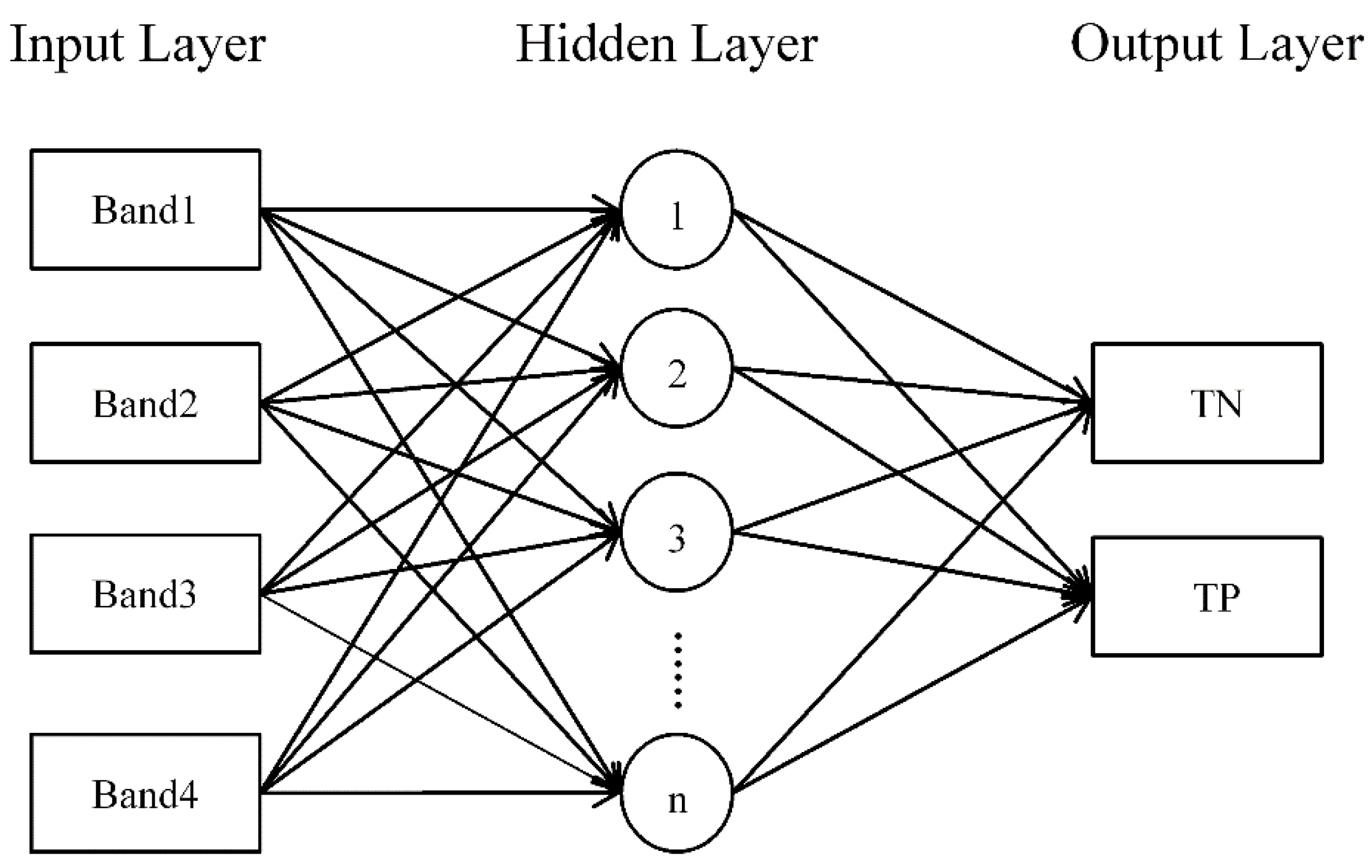According to the literature (Table 1), the methods could generally be divided into two categories: traditional linear regression model and intelligent algorithms. In recent studies, intelligent algorithms such as artificial neural network (ANN) [6,17,22,23] and support vector machine (SVM) models [21,24,25] have been increasingly used in this field. Therefore, a traditional multiple linear regression (MLR) model and an ANN model are chosen to estimate TN and TP concentrations of urban water bodies in China.

Few studies have found answers to the question of whether satellite imagery can successfully be applied to the remote sensing of water quality in urban water bodies of small area. Most studies focused on lakes and rivers with larger spatial scale. Among these studies, the imagery from Landsat/TM sensors was most commonly applied in the estimation of water quality parameters [15,19,22,26,27,28]. However, the 30 m spatial resolution of Landsat/TM imagery is not suitable for the narrow width and small area of urban water bodies, especially urban rivers. Therefore, higher resolution satellite is necessary to determine water quality of small urban water bodies. IKONOS imagery has four multispectral bands similar to Landsat/TM bands 1–4 and high (4 m) spatial resolution, making it a good candidate for applying previous methods to assess smaller lakes and ponds [29,30]. Currently, only a few studies have used the high spatial resolution satellite imagery such as IKONOS to monitor water quality. For example, Sawaya et al. [31] showed a strong relationship (R² = 0.89) between water clarity dataset and spectral-radiometric response of IKONOS data. Ekercin [32] used the IKONOS multispectral data to determine SD, Chl-a, and TSS in Gold Horn, Istanbul; the measured and estimated values of all three water quality parameters are in good agreement (R² > 0.97). Shamis [33] developed empirical models using linear regression analysis to retrieve Chl-a, TSS, and TP concentrations in the Sazlıdere reservoir, Turkey by IKONOS imagery, and produced a commonly good performance with R² ranging from 0.65 to 0.98. These studies show the potential application of IKONOS in the field of remote sensing of water quality; however, few studies have applied IKONOS imagery to directly determine TN and TP in small urban water bodies.

This study took Lake Cihu (Huangshi, China) and the lower reaches of Wen-Rui Tang river (Wenzhou, China) as examples to (1) evaluate the ability of IKONOS imagery data for determining TP and TN in urban water bodies, (2) estimate the TP and TN concentration in Lake Cihu and lower reaches of Wen-Rui Tang (WRT) River using regression and ANN models, (3) compare the performance between the models using in situ data, and (4) map TP and TN concentrations using the best model and IKONOS imagery data. The purpose of this paper is to present a cost-effective method to monitor TP and TN in urban water bodies while significantly reducing sampling time.

2. Study Area

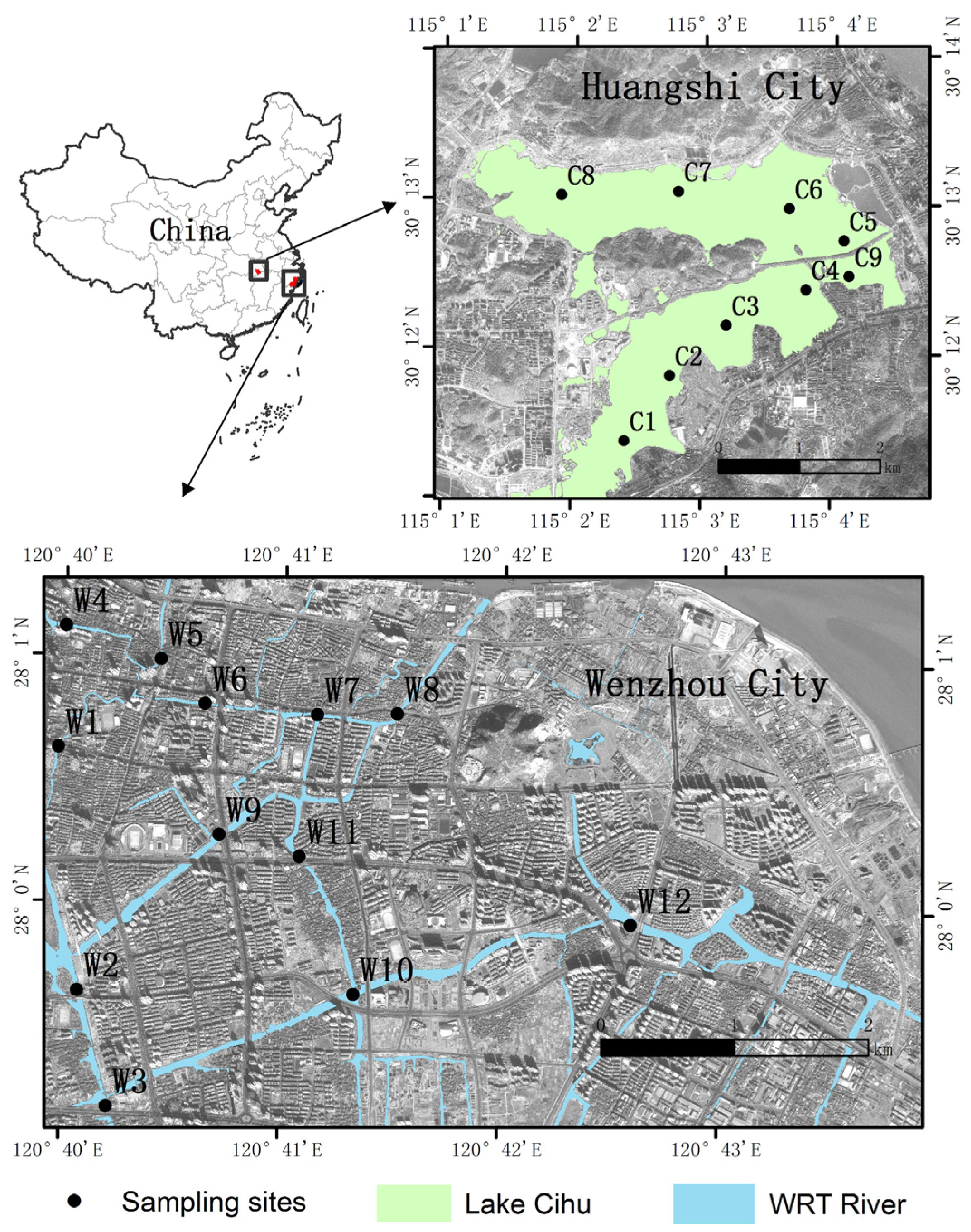
The selected areas for this study are Lake Cihu, an urban lake in Huangshi city, and the lower reaches of WRT River, an urban river that crosses Wenzhou city (Figure 1). These two urban water bodies represent two cities, which have different levels of urbanization and are separated by a long distance. These two urban water bodies are chosen to improve the universality of the methods used in this study. Lake Cihu is located in the northeast of Huangshi city along the southwestern bank of one of the major bends in the Yangtze River. It covers an area of approximately 9 km² from 30°10′46.71″ N to 30°13′22.50″ N in latitude, and 115°01′7.44″ E to 115°04′34.58″ E in longitude. It has a catchment area of 62.19 km², an average depth of 1.75 m, a shoreline of 38.5 km, and is connected to the Yangtze River by Shengyang sluice gate. The lower reaches of WRT River run through an urban district in Wenzhou City, a metropolitan area with a population of about seven million. This area has a catchment area of about 28 km² from 27°59′6″ N to 28°1′20″ N in latitude, and 120°39′56″ E to 120°43′50″ E in longitude. More than 75% of the watershed consists of a flat alluvial plain with elevations ranging from 3.0 to 4.2 m [4]. The average width of the urban portion of the WRT River is about 50 m, with a range from 8 to 150 m.

Figure 1. Location of study areas and sampling sites.

Figure 1. Location of study areas and sampling sites.

Considering their geographic features, the two urban water bodies play an important role in their respective cities. Lake Cihu is one part of Huangshi Riverside Business Central Axis. The WRT River is the “mother” river supporting the city for transportation, aquaculture, agriculture, drinking water, and other aspects of daily life. However, with the rapid industrial growth and urbanization in recent years, the cities have generated large volumes of untreated sewage and urban runoff pollution, which are discharged directly into the lake and river systems. The two urban water bodies do not currently meet the Type V national water quality standards [34], which is the lowest water quality standard that supports aquatic ecosystem health [35,36]. Therefore, effectively monitoring the TN and TP of the two urban water bodies has become a serious task.

3. Study Data

3.1. In Situ Data Collection

A total of nine temporary observatories in Lake Cihu are installed and operated from May 2011 to April 2012 (Figure 1). The locations of the sampling sites are selected by visually assessing water color differences shown in an IKONOS image acquired in May 2011. Water quality data of WRT river are obtained from the Wenzhou Municipal Planning Department. These data included six water quality parameters measured monthly at 12 water quality monitoring sites between November 2008 and October 2009. A YSI 6920 multi-parameter water quality sonde (YSI Inc., Yellow Springs, OH, USA) was attached to a boom from shore or a motor boat at 1 m depth and the location of each sampling point was determined with a Trimble GEO-XH2005 GPS (Trimble Navigation Limited, Sunnyvale, CA, USA). The YSI sonde was used to collect real-time water quality data: pH, water temperature, dissolved oxygen (DO), total ammonia nitrogen (NH₄⁺-N), and electrical conductivity (EC). Each water quality parameter was calibrated prior to data acquisition and the calibration was verified at the end of the sampling period (3 h). All water samples for direct TP and TN measurements are collected in 500 mL HDPE bottles and shipped back to laboratory in a cooler with ice packs. TP was analyzed using an ammonium molybdate spectrophotometric method after the samples are digested with potassium peroxydisulfate. TN was determined through a potassium persulfate oxidation-ultraviolet spectroscopy method. All the samples are analyzed in the laboratory within 48 h of water sampling. Sampling, preservation, transportation, and analysis of the water samples are implemented by following standard methods [37]. During the period of monitoring, the commercial satellite IKONOS had limited image across the study area. Therefore, only two IKONOS image data are used to correlate with the in situ TN and TP concentrations, one for Lake Cihu on 14 November 2011 and the other for the lower reaches of WRT River on 21 December 2008. Table 2 shows the in situ data obtained on 17 November 2011 in Lake Cihu (9 samples) and 20 December 2008 in the lower reaches of WRT river (12 samples), which are concurrent with IKONOS sensor overpass.

Table 2. TP and TN concentrations obtained from the different sampling sites identified in Figure 1.

Water Regions	Sampling Date	Data Subset	Sites	TN(mg/L)	TP(mg/L)
WRT River	20 December 2008	Calibration	W1	10.55	0.87
			W4	18.28	1.19
			W5	21.25	1.31
			W6	14.93	1.01
			W8	9.09	0.63
			W7	9.09	0.73
			W9	9.14	0.58
			W11	7.13	0.60
		Validation	W2	7.36	0.58
			W3	7.62	0.58
			W10	8.75	0.66
			W12	11.30	0.73
Lake Cihu	17 November 2011	Calibration	C1	1.80	0.13
			C2	1.53	0.13
			C3	1.54	0.13
			C4	1.62	0.13
			C5	1.22	0.07
			C6	1.05	0.08
		Validation	C7	0.96	0.08
			C8	1.03	0.10
			C9	1.30	0.10

Table 2. TP and TN concentrations obtained from the different sampling sites identified in Figure 1.

Water Regions	Sampling Date	Data Subset	Sites	TN(mg/L)	TP(mg/L)
WRT River	20 December 2008	Calibration	W1	10.55	0.87
			W4	18.28	1.19
			W5	21.25	1.31
			W6	14.93	1.01
			W8	9.09	0.63
			W7	9.09	0.73
			W9	9.14	0.58
			W11	7.13	0.60
		Validation	W2	7.36	0.58
			W3	7.62	0.58
			W10	8.75	0.66
			W12	11.30	0.73
Lake Cihu	17 November 2011	Calibration	C1	1.80	0.13
			C2	1.53	0.13
			C3	1.54	0.13
			C4	1.62	0.13
			C5	1.22	0.07
			C6	1.05	0.08
		Validation	C7	0.96	0.08
			C8	1.03	0.10
			C9	1.30	0.10

3.2. Satellite Image Processing

IKONOS was launched on 24 September 1999 from Space Launch Complex 6, Lompoc, CA, USA, and was the first to collect publicly available high-resolution imagery at four-meter spatial resolution. The spectral characteristics of the satellite sensor are given in Table 3. According to the principle of low cloud cover, two images acquired on 21 December 2008 for the lower reaches of WRT River and on 14 November 2011 for Lake Cihu are selected for analysis. The images are ordered from IntraSearch, Inc. (Lone Tree, CO, USA), an authorized United States Geological Survey (USGS) business partner and distributor of other commercial digital and hard copy datasets. The satellite imagery acquired and ground observations are collected at varying times, differing by one and three days, respectively. Some studies have concluded that measurements taken within a few days (±3 days to 10 days) of image acquisition provide strong relationships, e.g. reference [38]. However, other studies have shown that there can be weak correlation between satellite images and in situ measurements when taken on different dates, e.g. reference [39]. In this study, the meteorological data (rainfall, temperature and wind speed) provided by the Shared Services Network of the China Meteorological Administration during these one- and three-day gaps in Huangshi and Wenzhou, respectively, have been collected. In Table 4, it can be seen that the wind speed are lower than 1.5 m/s, the rainfall are lower than 0.1 mm and the temperature changed little during these one- and three-day gaps. Therefore, it is considered that the weather conditions did not influence the state of water condition and, therefore, the concentrations of TN and TP did not change during these one- and three-day gaps.

Table 3. Comparison of spectral characteristics of the four IKONOS bands used in this study and the first four Landsat/TM bands.

Satellite	Band	Spectral Region (μm)	Bandwidth (μm)	Centre Wavelength (μm)
IKONOS	1	0.45–0.52	0.07	0.48
	2	0.51–0.60	0.09	0.55
	3	0.63–0.70	0.07	0.66
	4	0.76–0.85	0.09	0.81
Landsat/TM	1	0.45–0.52	0.07	0.49
	2	0.52–0.60	0.08	0.56
	3	0.63–0.69	0.06	0.66
	4	0.76–0.90	0.14	0.83

Table 3. Comparison of spectral characteristics of the four IKONOS bands used in this study and the first four Landsat/TM bands.

Satellite	Band	Spectral Region (μm)	Bandwidth (μm)	Centre Wavelength (μm)
IKONOS	1	0.45–0.52	0.07	0.48
	2	0.51–0.60	0.09	0.55
	3	0.63–0.70	0.07	0.66
	4	0.76–0.85	0.09	0.81
Landsat/TM	1	0.45–0.52	0.07	0.49
	2	0.52–0.60	0.08	0.56
	3	0.63–0.69	0.06	0.66
	4	0.76–0.90	0.14	0.83

Table 4. Observed meteorological data during date gap.

Meteorological Station	Date	Wind Speed	Rainfall	Average Temperature	Maximum Temperature	Minimum Temperature
Huangshi	14 November 2011	0.6	0	15.7	21.0	11.3
	15 November 2011	0.7	0	15.3	21.6	11.0
	16 November 2011	1.5	0	16.4	22.6	12.2
	17 November 2011	1.1	0	18.9	25.2	13.9
Wenzhou	20 December 2008	0.6	0	14.6	22.7	9.1
	21 December 2008	1.1	0.1	13.5	22.5	10.2

Table 4. Observed meteorological data during date gap.

Meteorological Station	Date	Wind Speed	Rainfall	Average Temperature	Maximum Temperature	Minimum Temperature
Huangshi	14 November 2011	0.6	0	15.7	21.0	11.3
	15 November 2011	0.7	0	15.3	21.6	11.0
	16 November 2011	1.5	0	16.4	22.6	12.2
	17 November 2011	1.1	0	18.9	25.2	13.9
Wenzhou	20 December 2008	0.6	0	14.6	22.7	9.1
	21 December 2008	1.1	0.1	13.5	22.5	10.2

To directly obtain TN and TP concentrations from the reflectance of the satellite images, all four IKONOS bands from visible and NIR ranges of each image are processed for radiometric calibration, atmospheric correction, and geometric correction, as described elsewhere [40,41]. Radiometric calibration is used to convert the digital number (DN) recorded by the sensor to spectral radiance and to minimize errors caused by the sensor by using the following equation:

$$L_i=\frac{D{N}_i\times {10}^4}{CalCoe{f}_i\times Bandwidt{h}_i}$$

(1)

where L_i is radiance for spectral band i at the sensor’s aperture; DN_i is the digital number for spectral band i; CalCoef_i is the radiometric calibration coefficient; and Bandwidth_i is the bandwidth of spectral band i. Since the IKONOS image used in this study was acquired after 22 February 2001, the values of the calibration coefficients for the 11-bit IKONOS products are 728 for band 1727 for band 2949 for band 3, and 843 for band 4 [42]. The bandwidths for IKONOS bands are obtained from the IKONOS product manual.

Atmospheric correction was performed using the fast line-of-sight atmospheric analysis of spectral hypercube (FLAASH) module in ENVI 5.0 (Exelis Visual Information Solutions, Inc. Boulder, USA). FLAASH is a first-principle atmospheric correction tool that corrects wavelengths in the visible through near-infrared and shortwave infrared regions up to 3 μm. It incorporates the MODTRAN 4 radiation transfer code. FLAASH is widely used to eliminate the effects of the atmosphere, and convert spectral radiance to surface reflectance of water. Geometric accuracy of the multispectral imagery is checked by ground control points.

To improve image quality by removing errors resulting from GPS (Global Positioning System) measurements in the fieldwork and eliminate noise, mean spectra of 3 × 3, 5 × 5, 7 × 7, 9 × 9, and 11 × 11 windows centered at the sampled locations in Lake Cihu are tested by low-pass filtering. Figure 2 shows the changing pattern of average surface reflectance values of all nine samples with increasing kernel size. The average surface reflectance value becomes relatively stable when the kernel size is 5 × 5. However, low-pass filtering is not suitable for the lower reaches of WRT River because its extremely narrow width will cause some of the windows to include land pixels. Therefore, five water pixels close to the sample pixel are chosen instead of the window, and their average surface reflectance values are used to correlate measured TN and TP concentrations with the IKONOS multispectral imagery.

Figure 2. Average surface reflectance of nine samples in Lake Cihu with different pixel array sizes.

Figure 2. Average surface reflectance of nine samples in Lake Cihu with different pixel array sizes.

4. Methodology

4.1. Multiple Linear Regression

MLR uses linear statistics to model the relationship between a scalar dependent variable and several independent explanatory variables. Several multiple regressions are used to explore the relationships between water quality parameters and IKONOS data in the study area. This model assumes the following form:

$$WQPs=A_0+{\displaystyle \sum _{i=1}^k\left(A_i\times IKONO{S}_i\right)}$$

(2)

where WQPs is the water quality parameter concentrations; IKONOS_i is the surface reflectance of the four IKONOS bands and their combinations; k is the IKONOS band and band combination number; and A₀ and A_i are the empirical regression coefficients derived using the observations from the in situ data [32]. Based on previous studies of the relationships between spectral characteristics with WQPs, 4 bands and their combinations were selected for statistical analysis in this study. These combinations fell into two categories. One category was the addition or subtraction combination of any two bands, e.g., Band 1 + Band 2, the other was the ratio combination of any two combinations in first category, e.g., (Band 1 + Band 2)/(Band 1 − Band 2). A significance level p = 0.05 is used to denote statistically significant relationships between in situ WPQs concentrations and surface reflectance of bands or their combinations. Statistical software SPSS 18.0 (IBM SPSS, Inc. New York, NY, USA) is used for the regression and statistical analysis.

4.2. Artificial Neural Network

A network with a hyperbolic tangent function hidden layer and a linear output layer is proven capable of characterizing any static nonlinear relationship [43]. Therefore, an ANN with three layers, consisting of an input layer, a hyperbolic tangent function hidden layer, and a linear output layer, is established using MATLAB 2011a (MathWorks, Inc. Natick, MA, USA) (Figure 3). The input data includes water surface reflectance of the four IKONOS bands and their corresponding WQPs concentration values were the output data. All input IKONOS band data were preprocessed, and TN and TP concentrations were scaled to [0,1] by a factor depending on the valid range of parameters, i.e., the difference between maximum and minimum values of each water quality parameter is considered.

For the hidden layer, no theoretical background is found to indicate how many neurons should be selected; hence, concrete conditions must be analyzed by trial and error. If the neurons are too few, the self-learning ability and precision of network will decrease. Meanwhile, if too many neurons are selected, training time will increase and the generalization ability of the network will decrease [44,45]. Therefore, a balance between the two scenarios must be obtained. By comparing the results of ANN models with different hidden layer neurons from 3 to 15 empirically, an ANN with 10 hidden layer neurons is selected.

Figure 3. A neural network diagram for this study.

Figure 3. A neural network diagram for this study.

The weights assigned to each connection were randomly generated before training the model and were estimated based on the back-propagation algorithm. The minimum error for each trial is calculated using the Leverberg-Marquardt method. The algorithm stops when RMSE is not greater than a cutoff value. The cutoff value is chosen empirically, based on the results of analysis using several cutoff values, starting from 0.5 mg/L and decreasing until an acceptable output is achieved. The weight configuration returning the smallest error is applied to the ANN model.

5. Results

5.1. Regression Analysis

The Pearson’s correlation coefficient between the four IKONOS bands and the two water quality parameters in 21 samples are shown in Table 5. TN and TP concentrations have a strong negative correlation with all four IKONOS bands. The correlations of all visible and near-infrared bands with TN concentrations are higher than −0.7, and the highest correlation of Band 2 (green region) is −0.93. The same is true for TP: the highest correlation of Band 3 (red region) is −0.93, and the lowest correlation of Band 1 (blue region) is −0.77.

Table 5. Pearson’s correlation coefficient among TN and TP with IKONOS bands and band combinations.

WQP	B1	B2	B3	B4	B1/B4	B2/B4	B3/B4	B1/B3	B2/B3
TN	−0.81 **	−0.93 **	−0.92 **	−0.89 **	0.75 **	0.65 **	0.47 *	0.88 **	0.82 **
TP	−0.77 **	−0.91 **	−0.93 **	−0.91 **	0.80 **	0.71 **	0.54 *	0.90 **	0.85 **
WQP	B1/B2	$\frac{B4-B1}{\mathit{B}\mathbf{4}-\mathit{B}\mathbf{2}}$	$\frac{B2-B1}{\mathit{B}\mathbf{4}-\mathit{B}\mathbf{2}}$	B1+B2	$\frac{B3-B1}{\mathit{B}4-\mathit{B}3}$	$\frac{B4-B1}{\mathit{B}4-\mathit{B}3}$	$\frac{B3-B1}{\mathit{B}4-\mathit{B}2}$	$\frac{B1}{\mathit{B}1+\mathit{B}2}$	$\frac{B2}{\mathit{B}1+\mathit{B}2}$
TN	0.89 **	0.89 **	0.88 **	−0.90 **	0.89 **	0.88 **	0.87 **	0.87 **	0.88 **
TP	0.91 **	0.90 **	0.91 **	−0.88 **	0.91 **	0.89 **	0.89 **	0.89 **	0.89 **

Notes: **, p-value less than 0.01; *, p-value less than 0.05.

Table 5. Pearson’s correlation coefficient among TN and TP with IKONOS bands and band combinations.

WQP	B1	B2	B3	B4	B1/B4	B2/B4	B3/B4	B1/B3	B2/B3
TN	−0.81 **	−0.93 **	−0.92 **	−0.89 **	0.75 **	0.65 **	0.47 *	0.88 **	0.82 **
TP	−0.77 **	−0.91 **	−0.93 **	−0.91 **	0.80 **	0.71 **	0.54 *	0.90 **	0.85 **
WQP	B1/B2	$\frac{B4-B1}{\mathit{B}\mathbf{4}-\mathit{B}\mathbf{2}}$	$\frac{B2-B1}{\mathit{B}\mathbf{4}-\mathit{B}\mathbf{2}}$	B1+B2	$\frac{B3-B1}{\mathit{B}4-\mathit{B}3}$	$\frac{B4-B1}{\mathit{B}4-\mathit{B}3}$	$\frac{B3-B1}{\mathit{B}4-\mathit{B}2}$	$\frac{B1}{\mathit{B}1+\mathit{B}2}$	$\frac{B2}{\mathit{B}1+\mathit{B}2}$
TN	0.89 **	0.89 **	0.88 **	−0.90 **	0.89 **	0.88 **	0.87 **	0.87 **	0.88 **
TP	0.91 **	0.90 **	0.91 **	−0.88 **	0.91 **	0.89 **	0.89 **	0.89 **	0.89 **

Notes: **, p-value less than 0.01; *, p-value less than 0.05.

Correlation analysis is also undertaken with IKONOS band ratios. Table 5 shows that the correlation between TN or TP concentrations and any band ratio are not higher than that for single band. This result is in accordance with the research of Song et al. [17], but different from several other studies [15,19]. Band ratios can reduce some random noise caused by illumination and background; however, they do not necessarily improve empirical models with imagery data [17,46]. All other band combinations mentioned above were analyzed although most did not show superiority to the single bands (seen in Table 5). A stepwise linear regression model is established with the four IKONOS bands and all band ratios and combinations. A data subset of 14 samples (six from Lake Cihu and eight from the lower reaches of WRT River) is used to establish the regression models. By comparing all the multiple regression models, in consideration of the coefficient of determination, residual analysis, and 95% confidence intervals, the best model is selected to evaluate TN and TP concentrations, as follows:

$$TN=-276.02\times Band2+54.56$$

(3)

$$TP=-15.51\times Band3+2.81$$

(4)

where TN and TP are the TN and TP concentrations (mg/L), and Band2 and Band3 are the surface reflectance of IKONOS Band 2 and Band 3. The model equations show that the band ratio algorithms do not always improve water parameter inversion accuracy, and single IKONOS bands often have higher correlation with water quality variables in this study. The remaining part of the dataset is used to validate these empirical models. Finally, coefficients of determination (R²) and root mean square error (RMSE) were calculated with all samples. The model calibration and validation results are shown in Table 6 and Figure 4. Application of MLR models to determine TN and TP yielded R² values of 0.85 and 0.84, respectively, for the calibration samples, and 0.88 and 0.87, respectively, for validation samples. Furthermore, residual analysis is conducted to test the model outputs. Figure 5a,c show that the standardized residual of each sample in calibration dataset for both TN and TP models is in [–2,2], and Figure 5b,d show the normal P-P plot of regression standardized residual of the two models. The residual analysis results verified that these two models were acceptable and valid. The calibration and validation results also show that the regression models demonstrate good performance for both TN and TP.

Table 6. Comparison of inversion accuracy of MLR middle and ANN model.

WQP	MLR							ANN
	95% Confidence Interval			Calibration		Validation		Calibration		Validation
	Term	Lower Bound	Upper bound	R2	RMSE (mg/L)	R2	RMSE (mg/L)	R2	RMSE (mg/L)	R2	RMSE (mg/L)
TN	Constant	42.25	66.86	0.85	2.50	0.88	1.47	0.99	0.63	0.96	0.89
	Band2	−347.94	−204.09
TP	Constant	2.196	3.431	0.84	0.17	0.87	0.09	0.98	0.06	0.85	0.14
	Band3	−19.669	−11.356

Table 6. Comparison of inversion accuracy of MLR middle and ANN model.

WQP	MLR							ANN
	95% Confidence Interval			Calibration		Validation		Calibration		Validation
	Term	Lower Bound	Upper bound	R2	RMSE (mg/L)	R2	RMSE (mg/L)	R2	RMSE (mg/L)	R2	RMSE (mg/L)
TN	Constant	42.25	66.86	0.85	2.50	0.88	1.47	0.99	0.63	0.96	0.89
	Band2	−347.94	−204.09
TP	Constant	2.196	3.431	0.84	0.17	0.87	0.09	0.98	0.06	0.85	0.14
	Band3	−19.669	−11.356

Figure 4. Relationship between measured and predicted TN (a,b) and TP (c,d) concentrations with both MLR and ANN models using IKONOS images.

Figure 4. Relationship between measured and predicted TN (a,b) and TP (c,d) concentrations with both MLR and ANN models using IKONOS images.

Figure 5. Standardized residual plot (a,c) and Normal P-P plot of regression standardized residual (b,d) of MLR models.

Figure 5. Standardized residual plot (a,c) and Normal P-P plot of regression standardized residual (b,d) of MLR models.

5.2. Artificial Neural Network

Similarly, all the sample data sets (n = 21) were divided into two groups. One group (n = 14) is used to train the ANN, and the rest (n = 7) is used to test the ANN model. The output of the network is compared to the in situ measurements of TN and TP concentrations. The algorithm stops when RMSE is not greater than a given cutoff value. By analyzing the performance of the ANN models with different cutoff values, the value 0.23 mg/L is accepted. The algorithm stops after 31 iterations, and the RMSE values are 0.63 and 0.06 mg/L for TN and TP, respectively. Validation of the neural network is done with the other group of data subset (n = 7). RMSE and R² of the simulation results are calculated with all samples (see Table 6). The ANN model demonstrates good performance for both calibration and validation samples, in which R² values range from 0.85 to 0.99. Correspondingly, the RMSE values range from 0.06 to 0.89 mg/L.

5.3. Retrieval Accuracy Comparison

The mean value and variance of measured and estimated concentration of TN and TP are close, as shown in Table 7. Based on R² and RMSE values (Table 6), the estimation accuracy greatly improves when the ANN model is applied. The relative RMSE (RMSE over measured average water quality parameters) of the estimation resulting from using the ANN model are 10.4% for TN and 13.4% for TP. These values are significantly lower than the relative RMSE values resulting from the regression analysis, with the corresponding values of 31.6% for TN and 29.4% for TP. A graphical comparison between the results for the MLR and ANN models for TN and TP is shown in Figure 4. By comparing the estimated and measured TN concentration, Figure 4a,b shows that the results derived from the ANN model for both calibration and validation dataset are very closely distributed along the 1:1 line, while several samples far from the 1:1 line are found in the results derived from the MLR model. Figure 4c,d shows the performance of estimated TP concentration derived from the two models. Even if two validation samples stray from the 1:1 line in the ANN model results, its performance is superior to MLR in general. Figure 4 is not satisfying for MLR because only one band is used. A better method would be to plot observed and predicted vs. the band value. The relationship between the surface reflectance of the selected band and measured and predicted data with MLR models are shown in Figure 6.

Table 7. Summary statistics of measured WQPs and estimated WQPs by two models.

WQP	Data Subset	Measured Data		MLR		ANN
		Mean (mg/L)	Variance	Mean (mg/L)	Variance	Mean (mg/L)	Variance
TN	Calibration	7.73	45.86	7.76	38.58	7.71	43.84
	Validation	5.47	18.40	5.54	21.54	5.80	20.61
TP	Calibration	0.54	0.19	0.54	0.16	0.54	0.19
	Validation	0.40	0.09	0.41	0.08	0.43	0.14

Table 7. Summary statistics of measured WQPs and estimated WQPs by two models.

WQP	Data Subset	Measured Data		MLR		ANN
		Mean (mg/L)	Variance	Mean (mg/L)	Variance	Mean (mg/L)	Variance
TN	Calibration	7.73	45.86	7.76	38.58	7.71	43.84
	Validation	5.47	18.40	5.54	21.54	5.80	20.61
TP	Calibration	0.54	0.19	0.54	0.16	0.54	0.19
	Validation	0.40	0.09	0.41	0.08	0.43	0.14

Figure 6. Relationship between surface reflectance of band and measured data predicted (a) TN and (b) TP concentrations with MLR models.

Figure 6. Relationship between surface reflectance of band and measured data predicted (a) TN and (b) TP concentrations with MLR models.

5.4. Spatial Distribution of Water Quality Parameters

The ANN model is then applied to the IKONOS imagery data to estimate the value of both TN and TP concentrations at all locations in Lake Cihu and the lower reaches of WRT River. IKONOS image data is output as ASCII from ENVI to the ANN model for mapping these two water quality parameters. The resulting WQPs are then classified into groups and are used to depict spatial patterns in TN and TP across Lake Cihu (Figure 7) and the lower reaches of WRT River (Figure 8).

Figure 7. Spatial distribution maps of (a) TN and (b) TP over Lake Cihu.

Figure 7. Spatial distribution maps of (a) TN and (b) TP over Lake Cihu.

Figure 8. Spatial distribution maps of (a) TN and (b) TP over lower reaches of WRT River.

Figure 8. Spatial distribution maps of (a) TN and (b) TP over lower reaches of WRT River.

Figure 7a shows the predicted TN concentration distribution in Lake Cihu on 14 November 2011, with an average value of 1.63 mg/L and a standard deviation of 0.56 mg/L. The highest TN concentration is observed in the middle of the north of Lake Cihu, ranging from 1.3 to 2.4 mg/L. The predicted TN concentration is lower in the south of Lake Cihu where the value ranges between 0.5 and 1.8 mg/L. Spatial patterns of TP predicted from remote sensing in Lake Cihu are shown in Figure 7b. The predicted TP concentration has an average value of 0.18 mg/L and standard deviation of 0.12 mg/L. The distribution of TP concentration is similar to TN. The TP concentration in the north of Lake Cihu is much higher than in the south of Lake Cihu, especially near the lakeshore.

The distribution of predicted TN and TP concentrations along the lower reaches of WRT River on 21 December 2008 is shown in Figure 8a,b, respectively. The spatial patterns of predicted TN and TP concentrations are similar in the lower reaches of WRT River, as observed in Lake Cihu. This phenomenon states that TN/TP ratios of the whole water area are similar, and the measured data obtained during the one-year monitoring period support this finding. The reason for this finding could be that both TP and TN are from the same source (e.g., domestic wastewater). The predicted TN concentration has an average value of 8.98 mg/L and standard deviation of 7.34 mg/L. The predicted TP concentration has an average value of 0.72 mg/L and a standard deviation of 0.5 mg/L. The main stream of WRT River (left side of the image) from the rural zone has relatively low levels of TN and TP concentrations, ranging from 2 to 8 mg/L and from 0.1 to 0.5 mg/L, respectively. High TN and TP concentrations are observed in the tributary across the urban zone. The highest values, from 18 to 22 mg/L of TN and 1.2 to 2.0 mg/L of TP, are present in an artificial lake in Yangfushan Park on the northeast portion of the WRT River.

6. Discussion

The aim of this study is to retrieve TN and TP concentrations of relatively small urban water bodies by satellite images. Previous studies mainly focused on large spatial scale water bodies, such as Lake Taihu (2338 km²), Lake Chaohu (789 km²), and Qiantang River (about 150–500 m wide). As a result, the moderate-resolution imaging spectroradiometer (MODIS) with 250 m spatial resolution and Landsat/TM with 30 m spatial resolution have been widely applied to determine TN and TP concentrations [14,15,16,19,21,47]. However, the low spatial resolution remote sensing images provided by the abovementioned satellite sensors are not applicable to small-scale urban water bodies, especially urban rivers several meters wide. To solve this problem, high spatial resolutions IKONOS multispectral imagery, which has four multispectral bands similar to Landsat/TM bands 1–4 and 4 m spatial resolution, is used in this study. The statistical analysis reveals that both MLR and ANN models have highly accurate inversion results for TN and TP concentrations. This good performance demonstrates that the IKONOS satellite data has adequate potential to determine TN and TP concentrations in urban water bodies at a relatively small scale.

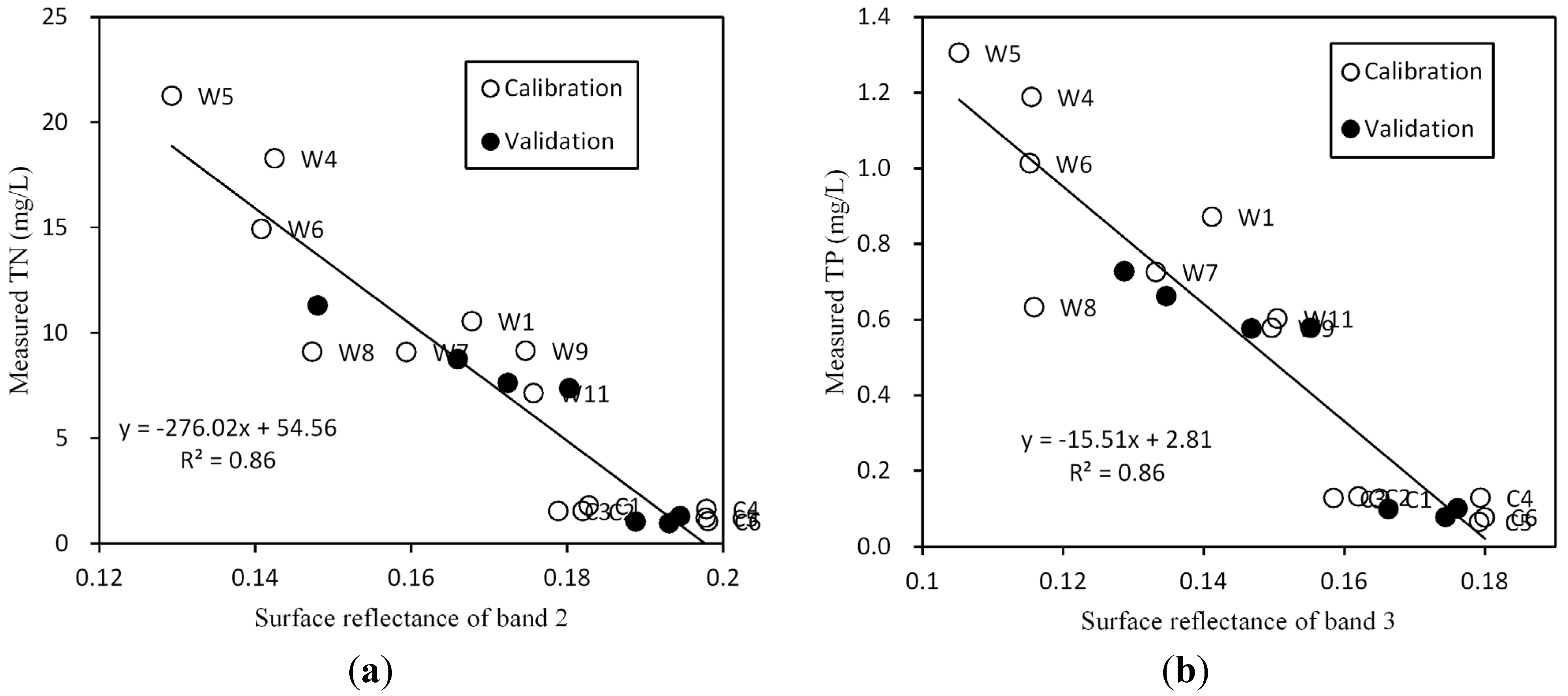
Another advancement made in this study is to establish two inversion equations to retrieve both TN and TP from urban water bodies. Compared to the existing TN and TP inversion equations shown in Table 1, these two equations (Equations (3) and (4)) have relatively simple forms and only require a single band instead of band ratios in the right-hand side because of high correlations between IKONOS bands and in situ TN and TP data. Three possible reasons for this condition are considered, as follows:

(1)

The commercial satellite has limited image archives across the study area because of the lack of research using the IKONOS images in the area. As a result, little IKONOS image data are available to correlate with the in situ TN and TP concentrations.

(2)

The spatial detail of high-resolution IKONOS images is impressive. However, the problem of spectral-radiometric similarity between certain classes is compounded. Mixed pixels are still present, and the variability within classes may be greater than in lower-resolution images [29]. The resulting high-interclass and low-interclass variability may lead to a reduction in the statistical separability of the different classes in the spectral domain. This characteristic of IKONOS images may be one factor that differentiates it from the images of middle and low spatial resolution satellites, such as MODIS and Landsat/TM. To overcome this inadequacy and complement the spectral feature space, textural, structural, scale, and object-based features should be effectively exploited in future studies.

(3)

Several studies [48,49,50,51] revealed that lake or river water quality is highly dependent on the landscape characteristics with respect to watershed and geographical scales. Therefore, the difference in water quality configurations between urban water in this study and the large lakes and rivers examined in previous studies may lead to the differences in the relationships of surface reflectance and TN and TP concentrations.

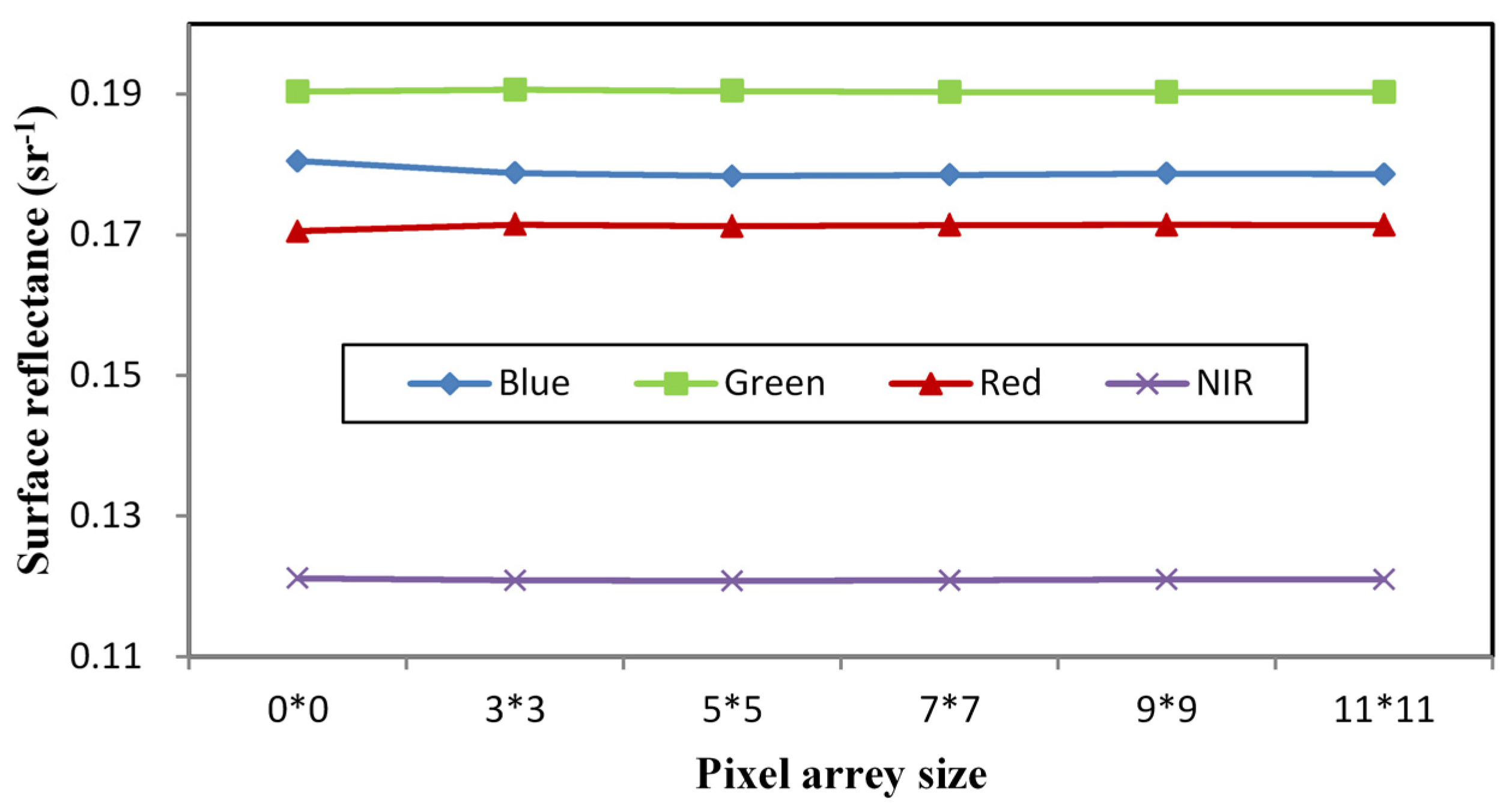
For optically shallow water, water quality parameters can be usually interferential because of the bottom disturbance [52,53]. Lake Cihu is shallow with water depth ranging from 0.72 to 5.73 m; however, water with average turbidity of more than 34 NTU (Nephelometric Turbidity Unit) is too turbid to see the bottom, even when water is near the shore. It can be considered as optically deep water. The contribution from the bottom of optically deep water has little effect to the intensity and spectral distribution of remotely sensed signal above the water surface [52,54]. Therefore, the potential backscattering issues from the lake bottom were not considered in this study. However, in some very shallow locations, the potential backscattering issues from the lake bottom may bring some errors, and the estimated TN and TP concentrations may not be very reliable. Under these circumstances, incorporating additional information on water depth, such as bathymetric data, would be better in the modeling activities to avoid any misinterpretation of the results.

Like in many other studies [6,15,17,21], all water samples and the two images collected are considered as the dataset. About 70% of the water samples, which are six samples from one water body and eight samples from the other water body, have been chosen to calibrate the models. The other seven water samples were used to validate the models. The approach of selecting data subsets used in this study can improve the performance of models, but may reduce the generalization ability of the models. In future studies, a variety of strategies for selecting data may be considered to calibrate and validate the models. For example, one image and its corresponding measured data can be used to calibrate models, and the other image and data are used for validation. Furthermore, some cross-validation methods like random forests (RF) can be considered.

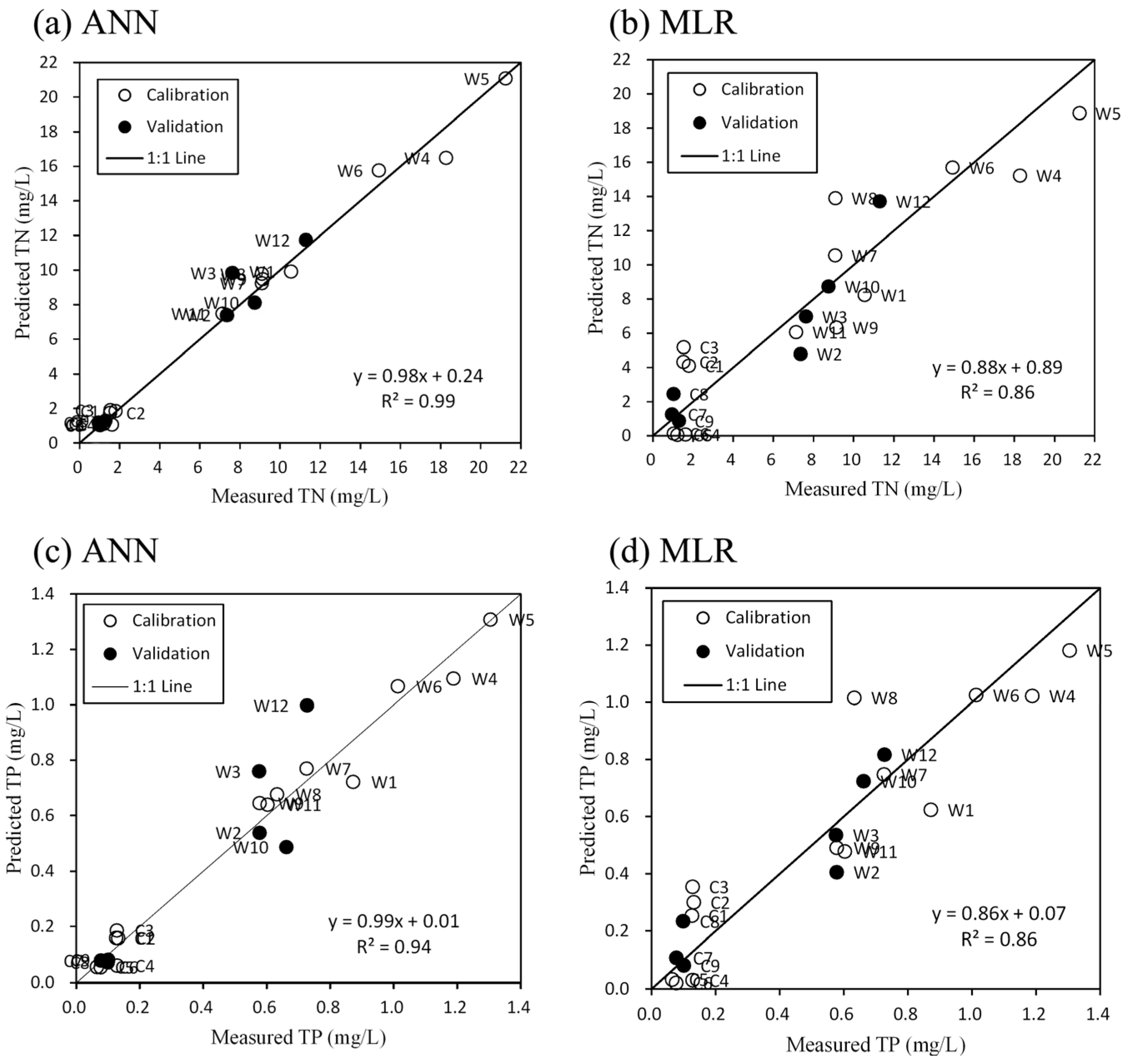
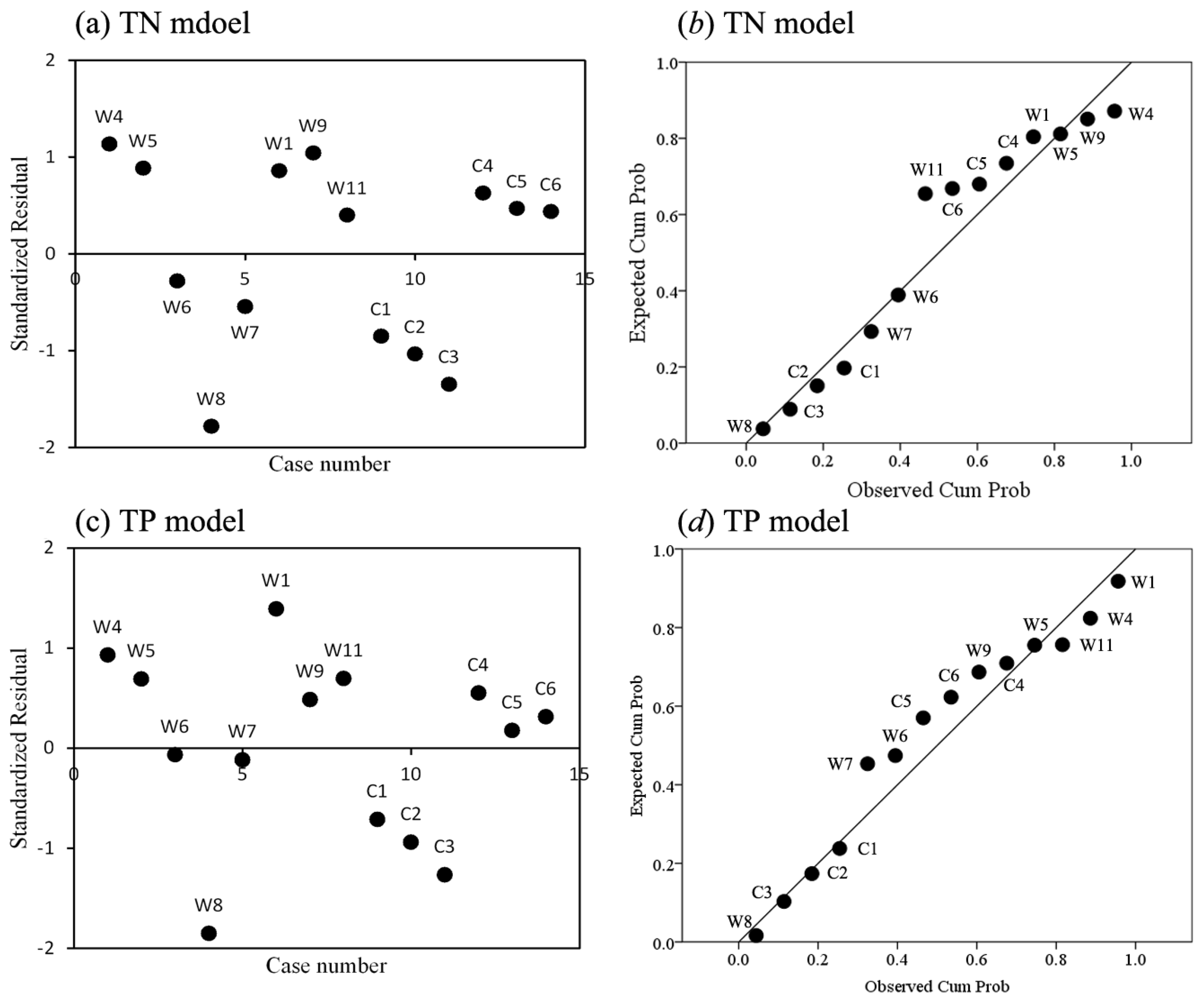
The statistical analysis of R² and RMSE, achieved by both linear (MLR) and nonlinear (ANN) models, supports the hypothesis that the relationships between reflectance and water quality parameters concentration are nonlinear, which is consistent with the conclusions in previous studies [6,17,32,41,55]. Though the results demonstrate that the ANN model has a stronger ability to simulate the complex nonlinear relationship, it may be more prone to the effects of the local optimal solution developed on the basis of the empirical risk minimization theory [56]. In this study, two processing methods, i.e., data normalization and setting different hidden layer neurons, are applied in training the ANN model to overcome the network overfitting problem. However, the estimation accuracy for the TP validation data subset is still lower than the linear regression analysis. This unfavorable situation may be improved by new studies using other advanced intelligent methods, such as SVM and GA-PLS to obtain better-fitting results.

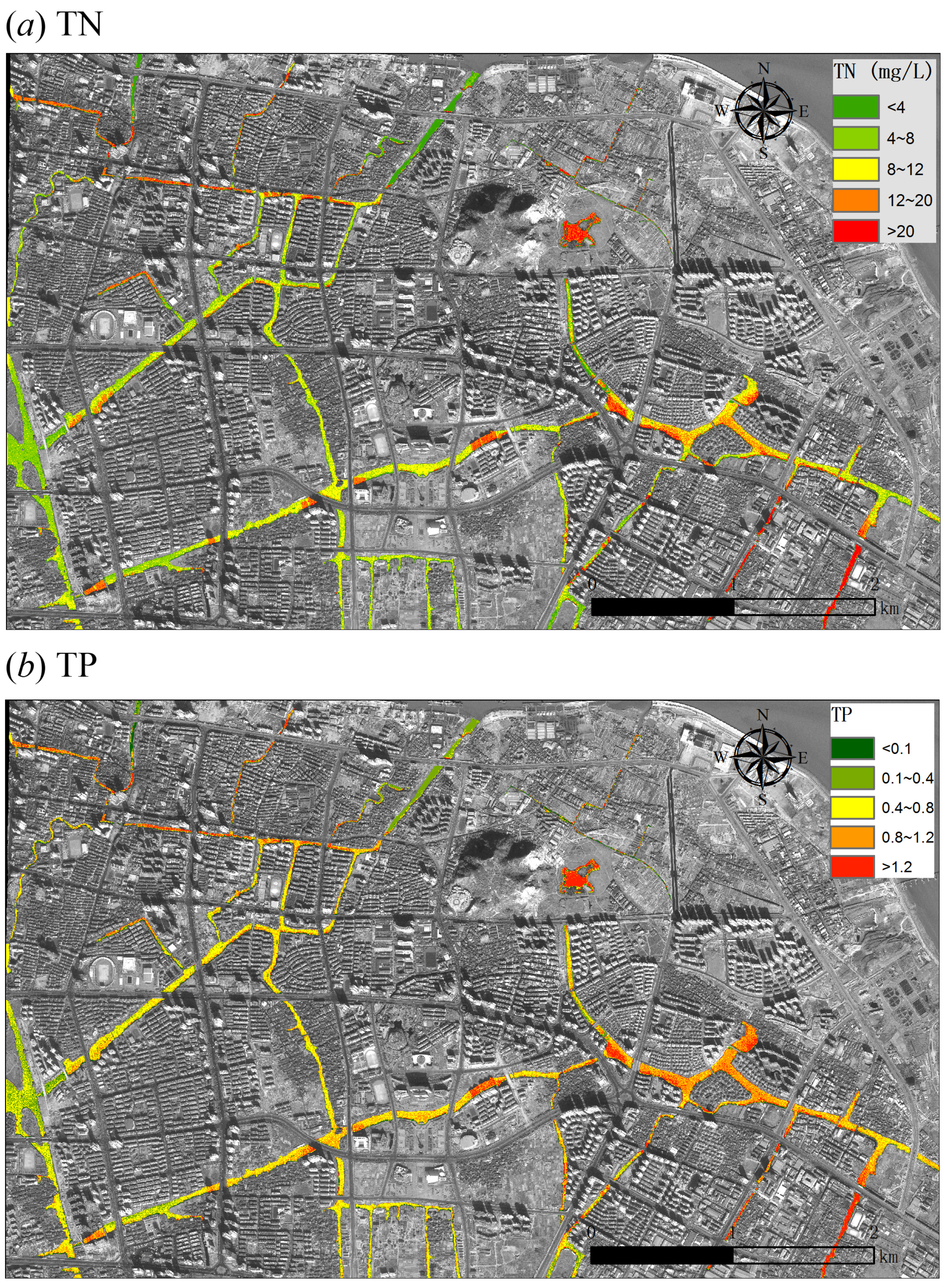
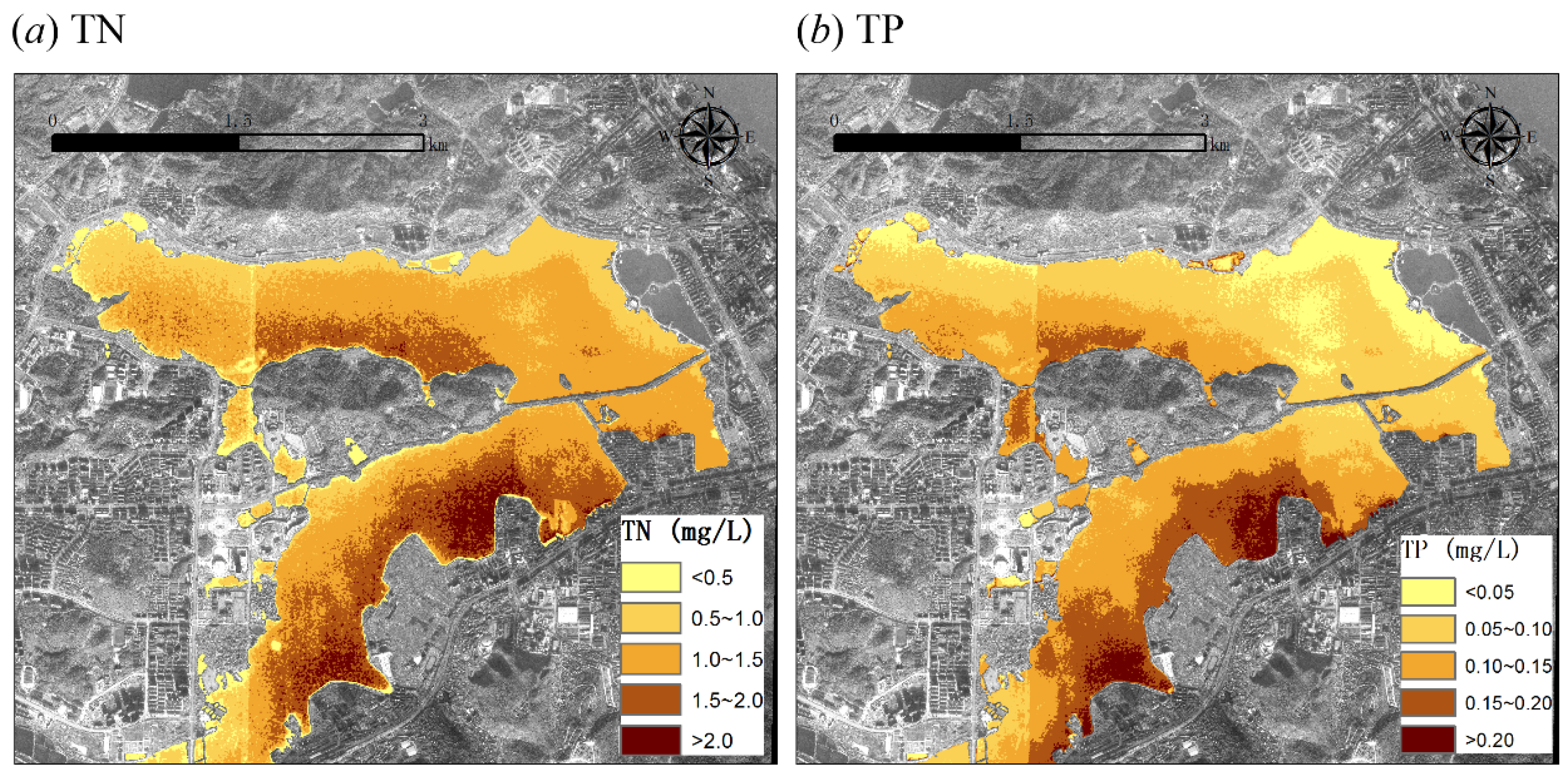
In Figure 5 and Figure 6, TP and TN concentration maps show that water quality near the residential and industrial areas is worse, most likely because of pollutants from domestic sewage and industrial wastewater. The Cihu map and previous reports [35,57] show many intensive residential quarters and several sewage plant outlets in the south of Lake Cihu, which contribute to high concentrations in the southern part of the lake. The main urban areas with highly-intensive residential area, where the WRT River flows through, can be seen clearly in the satellite image. TP and TN concentrations in the main stream from the rural zone are lower than that in tributary across the residential area. These observations are consistent with the results of previous studies [36,58].

This study reveals that degraded water quality is related to both anthropogenic activities and poor wastewater management. The two cities examined in this study have different levels of urbanization. Wenzhou, where WRT River flows through, is highly urbanized and is one of China’s most developed areas. By contrast, Huangshi (where Lake Cihu lies) is located in the middle of China and urbanization is currently relatively low. However, Huangshi’s urbanization course has greatly accelerated during recent years. Both Lake Cihu and the lower reaches of WRT River have become the main receivers of wastewater from their respective cities because of the lack of sanitation and uneven distribution of water treatment facilities during the urbanization process. These two urban water bodies indicate that the trends of TN and TP concentrations are very consistent in all of the water areas shown in Figure 8. By analyzing all in situ and water pixels data, we determine that TN and TP concentrations of the lower reaches of WRT River are about 8 to 12 times higher than those of Lake Cihu, thereby reflecting the effects of higher level of urbanization. However, a potential relationship has been found, in which the TN/TP ratios of Lake Cihu and the lower reaches of WRT River are very close. Therefore, the chemical compositions of these two urban water bodies are expected to be similar, which could lead to similar spectral distribution of remotely-sensed signal above water surface. If the chemical compositions of urban water polluted by industrial wastewater and domestic sewages are similar in cities with different levels of urbanization throughout China, future studies should examine this phenomenon in places where urban water quality data are available.

7. Conclusions

In this paper, the determination of TN and TP concentrations of small-sized urban water bodies from high-resolution IKONOS multispectral imagery are developed in two case studies. Both linear (MLR) and nonlinear (ANN) models are used to establish the relationship between water surface reflectance and TN and TP concentrations collected in the temporary observatories. The accuracies of these two models in this study are similar to those achieved in other similar studies (Table 1), supporting the applicability and validity of the models. The ANN model results give significantly consistent information with very high coefficients of determinations (R² = 0.98 and 0.94 for TN and TP, respectively). The MLR models have relatively simple forms and only require a single band to calculate TN and TP concentrations.

The water quality image maps enable the interpretation of spatial patterns of TN and TP in the entire study area, and the water quality conditions seemed to agree well with the expected pollution sources and with results from other studies. Therefore, the results of this study indicate the feasibility of monitoring TN and TP concentrations of small-sized or narrow-width urban water bodies using high resolution IKONOS multispectral imagery. Despite the restrictive spectral resolution of multispectral IKONOS imagery, its high spatial resolution makes it suitable for water quality mapping in these types of areas. These maps are being used to help in the decision-making regarding improvements to urban water management and to identify potential problems in water ecosystems and human health.

Use of satellite remote sensing for water quality monitoring as a routine application from proof of concept has moved slowly. This study presents the technical potential of IKONOS imagery to estimate TN and TP concentrations in urban water bodies and provides a scientific basis for exploring the means for extending a limited set of field observations to areas or times where field data are not available. Further studies are needed for the examination of pollutant determination from multispectral IKONOS data over the study area and other urban water bodies. In this study, only 21 sample points (nine permanent stations located in Lake Cihu and 12 water quality monitoring sites in the lower reaches of WRT River) are used. Therefore, further work using data from more sample points may be useful to strengthen these conclusions.

References

1. Martine, G.; Marshall, A. State of World Population 2007: Unleashing the Potential of Urban Growth; United Nations Population Fund: New York, NY, USA, 2007. [Google Scholar]
2. Normile, D. China’s living laboratory in urbanization. Science 2008, 319, 740–743. [Google Scholar] [CrossRef] [PubMed]
3. Barney, C. Urbanization in developing countries: Current trends, future projections, and key challenges for sustainability. Technol. Soc. 2006, 28, 63–80. [Google Scholar] [CrossRef]
4. Li, J.; Liu, H.X.; Li, Y.C.; Mei, K.; Dahlgren, R.; Zhang, M.H. Monitoring and modeling dissolved oxygen dynamics through continuous longitudinal sampling: A case study in Wen-Rui Tang River, Wenzhou, China. Hydrol. Process. 2013, 27, 3502–3510. [Google Scholar] [CrossRef]
5. Shao, M.; Tang, X.Y.; Zhang, Y.H.; Li, W.J. City clusters in China: Air and surface water pollution. Front. Ecol. Environ. 2006, 4, 353–361. [Google Scholar] [CrossRef]
6. Song, K.S.; Li, L.; Wang, Z.M.; Liu, D.W.; Zhang, B.; Xu, J.P.; Du, J.; Li, L.H.; Li, S.; Wang, Y.D. Retrieval of total suspended matter (TSM) and chlorophyll-a (Chl-a) concentration from remote-sensing data for drinking water resources. Environ. Monit. Assess. 2012, 184, 1449–1470. [Google Scholar] [CrossRef] [PubMed]
7. Harma, P.; Vepsalainen, J.; Hannonen, T.; Pyhalahti, T.; Kamari, J.; Kallio, K.; Eloheimo, K.; Koponen, S. Detection of water quality using simulated satellite data and semi-empirical algorithms in finland. Sci. Total Environ. 2001, 268, 107–121. [Google Scholar] [CrossRef]
8. Kloiber, S.N.; Brezonik, P.L.; Olmanson, L.G.; Bauer, M.E. A procedure for regional lake water clarity assessment using landsat multispectral data. Remote Sens. Environ. 2002, 82, 38–47. [Google Scholar] [CrossRef]
9. Song, K.S.; Li, L.; Li, S.; Tedesco, L.; Hall, B.; Li, L.H. Hyperspectral remote sensing of total phosphorus (TP) in three central indiana water supply reservoirs. Water Air Soil Pollut. 2012, 223, 1481–1502. [Google Scholar] [CrossRef]
10. Guildford, S.J.; Hecky, R.E. Total nitrogen, total phosphorus, and nutrient limitation in lakes and oceans: Is there a common relationship? Limnol. Oceanogr. 2000, 45, 1213–1223. [Google Scholar] [CrossRef]
11. Howarth, R.; Paerl, H.W. Coastal marine eutrophication: Control of both nitrogen and phosphorus is necessary. Proc. Natl. Acad. Sci. USA 2008, 105, E103. [Google Scholar] [CrossRef] [PubMed]
12. Kutser, T.; Arst, H.; Miller, T.; Käärmann, L.; Milius, A. Telespectrometrical estimation of water transparency, chlorophyll-a and total phosphorus concentration of Lake Peipsi. Int. J. Remote Sens. 1995, 16, 3069–3085. [Google Scholar] [CrossRef]
13. Conley, D.J.; Paerl, H.W.; Howarth, R.W.; Boesch, D.F.; Seitzinger, S.P.; Havens, K.E.; Lancelot, C.; Likens, G.E. Ecology controlling eutrophication: Nitrogen and phosphorus. Science 2009, 323, 1014–1015. [Google Scholar] [CrossRef] [PubMed]
14. Lei, K.; Zheng, B.; Wang, Q. Monitoring the surface water quality of Taihu Lake based on the data of CBERS-1. Acta Sci. Circumst. 2004, 24, 376–380. [Google Scholar]
15. Wu, C.F.; Wu, J.P.; Qi, J.G.; Zhang, L.S.; Huang, H.Q.; Lou, L.P.; Chen, Y.X. Empirical estimation of total phosphorus concentration in the mainstream of the Qiantang river in China using Landsat TM data. Int. J. Remote Sens. 2010, 31, 2309–2324. [Google Scholar] [CrossRef]
16. Pan, B.L.; Yi, W.N.; Wang, X.H.; Qin, H.P.; Wang, J.C.; Qiao, Y.L. Inversion of the lake total nitrogen concentration by multiple regression kriging model based on hyperspectral data of HJ-1A. Spectrosc. Spect. Anal. 2011, 31, 1884–1888. [Google Scholar]
17. Song, K.S.; Wang, Z.M.; Blackwell, J.; Zhang, B.; Li, F.; Zhang, Y.Z.; Jiang, G.J. Water quality monitoring using Landsat Themate Mapper data with empirical algorithms in Chagan Lake, China. J. Appl. Remote Sens. 2011, 5, 1–16. [Google Scholar] [CrossRef]
18. Chebud, Y.; Naja, G.M.; Rivero, R.G.; Melesse, A.M. Water quality monitoring using remote sensing and an artificial neural network. Water Air Soil Pollut. 2012, 223, 4875–4887. [Google Scholar] [CrossRef]
19. Torbick, N.; Hession, S.; Hagen, S.; Wiangwang, N.; Becker, B.; Qi, J.G. Mapping inland lake water quality across the lower peninsula of Michigan using Landsat TM imagery. Int. J. Remote Sens. 2013, 34, 7607–7624. [Google Scholar] [CrossRef]
20. Chang, N.B.; Xuan, Z.M.; Yang, Y.J. Exploring spatiotemporal patterns of phosphorus concentrations in a coastal bay with MODIS images and machine learning models. Remote Sens. Environ. 2013, 134, 100–110. [Google Scholar] [CrossRef]
21. Sun, D.Y.; Qiu, Z.F.; Li, Y.M.; Shi, K.; Gong, S.Q. Detection of total phosphorus concentrations of turbid inland waters using a remote sensing method. Water Air Soil Pollut. 2014, 225, 1–17. [Google Scholar] [CrossRef]
22. Kishino, M.; Tanaka, A.; Ishizaka, J. Retrieval of chlorophyll a, suspended solids, and colored dissolved organic matter in Tokyo Bay using ASTER data. Remote Sens. Environ. 2005, 99, 66–74. [Google Scholar] [CrossRef]
23. Zhang, T.L.; Fell, F.; Liu, Z.S.; Preusker, R.; Fischer, J.; He, M.X. Evaluating the performance of artificial neural network techniques for pigment retrieval from ocean color in Case I waters. J. Geophys. Res. Oceans 2003, 108. [Google Scholar] [CrossRef]
24. Sun, D.Y.; Li, Y.M.; Wang, Q. A unified model for remotely estimating chlorophyll a in Lake Taihu, China, based on SVM and in situ hyperspectral data. Geosci. Remote Sens. IEEE Trans. 2009, 47, 2957–2965. [Google Scholar] [CrossRef]
25. Zhan, H.G.; Shi, P.; Chen, C.Q. Retrieval of oceanic chlorophyll concentration using support vector machines. Geosci. Remote Sens. IEEE Trans. 2003, 41, 2947–2951. [Google Scholar] [CrossRef]
26. Allan, M.G.; Hamilton, D.P.; Hicks, B.J.; Brabyn, L. Landsat remote sensing of chlorophyll a concentrations in central North Island lakes of New Zealand. Int. J. Remote Sens. 2011, 32, 2037–2055. [Google Scholar] [CrossRef]
27. Duan, H.; Zhang, Y.; Zhang, B.; Song, K.; Wang, Z.; Liu, D.; Li, F. Estimation of chlorophyll-a concentration and trophic states for inland lakes in Northeast China from Landsat TM data and field spectral measurements. Int. J. Remote Sens. 2008, 29, 767–786. [Google Scholar] [CrossRef]
28. Han, L.H.; Jordan, K.J. Estimating and mapping chlorophyll-a concentration in Pensacola Bay, Florida using Landsat ETM plus data. Int. J. Remote Sens. 2005, 26, 5245–5254. [Google Scholar] [CrossRef]
29. Li, R.Q.; Li, J. Satellite remote sensing technology for lake water clarity monitoring: An overview. Environ. Inf. Arch. 2004, 2, 893–901. [Google Scholar]
30. Ritchie, J.C.; Cooper, C.M. Remote sensing techniques for determining water quality: Applications to TMDLs. In Proceedings of the TMDL Science Issues Conference, Water Environment Federation, Alexandria, VA, USA, 4–7 March 2001.
31. Sawaya, K.E.; Olmanson, L.G.; Heinert, N.J.; Brezonik, P.L.; Bauer, M.E. Extending satellite remote sensing to local scales: Land and water resource monitoring using high-resolution imagery. Remote Sens. Environ. 2003, 88, 144–156. [Google Scholar] [CrossRef]
32. Ekercin, S. Water quality retrievals from high resolution IKONOS multispectral imagery: A case study in Istanbul, Turkey. Water Air Soil Pollut. 2007, 183, 239–251. [Google Scholar] [CrossRef]
33. Shamis, A. Assessing the Water Quality of the Sazlıdere Reservoir in Istanbul with IKONOS Satellite Imagery; Fatih University: Istanbul, Turkey, 2010. [Google Scholar]
34. State Environmental Protection Bureau of China. Environmental Quality Standards for Surface Water; China Environmental Science Press: Beijing, China, 2002.
35. Zhang, L.; Zhao, X.; Hu, H.; Zhang, J. Investigation and analysis on the Cihu Lake pollution. Environ. Prot. Sci. 2008, 34, 17–19. [Google Scholar]
36. Lu, P.; Mei, K.; Zhang, Y.J.; Liao, L.L.; Long, B.B.; Dahlgren, R.A.; Zhang, M.H. Spatial and temporal variations of nitrogen pollution in Wen-Rui Tang River watershed, Zhejiang, China. Environ. Monit. Assess. 2011, 180, 501–520. [Google Scholar] [CrossRef] [PubMed]
37. State Environmental Protection Bureau of China. Water and Wastewater Analysis Method; China Environmental Science Press: Beijing, China, 2002.
38. Olmanson, L.G.; Bauer, M.E.; Brezonik, P.L. A 20-year Landsat water clarity census of Minnesota’s 10,000 lakes. Remote Sens. Environ. 2008, 112, 4086–4097. [Google Scholar] [CrossRef]
39. Hejmanowska, B.; Drzewiecki, W.; Glowienka, E.; Mularz, S.; Zagajewski, B.; Sanecki, J. Assessment of integration of hyperspectral satellite image with non-imaging field spectrometer measurements-Dobczycki reservoir example. Arch. Fotogram. Kartogr. I Teledetekcji 2006, 16, 207–216. [Google Scholar]
40. Goward, S.N.; Markham, B.; Dye, D.G.; Dulaney, W.; Yang, J. Normalized difference vegetation index measurements from the Advanced Very High Resolution Radiometer. Remote Sens. Environ. 1991, 35, 257–277. [Google Scholar] [CrossRef]
41. Teodoro, A.C.; Veloso-Gomes, F.; Goncalves, H. Retrieving TSM concentration from multispectral satellite data by multiple regression and artificial neural networks. Geosci. Remote Sens. IEEE Trans. 2007, 45, 1342–1350. [Google Scholar] [CrossRef]
42. Thenkabail, P.S.; Enclona, E.A.; Ashton, M.S.; Legg, C.; de Dieu, M.J. Hyperion, IKONOS, ALI, and ETM+ sensors in the study of African rainforests. Remote Sens. Environ. 2004, 90, 23–43. [Google Scholar] [CrossRef]
43. Hornik, K.; Stinchcombe, M.; White, H. Multilayer feedforward networks are universal approximators. Neural Netw. 1989, 2, 359–366. [Google Scholar] [CrossRef]
44. Krasnopolsky, V.M.; Fox-Rabinovitz, M.S.; Chalikov, D.V. New approach to calculation of atmospheric model physics: Accurate and fast neural network emulation of longwave radiation in a climate model. Mon. Weather Rev. 2005, 133, 1370–1383. [Google Scholar] [CrossRef]
45. Krasnopolsky, V.M.; Gemmill, W.H.; Breaker, L.C. A neural network multiparameter algorithm for SSM/I ocean retrievals: Comparisons and validations. Remote Sens. Environ. 2000, 73, 133–142. [Google Scholar] [CrossRef]
46. Vincent, R.K.; Qin, X.M.; McKay, R.M.L.; Miner, J.; Czajkowski, K.; Savino, J.; Bridgeman, T. Phycocyanin detection from Landsat TM data for mapping cyanobacterial blooms in Lake Erie. Remote Sens. Environ. 2004, 89, 381–392. [Google Scholar] [CrossRef]
47. Singh, A.; Jakubowski, A.R.; Chidister, I.; Townsend, P.A. A MODIS approach to predicting stream water quality in Wisconsin. Remote Sens. Environ. 2013, 128, 74–86. [Google Scholar] [CrossRef]
48. Kopacek, J.; Stuchlik, E.; Straskrabova, V.; Psenakova, P. Factors governing nutrient status of mountain lakes in the Tatra Mountains. Freshwater Biol. 2000, 43, 369–383. [Google Scholar] [CrossRef]
49. Lee, S.W.; Hwang, S.J.; Lee, S.B.; Hwang, H.S.; Sung, H.C. Landscape ecological approach to the relationships of land use patterns in watersheds to water quality characteristics. Landsc. Urban Plan 2009, 92, 80–89. [Google Scholar] [CrossRef]
50. Liu, W.Z.; Zhang, Q.F.; Liu, G.H. Influences of watershed landscape composition and configuration on lake-water quality in the Yangtze River basin of China. Hydrol. Process. 2012, 26, 570–578. [Google Scholar] [CrossRef]
51. Tong, S.T.Y.; Chen, W.L. Modeling the relationship between land use and surface water quality. J. Environ. Manag. 2002, 66, 377–393. [Google Scholar] [CrossRef]
52. Zhou, G.H. Review of correction of bottom effects of optical shallow water remote sensing. Adv. Earth Sci. 2011, 26, 608–614. [Google Scholar]
53. Zhou, G.H. Research of Simulation of Water Optical Properties and Remote Sensing Inversion of Inland Water Quality Parameter; Institute of Remote Sensing Applications, Chinese Academy of Sciences: Beijing, China, 2007. [Google Scholar]
54. Ohde, T.; Siegel, H. Correction of bottom in fluence in ocean colour satellite images of shallow water areas of the Baltic Sea. Int. J. Remote Sens. 2001, 22, 297–313. [Google Scholar] [CrossRef]
55. Wang, Y.P.; Xia, H.; Fu, J.M.; Sheng, G.Y. Water quality change in reservoirs of Shenzhen, China: Detection using LANDSAT/TM data. Sci. Total Environ. 2004, 328, 195–206. [Google Scholar] [CrossRef] [PubMed]
56. Leondes, C.T. Neural Network Systems, Techniques, and Applications; Academic Press: San Diego, CA, USA, 1998. [Google Scholar]
57. Cheng, R.T.; Xie, Z.Y. The evaluation of eutropher on Cihu Lake. J. Huangshi Polytech. Coll. 2004, 4, 61–63. [Google Scholar]
58. Yang, L.P.; Mei, K.; Liu, X.M.; Wu, L.S.; Zhang, M.H.; Xu, J.M.; Wang, F. Spatial distribution and source apportionment of water pollution in different administrative zones of Wen-Rui-Tang (WRT) river watershed, China. Environ. Sci. Pollut. Res. 2013, 20, 5341–5352. [Google Scholar] [CrossRef] [PubMed]