
Mechanical Interaction in Pressurized Pipe Systems: Experiments and Numerical Models


Abstract
:1. Introduction
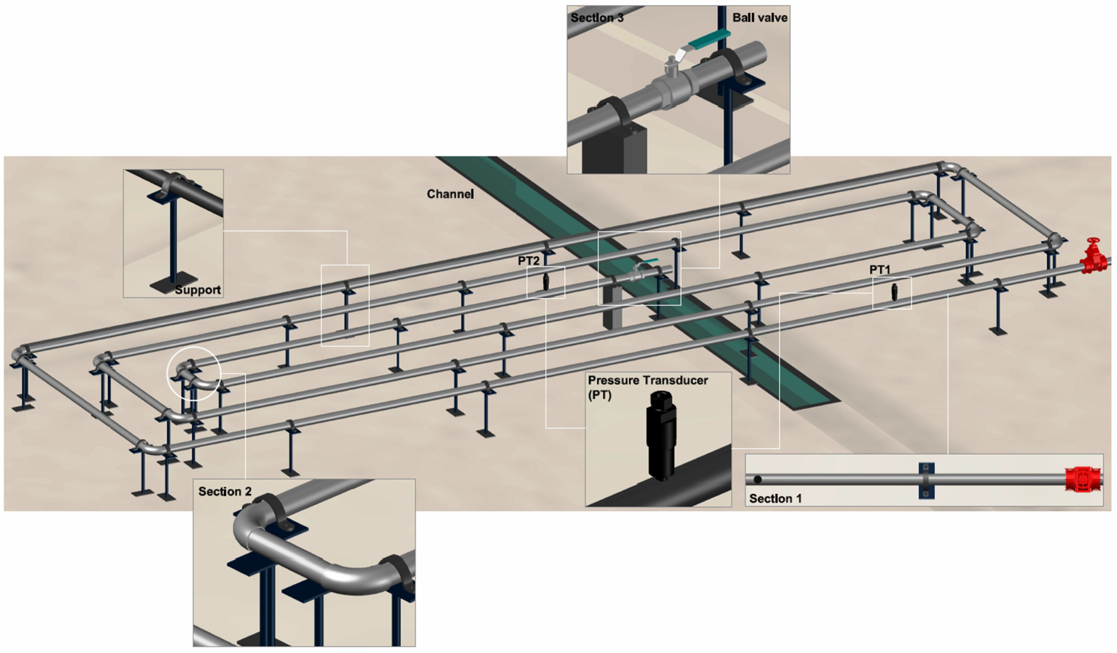
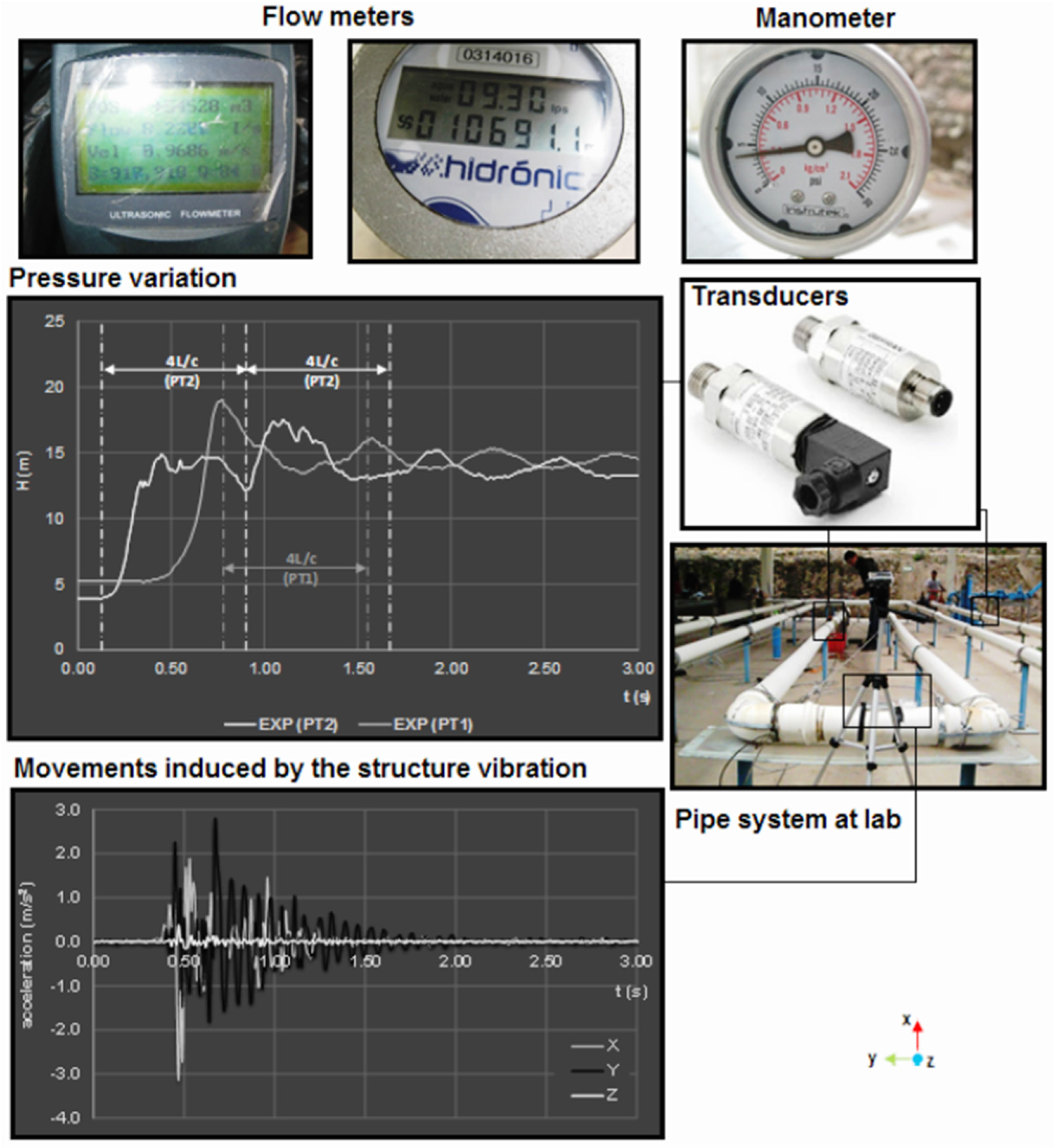
2. Experimental Study
Laboratory Facility
3. Methods
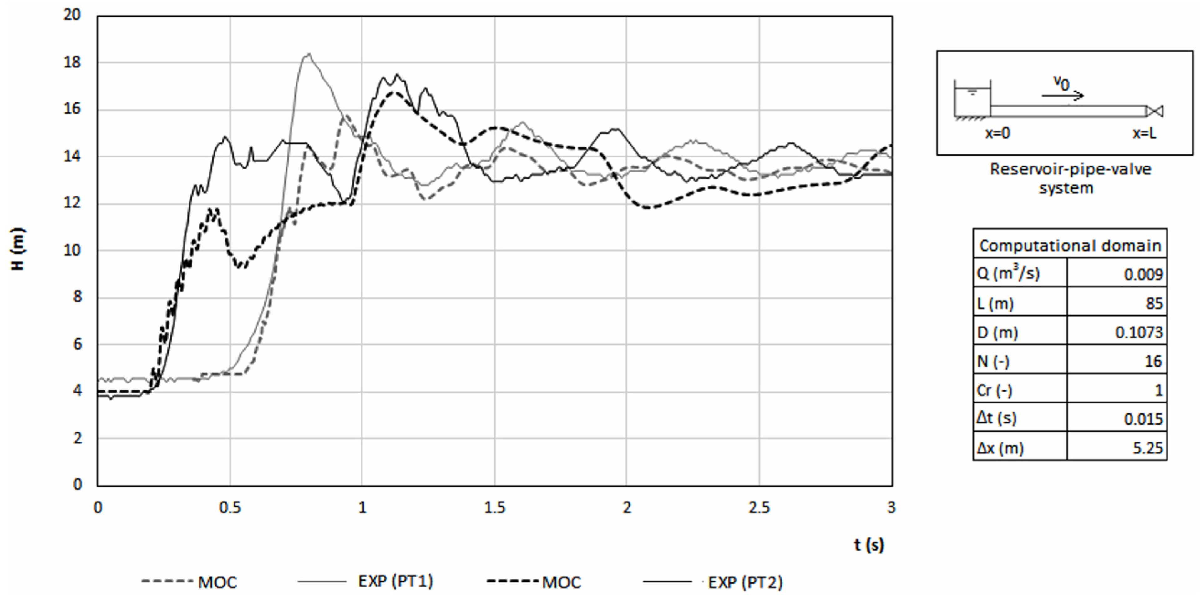
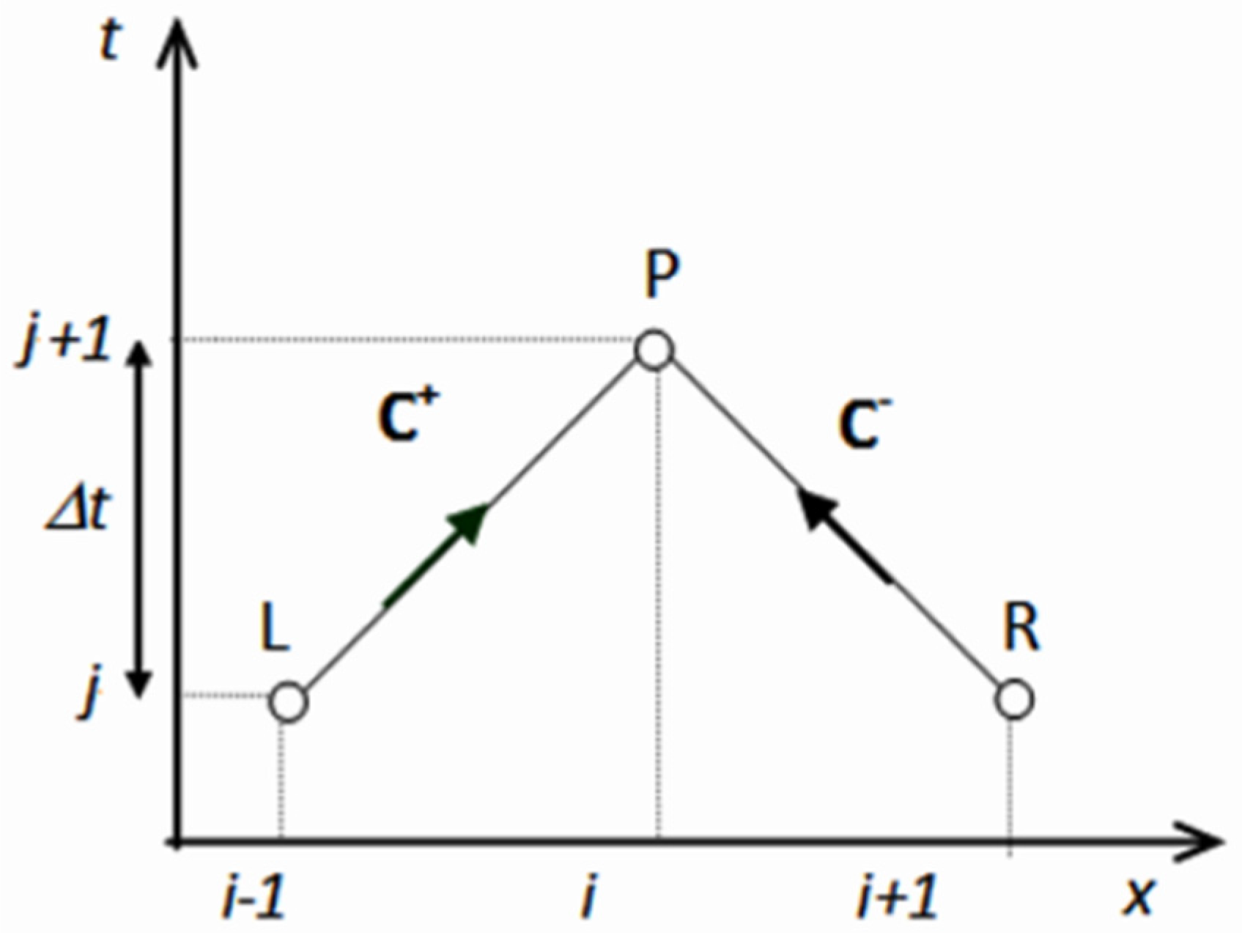
3.1. Modified Method of Characteristic Model with Non-Elastic Effects


| Description | Parameter/Coefficient | Value |
|---|---|---|
| Upstream head (m) | H | 14.4 |
| Discharge (m3/s) | Q | 0.009 |
| Wave speed (m/s) | 350 | |
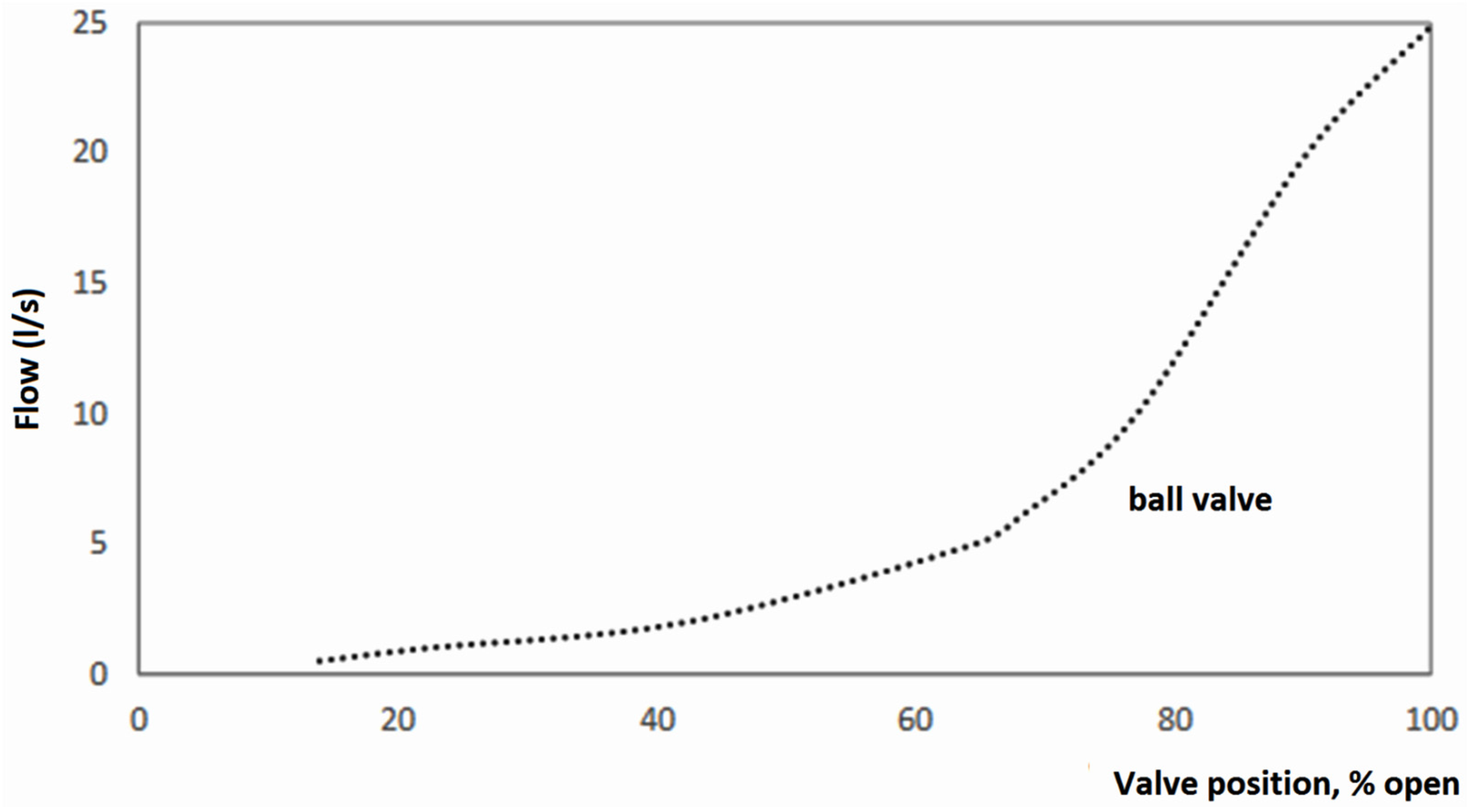
| Time closure of the ball valve (s) | tf | 0.20 |
| Total simulation time (s) | tt | 3 |
| Head coefficient induced by a discharge variation by non-elastic fluid and pipe deformation (--) | KH | 0.32 |
| Discharge coefficient induced by a head variation, due to a non-elastic response in the recuperation phase of the deformation (--) | KQ | 2.9 |
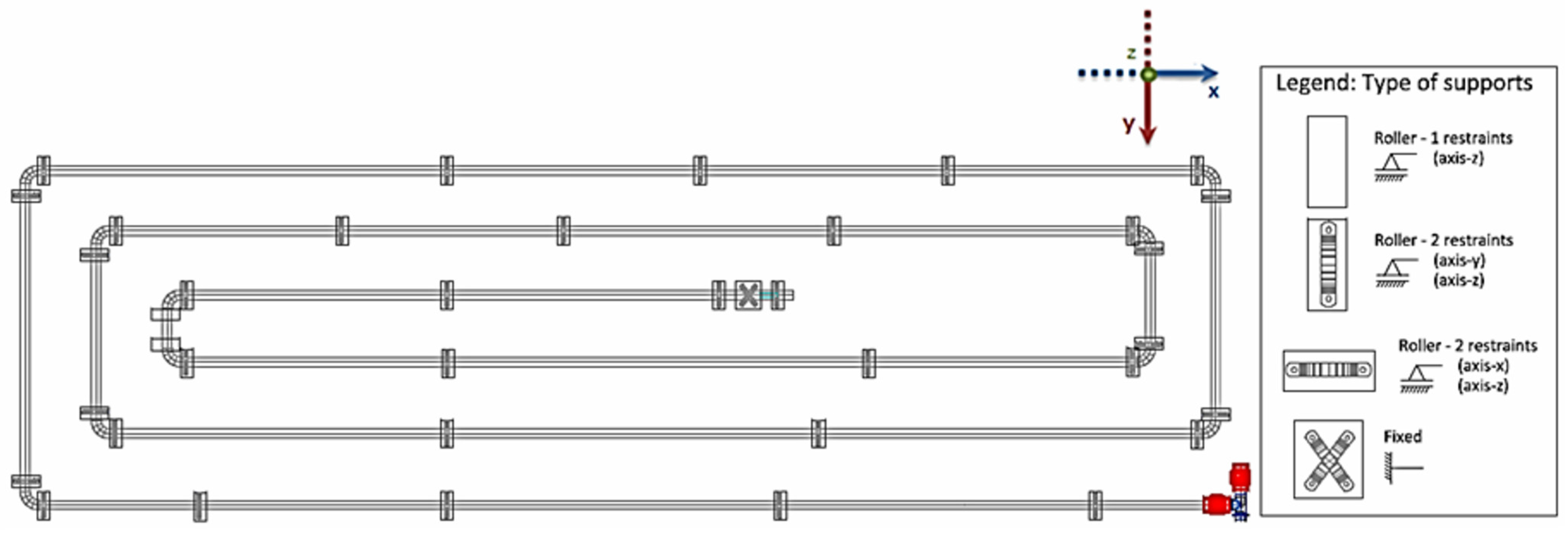
| Support Conditions | Non-Dimensional Parameter () |
|---|---|
| Pipe with frequent expansion joints | |
| Pipe against longitudinal movement throughout its length | |
| Pipe against longitudinal movement at the upper end |
| Material | PVC | ||
|---|---|---|---|
| Di (m) | 0.107 | ||
| e (m) | 0.0035 | ||
| E (GPa) | 2.98 | ||
| K (N/m2) | 2.19 × 10⁹ | ||
| (kg/m3) | 1000 | ||
| (--) | 0.46 | ||
| 1 | 0.79 | 0.77 | |
| c (m/s) | 300 | 350 | 350 |
| wave speed adopted (m/s) | 350 | ||
3.2. FSI Modeling and Solution
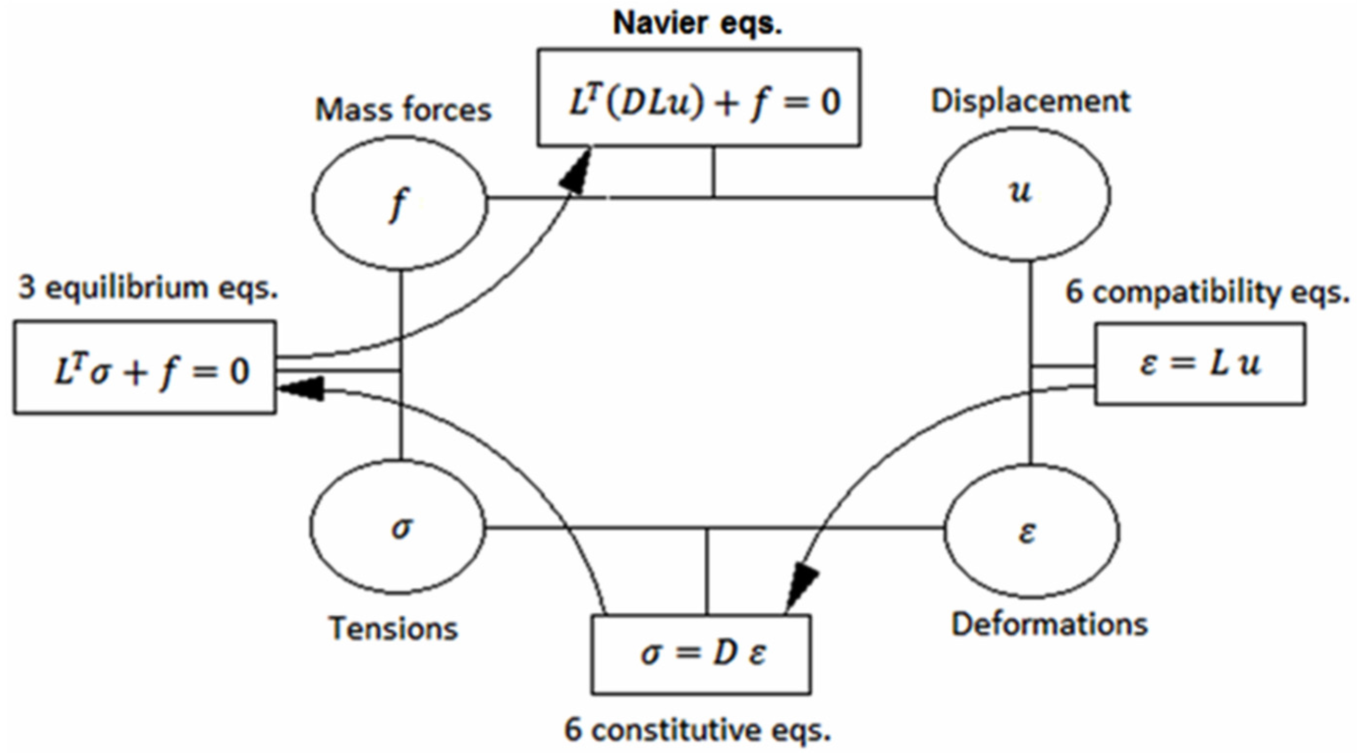
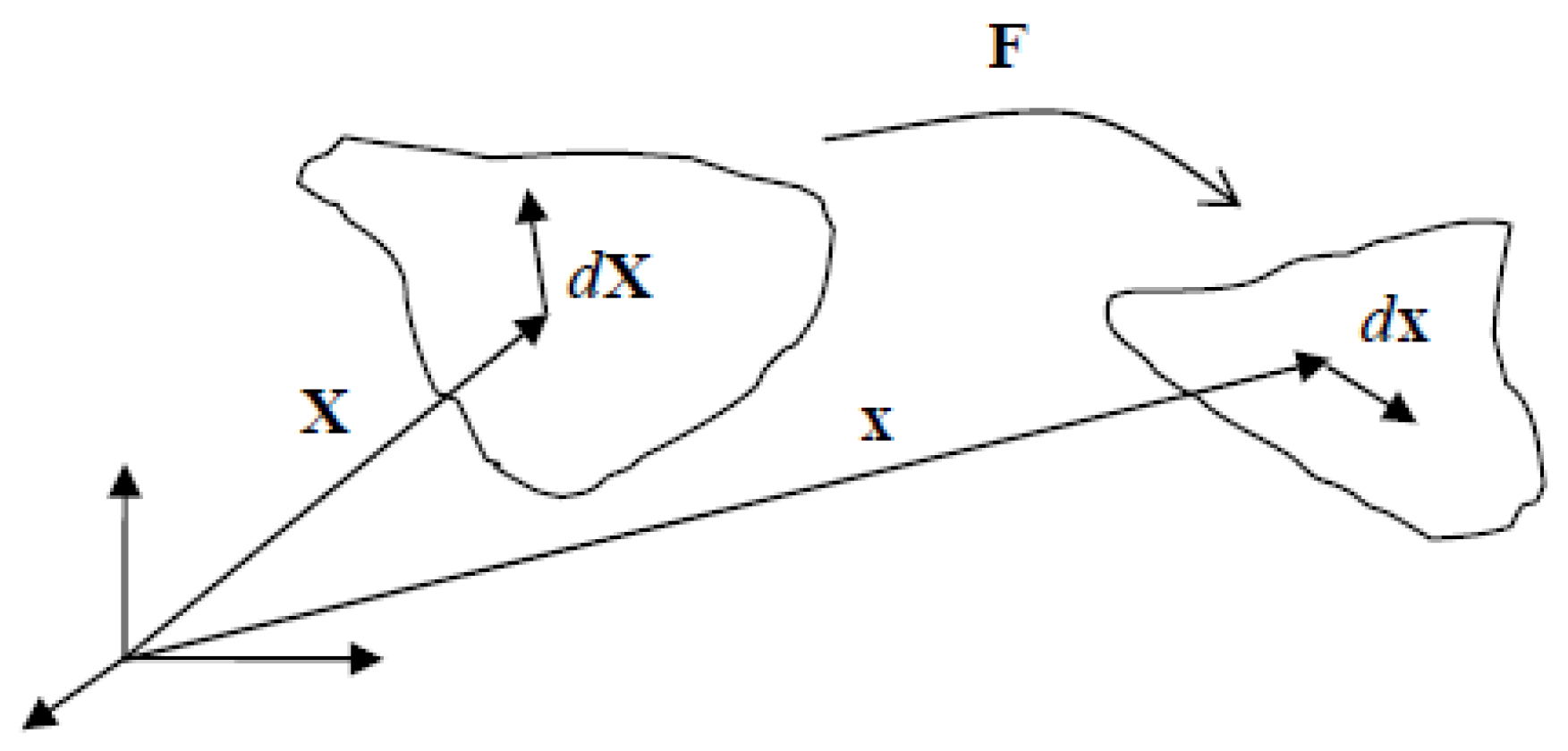
3.2.1. Basic Concepts

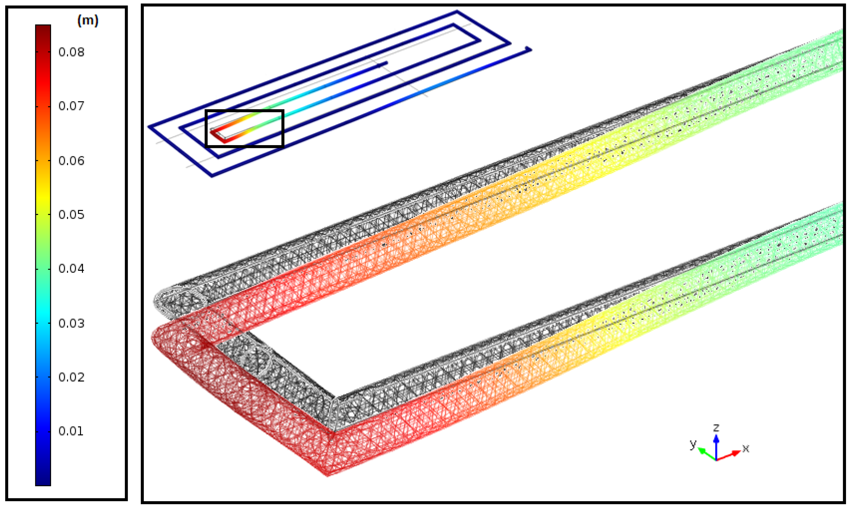
3.2.2. Geometry and Mesh Adaptation


3.2.3. Boundary Conditions


4. Results
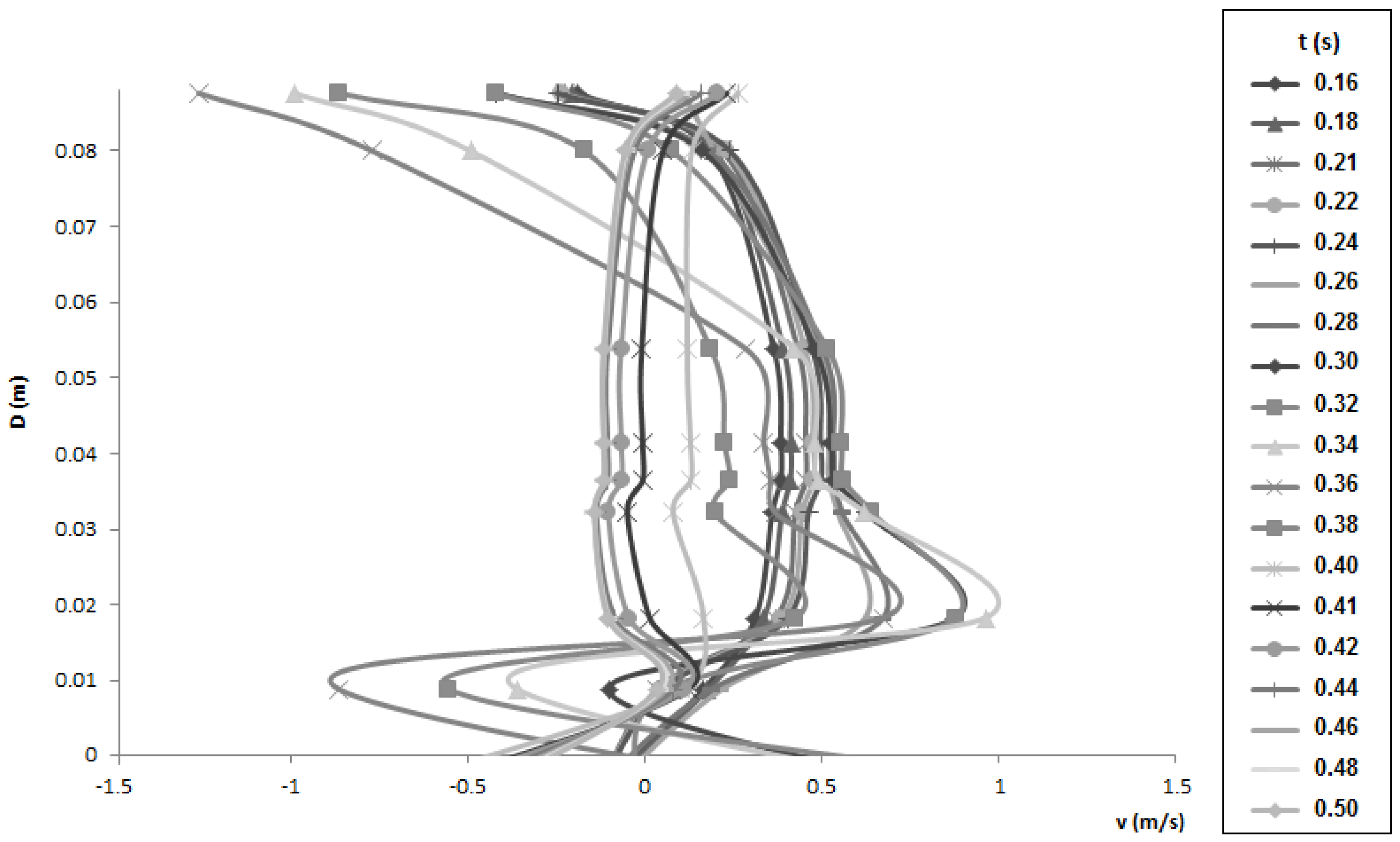
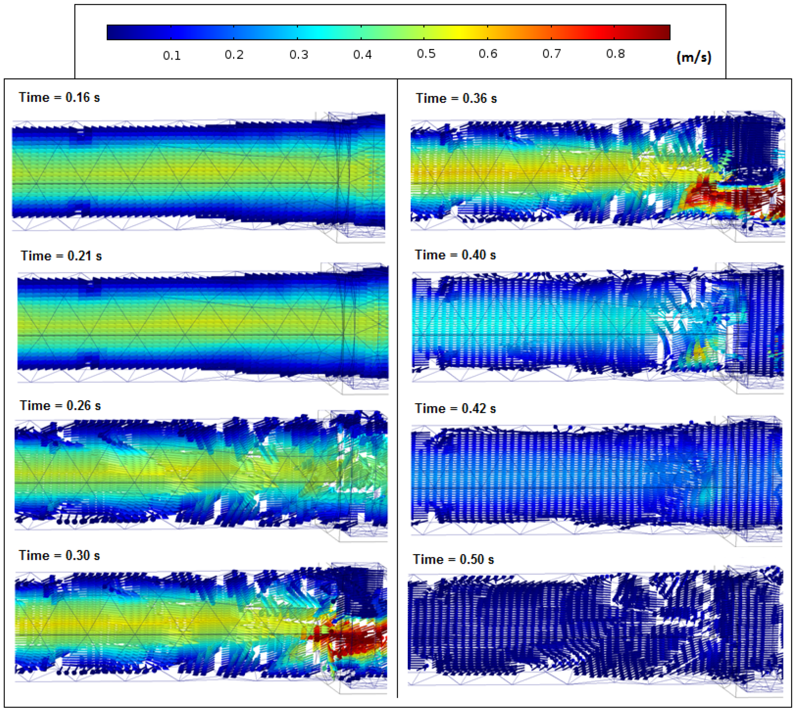
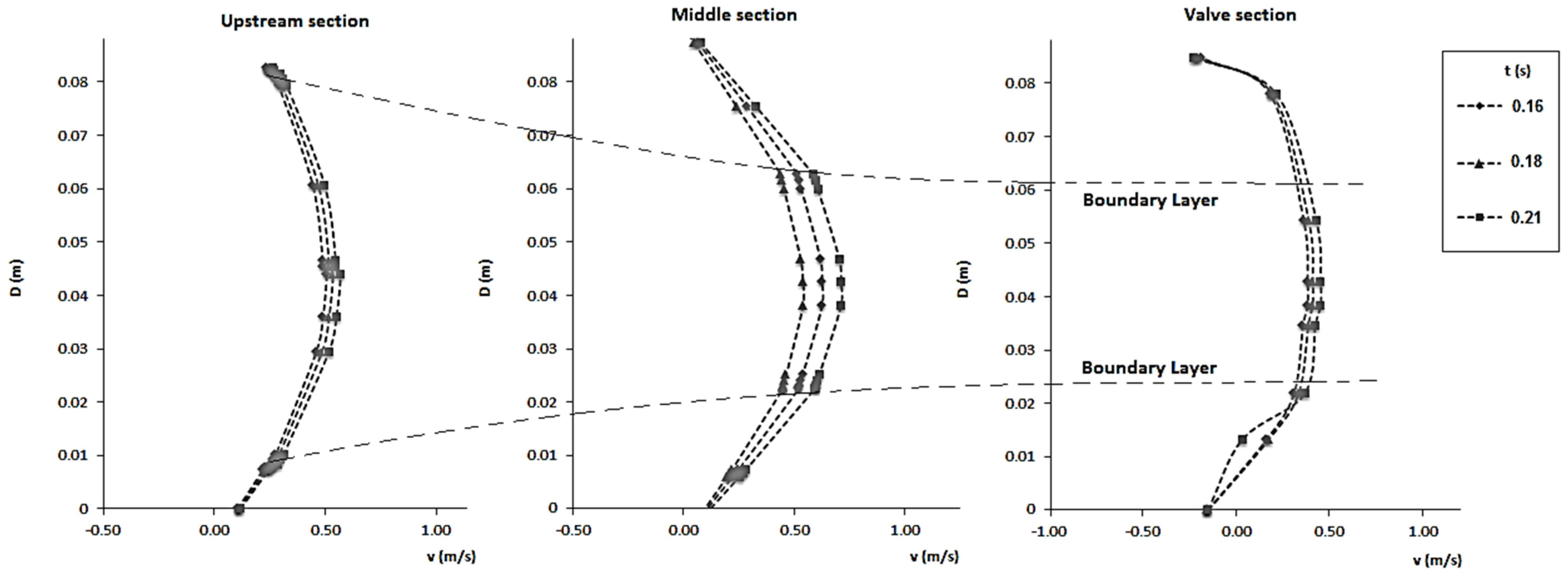
4.1. Velocity Profiles


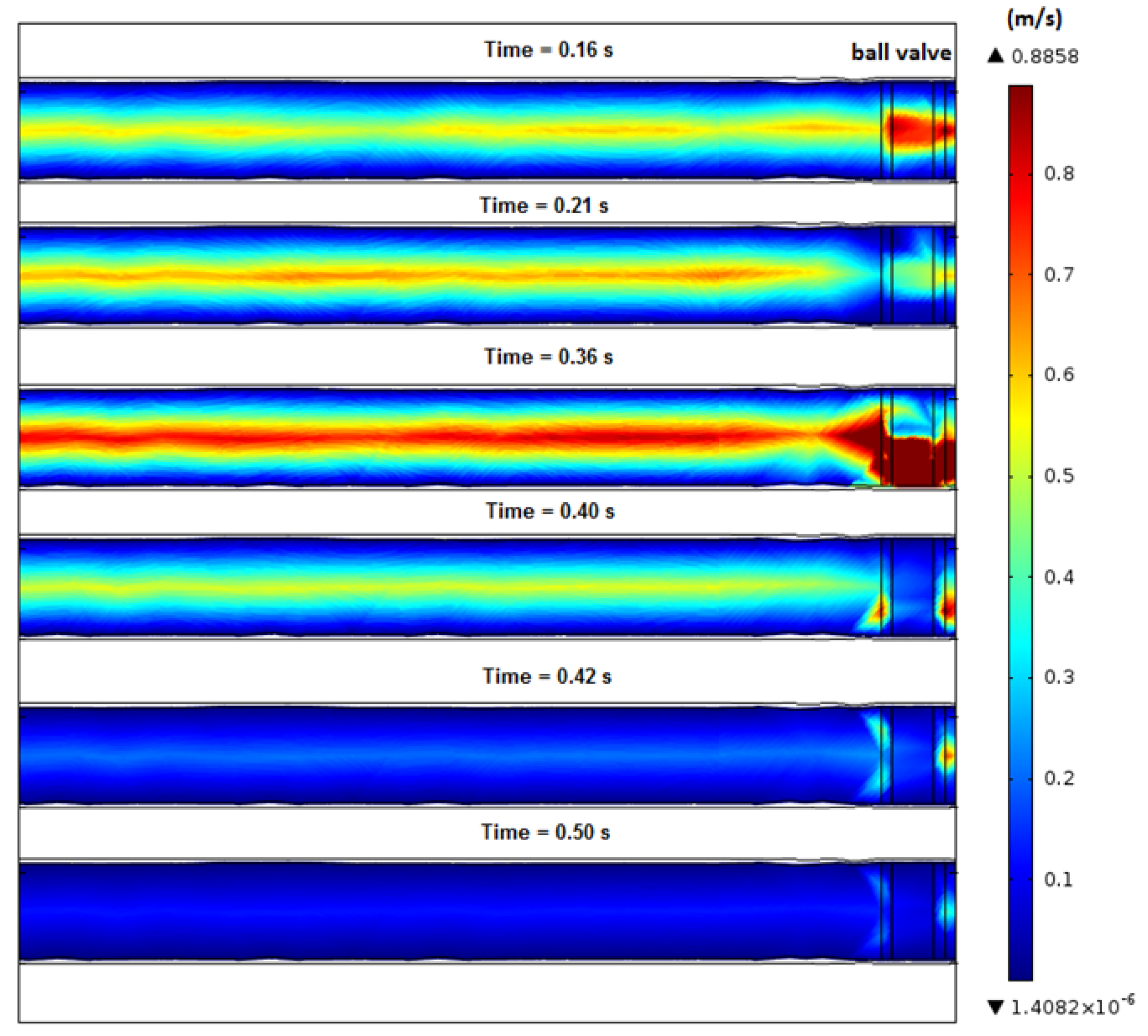
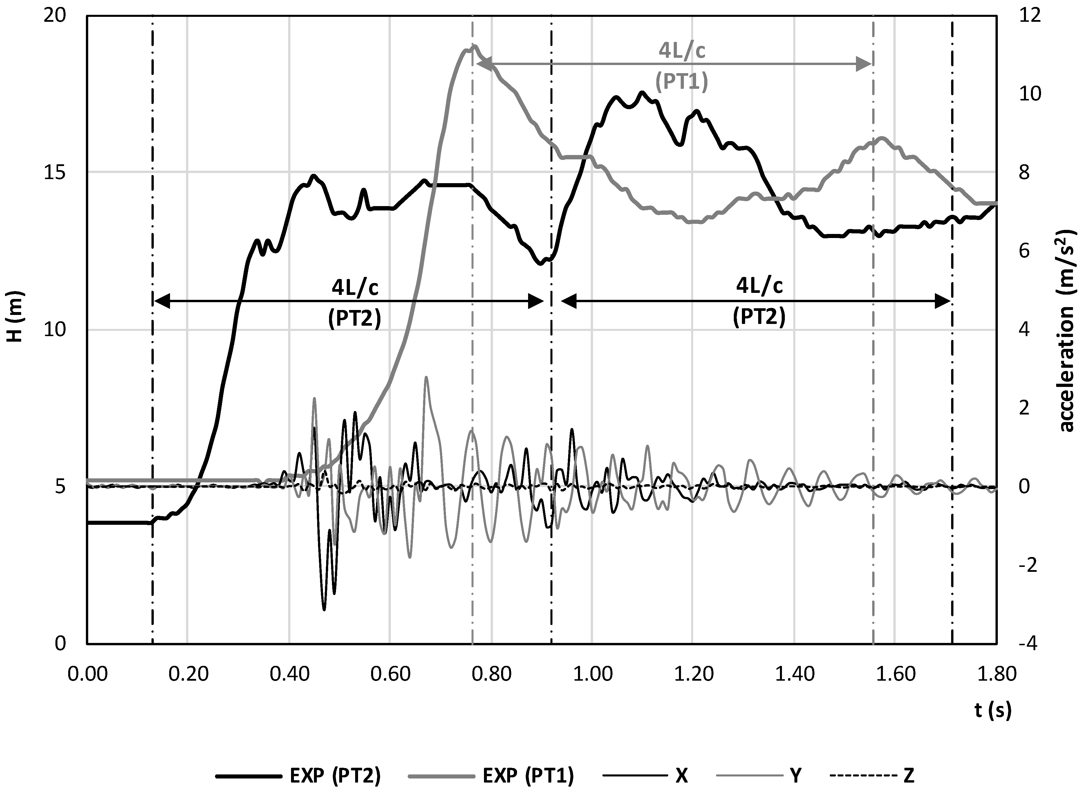
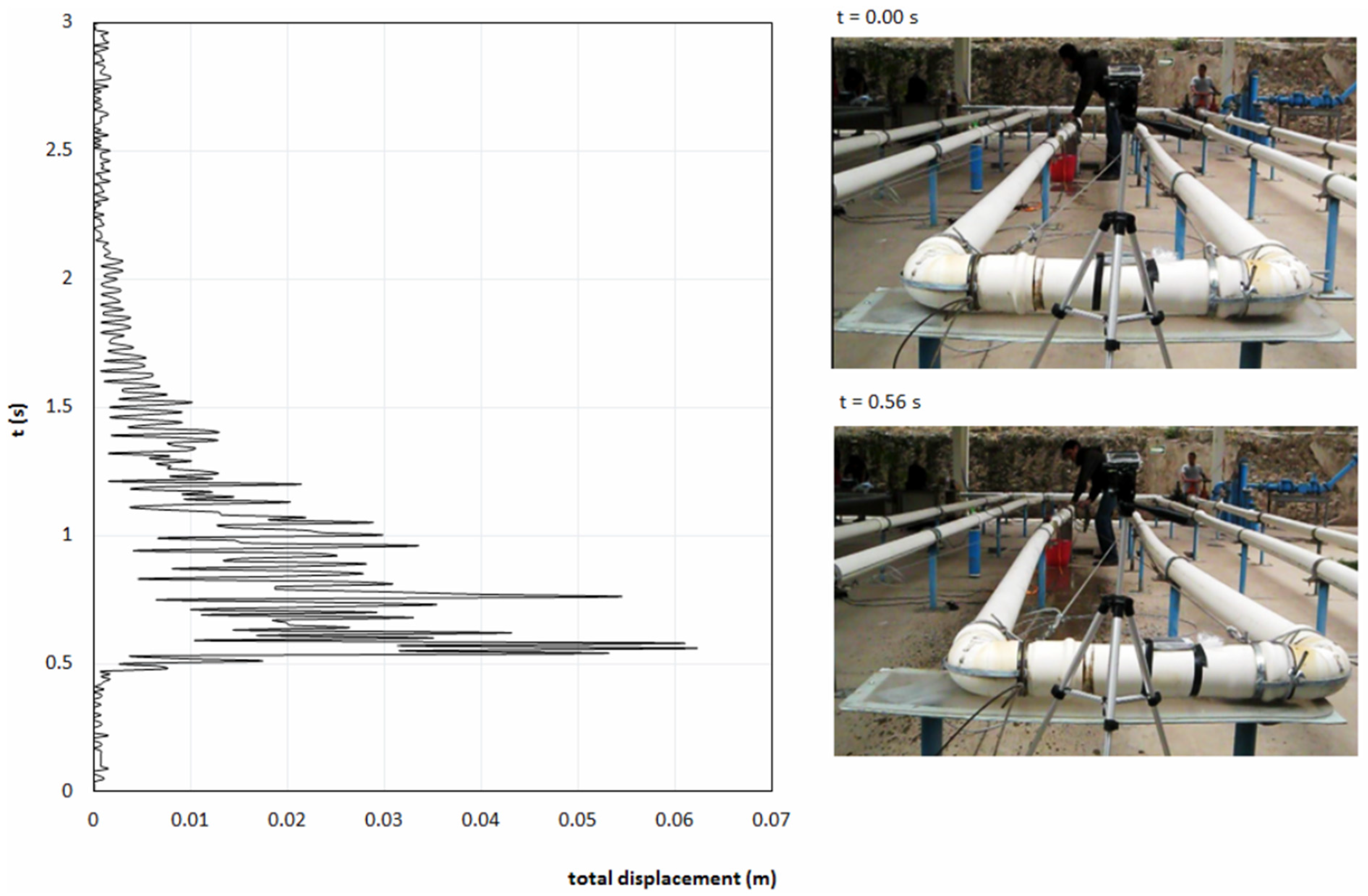
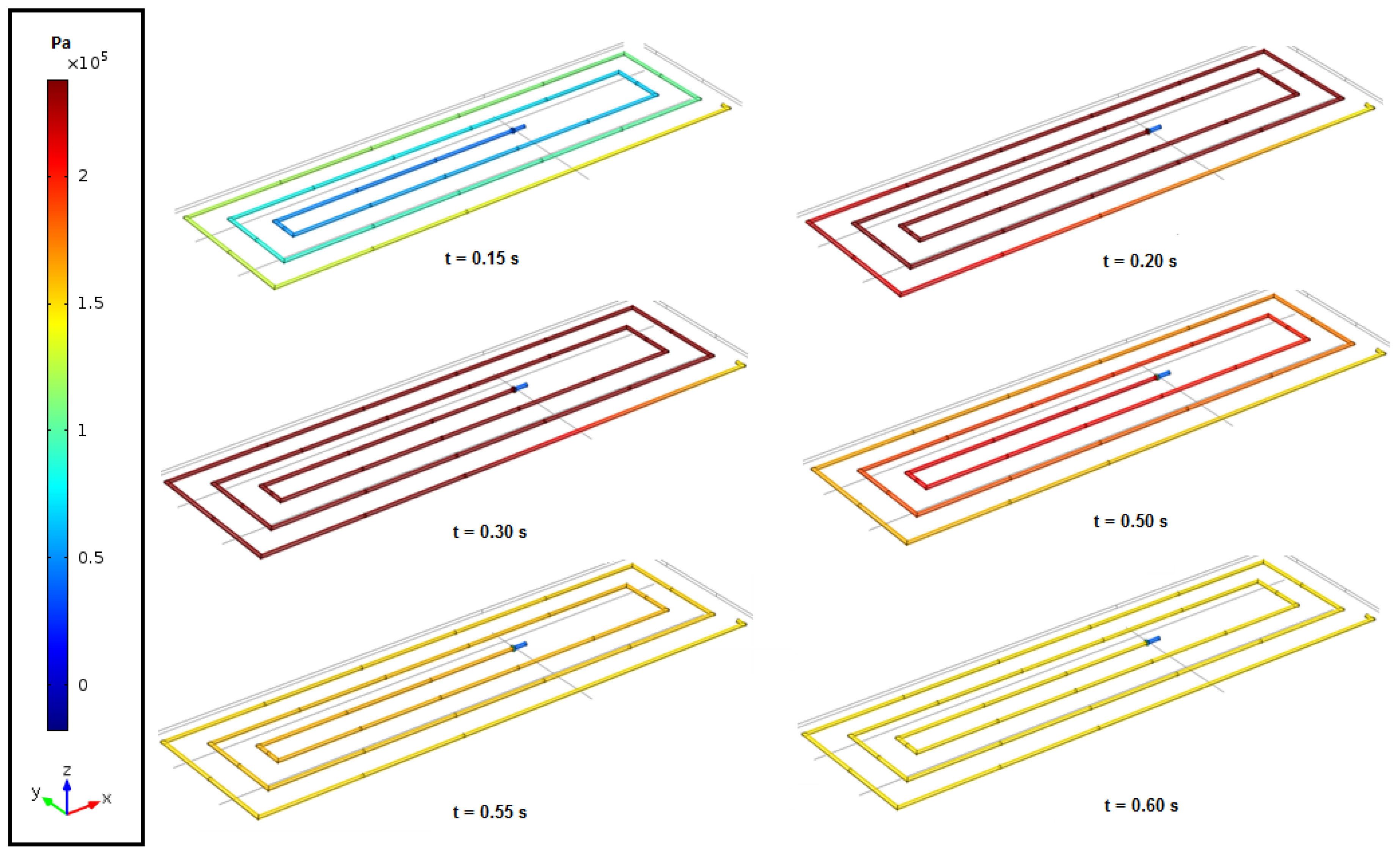
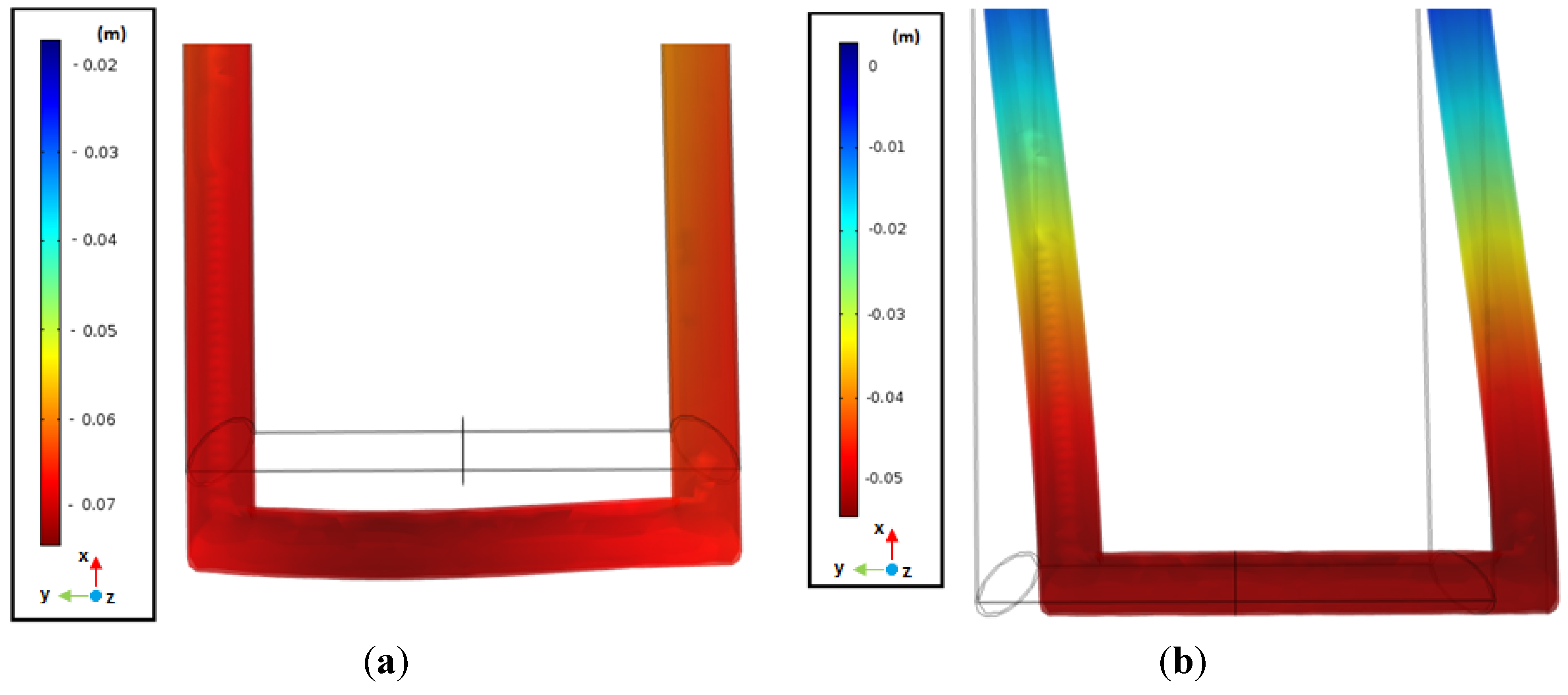
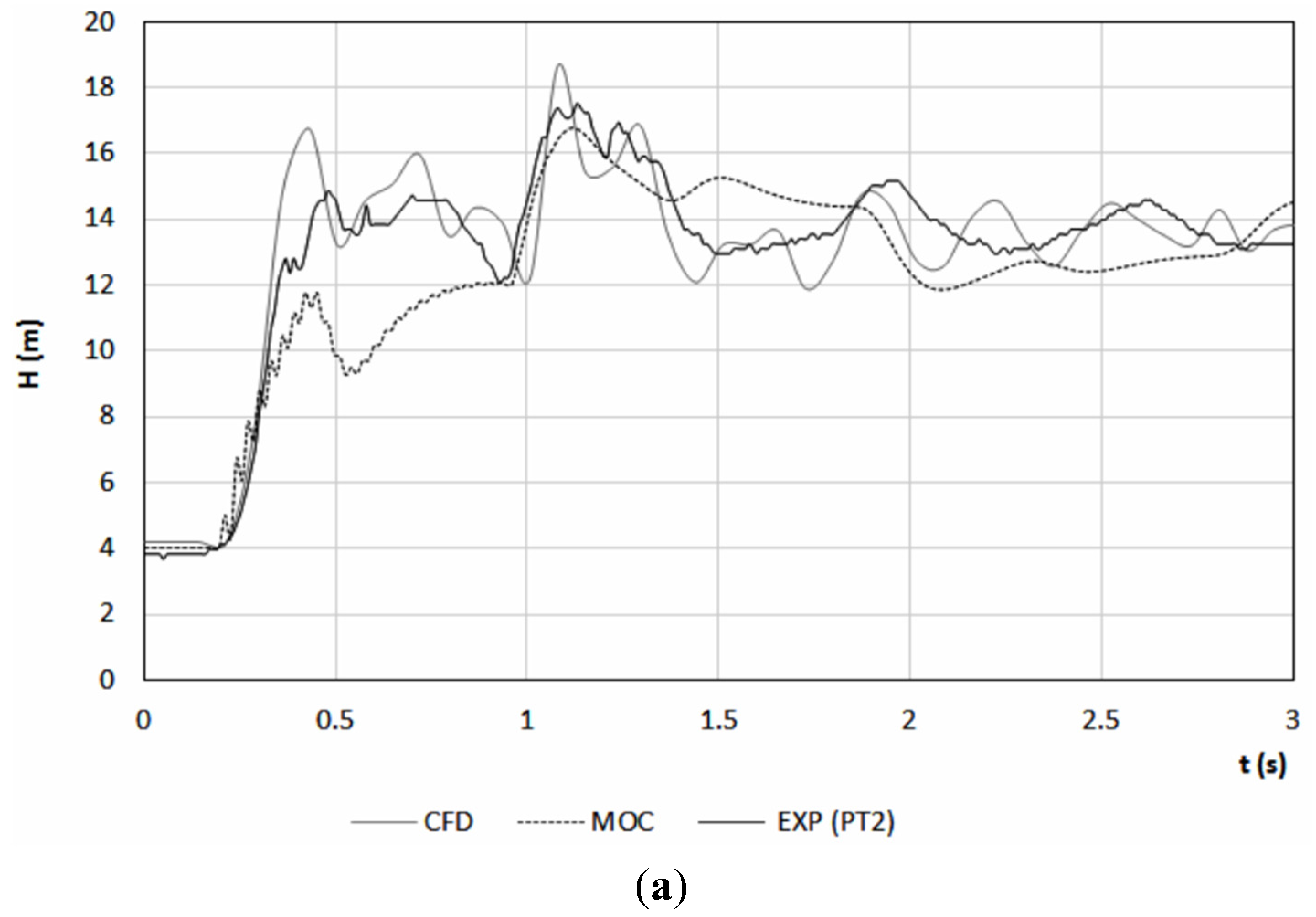
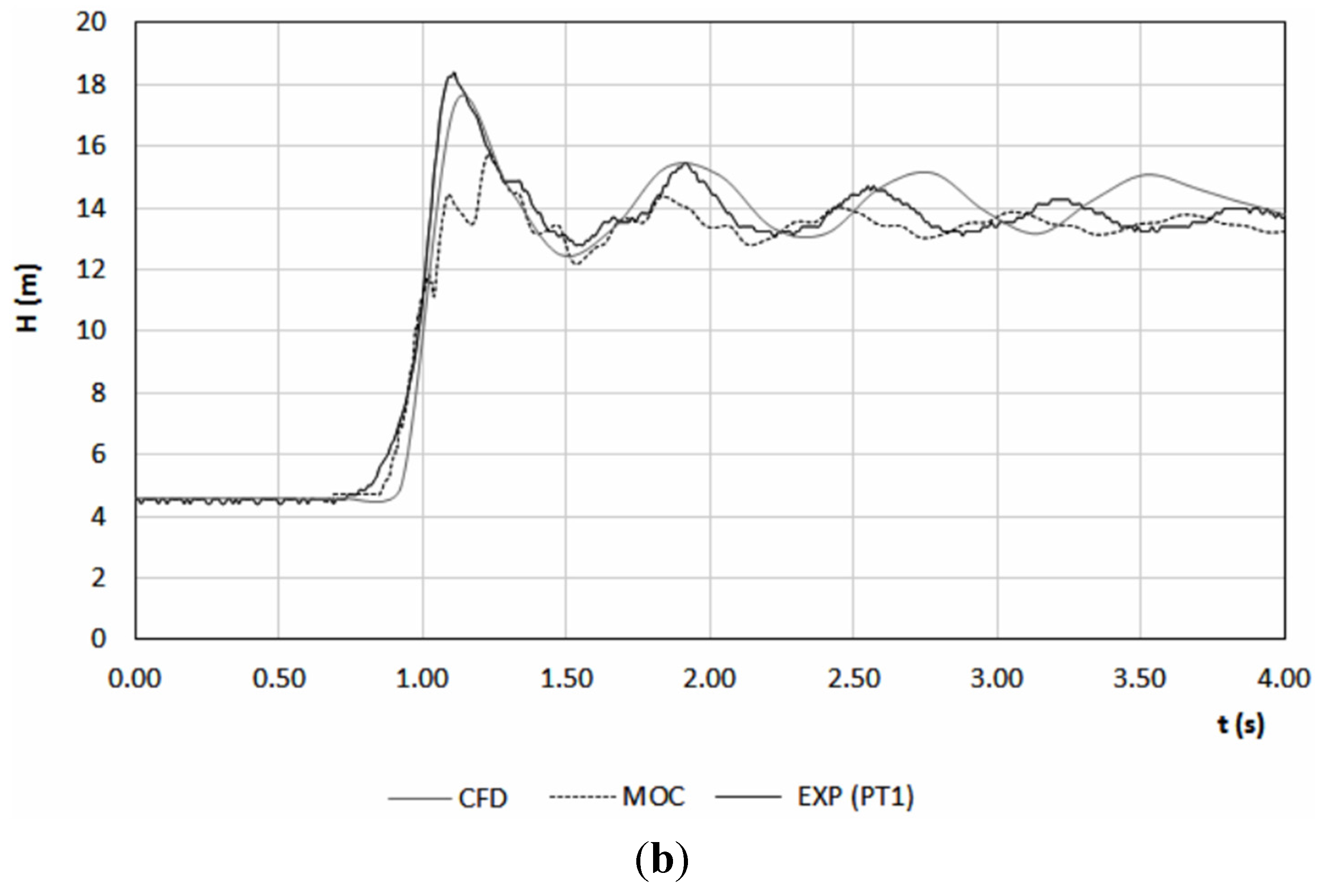
4.2. Wave Propagation and Pipe Displacements

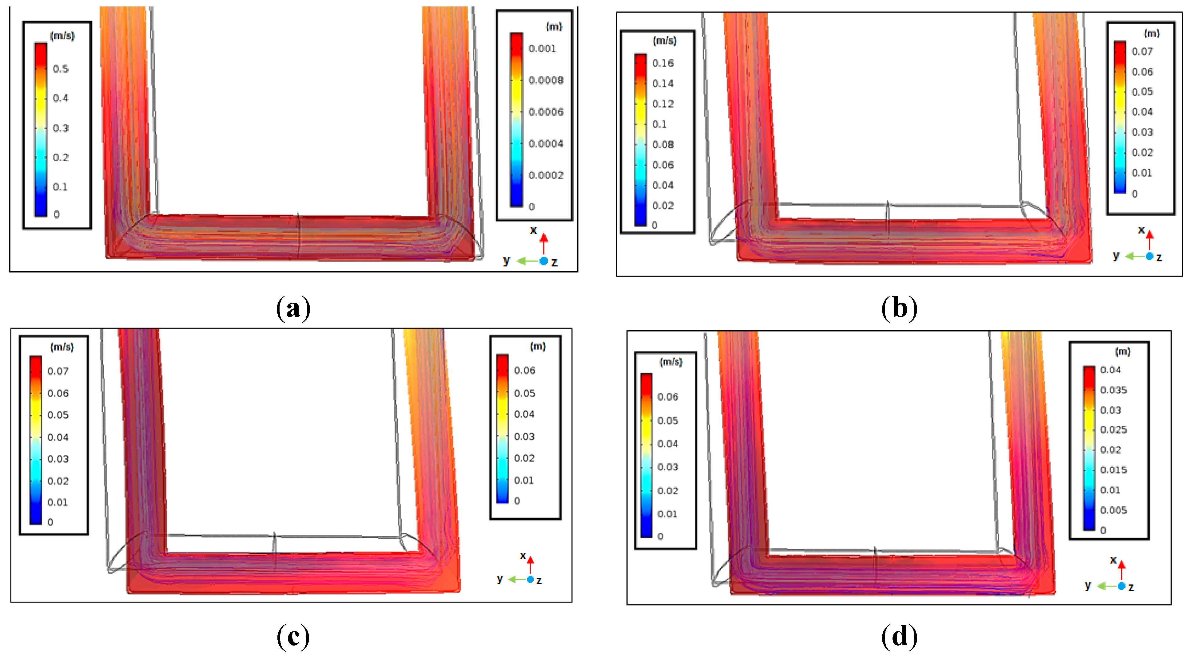

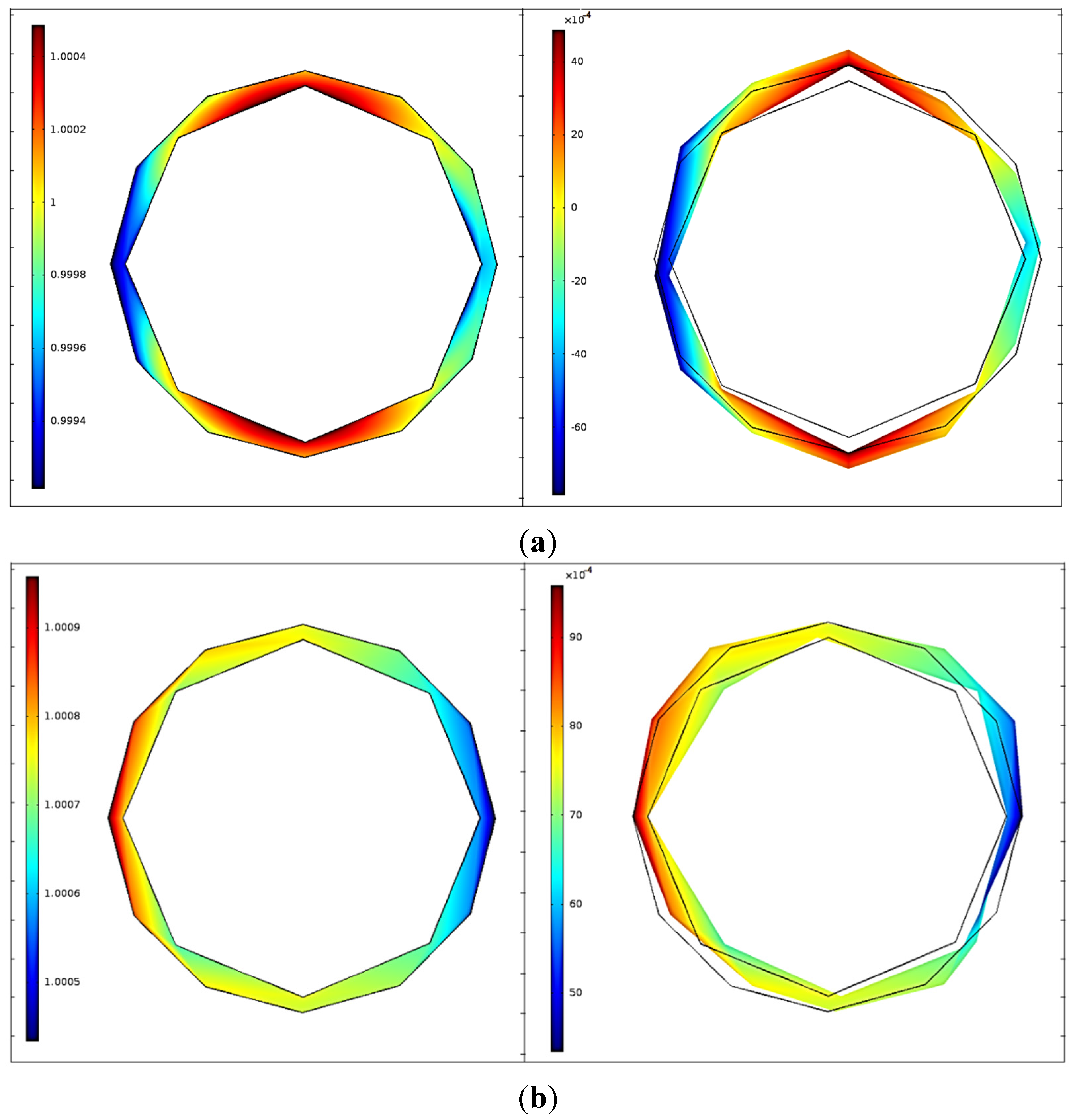
4.3. Deformation Gradient


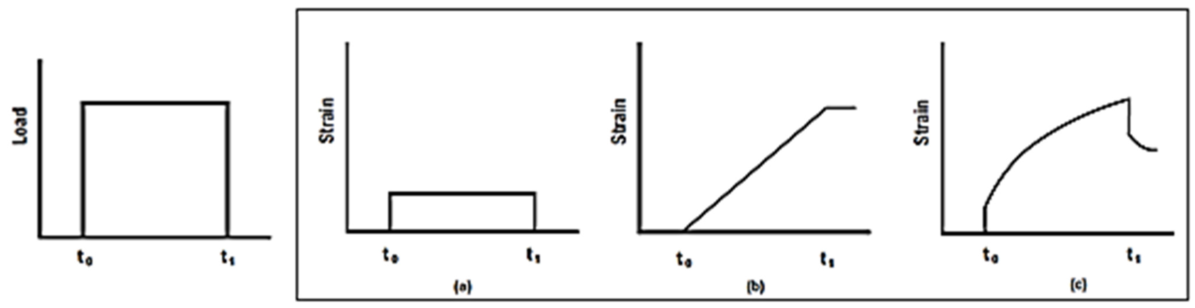
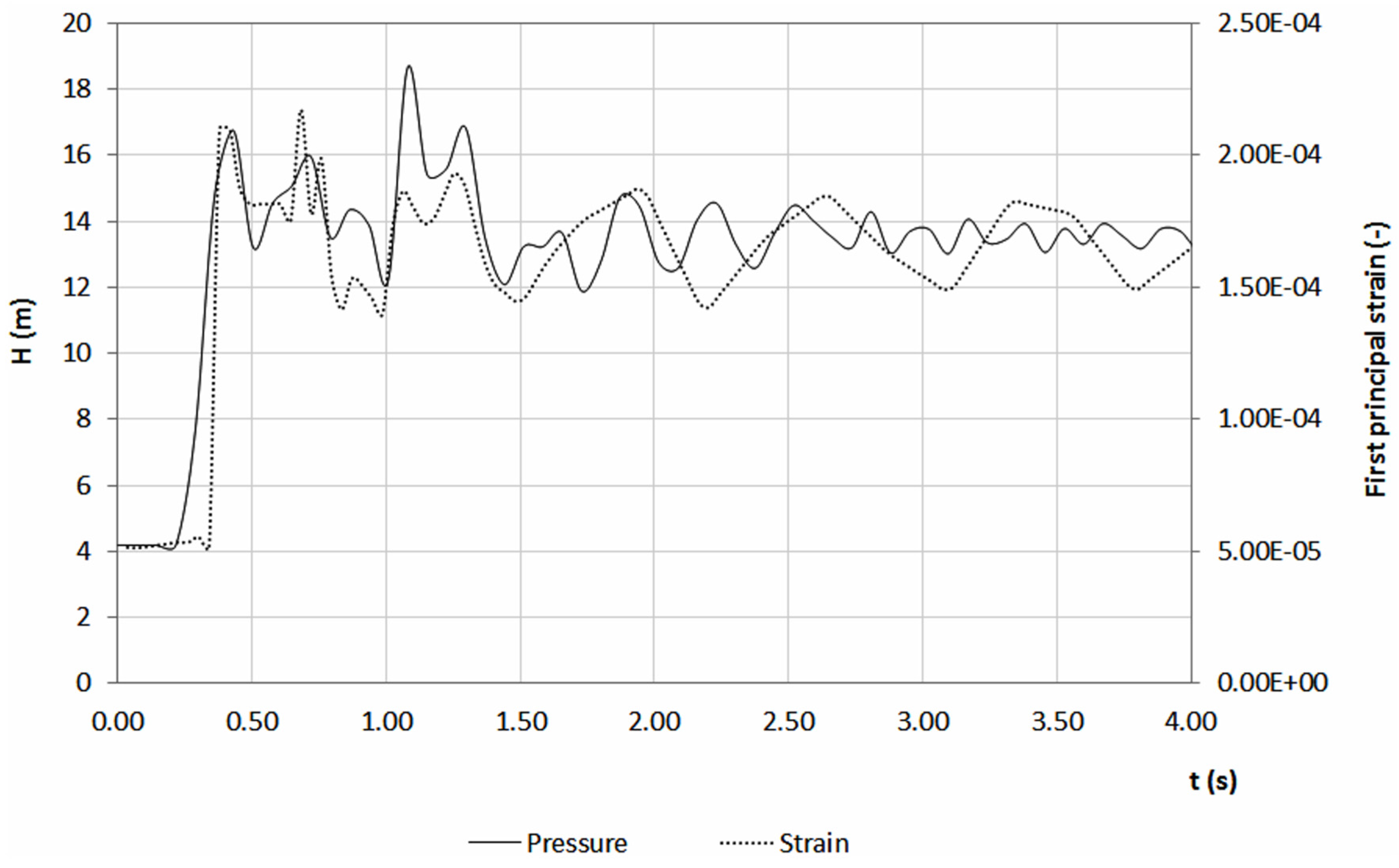
4.4. Stress/Strain Response

5. Discussion


| Parameter | Experimental Data | MOC Model | CFD Model |
|---|---|---|---|
| (m) | 18.2 | 16.0 | 17.9 |
| (m) | 17.5 | 17.0 | 19.0 |
| (m) | 0.063 | -- | 0.087 |
| (m) | 0.037 | -- | 0.051 |
| (m) | 0.053 | -- | 0.071 |
| Relative error (of pressure) | 12% | 8% | |

6. Conclusions
Acknowledgments
Author Contributions
Conflicts of Interest
References
- Bathe, K.J.; Wilson, E.L.; Peterson, F.E. SAPIV—A Structural Analysis Program for Static and Dynamic Response of Linear Systems; Department of Civil Engineering, University of California: Berkeley, CA, USA, 1973. [Google Scholar]
- Lüdecke, H.J.; Kothe, B. Water hammer. In Communications; Aktiengesellschaft, K.S.B., Ed.; Know-How: Halle, Germany, 2006. [Google Scholar]
- Turki, A. Modeling of Hydraulic Transients in Closed Conduits. Master’s Thesis, Department of Civil and Environmental Engineering, Fort Collins, CO, USA, 2013. [Google Scholar]
- Casadei, F.; Halleux, J.P.; Sala, A.; Chillè, F. Transient fluid-structure interaction algorithms for large industrial applications. Comput. Methods Appl. Mech. Eng. 2001, 190, 3081–3110. [Google Scholar] [CrossRef]
- Wiggert, D.C.; Tijsseling, A.S. Fluid Transients and Fluid-Structure Interaction in Flexible Piping Systems. Reports on Applied and Numerical Analysis; Department of Mathematics and Computing Science, Eindhoven University of Technology: Eindhoven, The Netherlands, 2001. [Google Scholar]
- Wiggert, D.C.; Tijsseling, A.S. Fluid transients and fluid-structure interaction in flexible liqui-filled piping. Appl. Mech. Rev. 2001, 54, 455–481. [Google Scholar] [CrossRef]
- Tijsseling, A.S. Fluid-Structure Interaction in Liquid-Filled Pipe Systems. J. Fluids Struct. 1996, 10, 109–146. [Google Scholar] [CrossRef]
- Almeida, A.B.; Pinto, A.A.M. A special case of transient forces on pipeline supports due to water hammer effects. In Proceedings of the 5th International Conference on Pressure Surges, Hanover, Germany, 22–24 September 1986; pp. 27–34.
- Obradovíc, P. Fluid-Structure interactions: An accident which has demostrated the necessity for FSI analysis. In Proceedings of the 15th IAHR Symposium on Hydraulic Machinery and Cavitation, Belgrade, Yugoslavia, 11–14 September 1990.
- Wang, C.Y.; Pizzica, P.A.; Gvildys, J.; Spencer, B.W. Analysis of fluid-structure interaction and structural response of Chernobyl-4 reactor. In Proceedings of the SMiRT10, Anaheim, CA, USA, 22–27 August 1989; pp. 109–119.
- Chaudhry, M.H. Applied Hydraulic Transients; Van Nostrand Reinhold Company: New York, NY, USA, 1979. [Google Scholar]
- Ramos, H.; Borga, A.; Covas, D.; Loureiro, D. Surge damping analysis in pipe systems: Modelling and experiments. (Effet d’atténuation du coup de bélier dans les systèmes de conduits: Modelation mathematique et experiences). J. Hydraul. Res. 2004, 42, 413–425. [Google Scholar] [CrossRef]
- Chaudhry, M.H.; Holloway, M.B. Stability of Method of Charaterisitcs. In Proceedings of the Hydraulics Division Specialty Conference, American Society of Civil Engineers, Coeur d’Alene, ID, USA, 14–17 August 1984; pp. 216–220.
- Almeida, A.B.; Koelle, E. Fluid Transients in Pipe Networks. In Computational Mechanics Publications; Elsevier Applied Science: Southampton, UK, 1992. [Google Scholar]
- Wylie, E.B.; Streeter, V.L. Fluid Transients in Systems; Prentice-Hall Inc.: Englewood Cliffs, NJ, USA, 1993. [Google Scholar]
- Chaudhry, M.H.; Hussaini, M.Y. Second order explicit methods for water hammer analysis. J. Fluids Eng. 1993, 107, 523–529. [Google Scholar] [CrossRef]
- Ramos, H.M.; Borga, A.; Covas, D.; Almeida, A. Analysis of Surge Effects in Pipe Systems by Air Release/Venting; APRH: Lisbon, Portugal, 2005; pp. 45–55. [Google Scholar]
- Turpin, J.B. Variable step integration coupled with the method of characteristics solution for water-hammer analysis, a case study. In Proceedings of the 52nd Jannaf Propulsion Meeting, Las Vegas, NV, USA, 10–13 May 2004.
- Hou, Q.; Kruisbrink, A.C.H.; Tijsseling, A.S.; Keramat, A. Simulating water hammer with corrective smoothed particle method, BHR Group. In Proceedings of the 11th International Conference on Pressure Surges, Lisbon, Portugal, 24–26 October 2012; pp. 171–187.
- Bughazem, M.B.; Anderson, A. Problems with simple models for damping in unsteady flow. In Proceedings of the 7th International Conference on Pressure Surges and Fluid Transients in Pipelines and Open Channels, 16–18 April 1996; BHR Group Ltd: Harrogate, UK, 1996; pp. 537–549. [Google Scholar]
- Ferreira, A.J.M. Problems of Finite Element in MatLab; Fundação Calouste Gulbenkian: Lisbon, Portugal, 2010. [Google Scholar]
- Timoshenko, S.P.; Goodier, J.N. Theory of Elasticity; McGraw-Hill: Singapore, 1970. [Google Scholar]
- Arienti, M.; Hung, P.; Shepherd, J.E. Alevel set approach to Eulerian-Lagrangian coupling. J. Comput. Phys. 2003, 185, 213–251. [Google Scholar] [CrossRef]
- Bathe, K.J.; Zhang, H. A mesh adaptivity procedure for CFD and fluid-structure interactions. Comput. Struct. 2009, 87, 604–617. [Google Scholar] [CrossRef]
- Simão, M.; Mora-Rodriguez, J.; Ramos, H.M. Fluid–structure interaction with different coupled models. J. Water Supply Res. Technol. AQUA 2015. [Google Scholar] [CrossRef]
- Causin, P.; Gerbeau, J.F.; Nobile, F. Added-mass effect in the design of partitioned algorithms for fluidstructure problems. Comput. Methods Appl. Mech. Eng. 2005, 194, 4506–4527. [Google Scholar] [CrossRef]
- Felippa, C.A.; Park, K.C.; Farhat, C. Partitioned Analysis of Coupled Mechanical Systems. Comput. Methods Appl. Mech. Eng. 2001, 190, 3247–3270. [Google Scholar] [CrossRef]
- Vaassen, J.M.; de Vincenzo, P.; Hirsch, C.; Leonard, B. Strong Coupling Algorithm to Solve Fluid-Structure-Interaction Problems with a Staggered Approach. In Proceedings of the 7th European Symposium on Aerothermodynamics; Ouwehand, L., Ed.; European Space Agency: Noordwijk, The Netherlands, 2011. [Google Scholar]
- Hou, G.; Wang, J.; Layton, A. Numerical Methods for Fluid-Structure Interaction—A Review. Commun. Comput. Phys. 2012, 12, 337–377. [Google Scholar] [CrossRef]
- Nobile, F.; Vergara, C. Partitioned algorithms for fluidstructure interaction problems in haemodynamics. Milan J. Math. 2012, 80, 443–467. [Google Scholar] [CrossRef]
- González, J.A.; Park, K.C.; Lee, I.; Felippa, C.A.; Ohayon, R. Partitioned Vibration Analysis of Internal Fluid-Structure Interaction Problems. Int. J. Numer. Methods Eng. 2012, 92, 268–300. [Google Scholar] [CrossRef]
- Badia, S.; Nobile, F.; Vergara, C. Fluidstructure partitioned procedures based on Robin transmission conditions. J. Comput. Phys. 2008, 227, 7027–7051. [Google Scholar] [CrossRef]
- Forster, C.; Wall, W.; Ramm, E. Artificial added mass instabilities in sequential staggered coupling of nonlinear structures and incompressible viscous flow. Comput. Methods Appl. Mech. Eng. 2007, 196, 1278–1293. [Google Scholar] [CrossRef]
- Steinstrasser, C.E. Método Difusivo de Lax Aplicado na Solução das Equações de Saint Venant; Universidade Federal do Paraná: Curitiba, Brazil, 2005. [Google Scholar]
- Moussou, P.; Lafon, P.; Potapov, S.; Paulhiac, L.; Tijsseling, A. Industrial cases of FSI due to internal flows. In Proceedings of the 9th International Conference on Pressure Surges, Chester, UK, 24–26 March 2004; BHR Group Ltd.: Cranfield, UK, 2004; pp. 167–181. [Google Scholar]
- Budny, D.D. The Influence of Structural Damping on the Internal Fluid Pressure during a Fluid Transient Pipe Flow. Ph.D. Thesis, Department of Civil and Environmental Engineering, Michigan State University, East Lansing, MI, USA, 1988. [Google Scholar]
- Fan, D. Fluid Structure Interactions in Internal Flows. Ph.D. Thesis, Department of Civil Engineering, The University of Dundee, Dundee, UK, 1989. [Google Scholar]
- Greenshields, C.J.; Weller, H.G.; Ivankovic, A. The finite volume method for coupled fluid flow and stress analysis. Comput. Model. Simul. Eng. 1999, 4, 213–218. [Google Scholar]
© 2015 by the authors; licensee MDPI, Basel, Switzerland. This article is an open access article distributed under the terms and conditions of the Creative Commons Attribution license (http://creativecommons.org/licenses/by/4.0/).
Share and Cite
Simão, M.; Mora-Rodriguez, J.; Ramos, H.M. Mechanical Interaction in Pressurized Pipe Systems: Experiments and Numerical Models. Water 2015, 7, 6321-6350. https://doi.org/10.3390/w7116321
Simão M, Mora-Rodriguez J, Ramos HM. Mechanical Interaction in Pressurized Pipe Systems: Experiments and Numerical Models. Water. 2015; 7(11):6321-6350. https://doi.org/10.3390/w7116321
Chicago/Turabian StyleSimão, Mariana, Jesus Mora-Rodriguez, and Helena M. Ramos. 2015. "Mechanical Interaction in Pressurized Pipe Systems: Experiments and Numerical Models" Water 7, no. 11: 6321-6350. https://doi.org/10.3390/w7116321