
Remote Sensing Based Analysis of Recent Variations in Water Resources and Vegetation of a Semi-Arid Region


Abstract
:1. Introduction
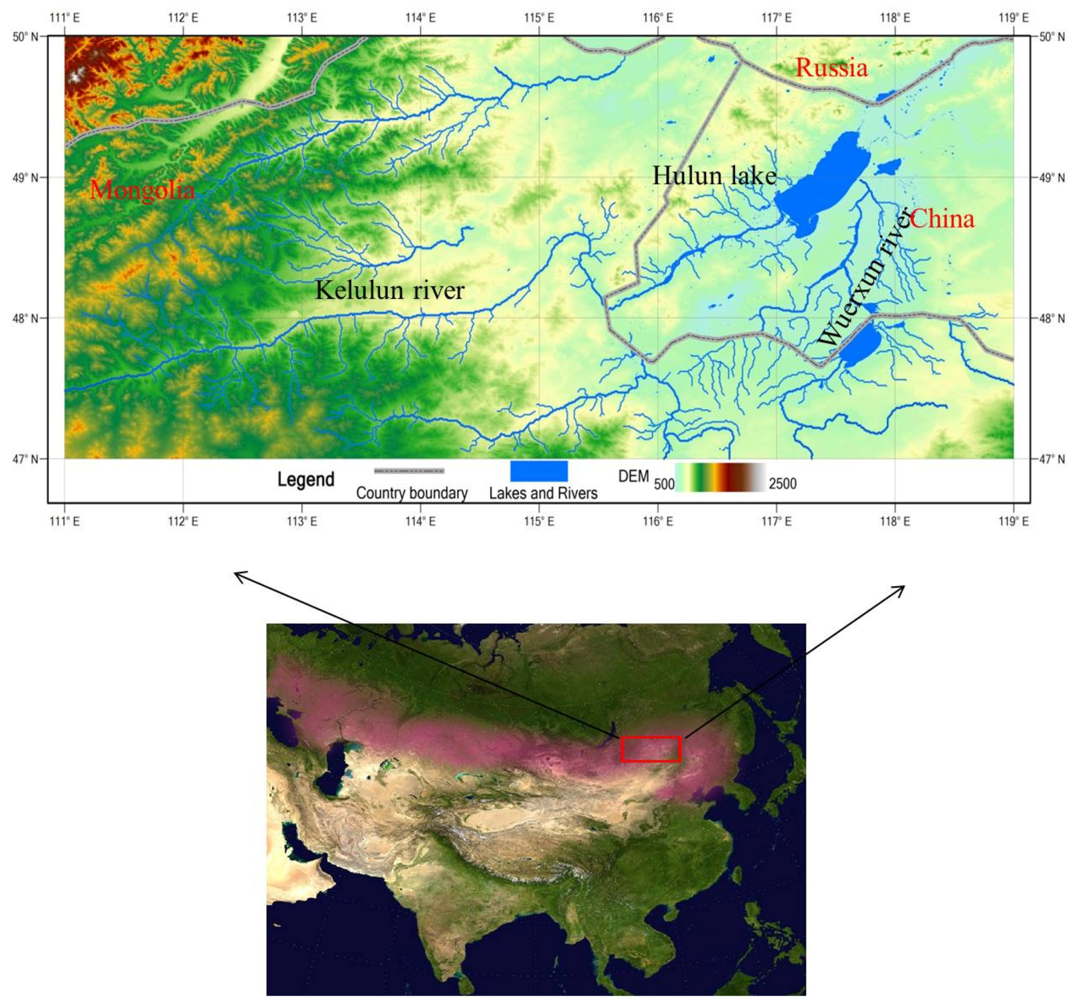
2. Study Area


3. Materials
3.1. Precipitation Data
3.2. Surface Air Temperature Data
3.3. Lake Water Level Data
3.4. Satellite Imagery Data
3.5. GRACE TWS Data
3.6. NDVI Data
4. Methods
4.1. Water Resource Spatial-Temporal Series Analysis
4.2. Lake Water Surface Area Estimation
4.3. NDVI Variation Trend Analysis Method
5. Results and Discussion
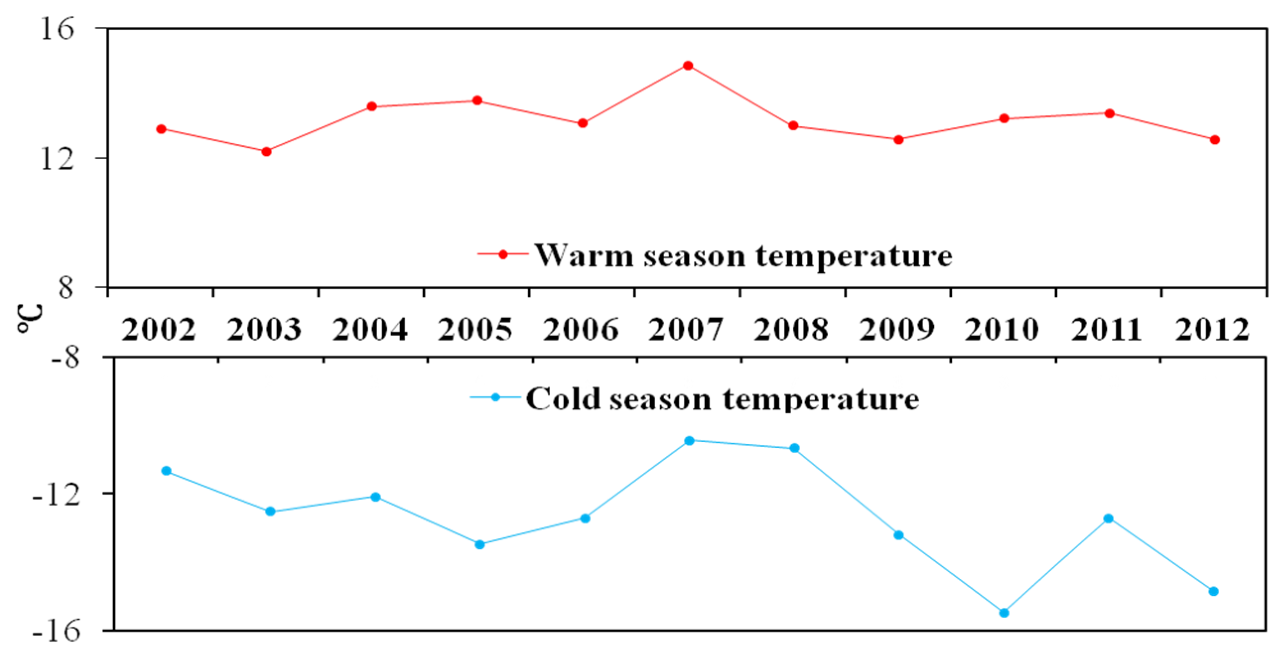
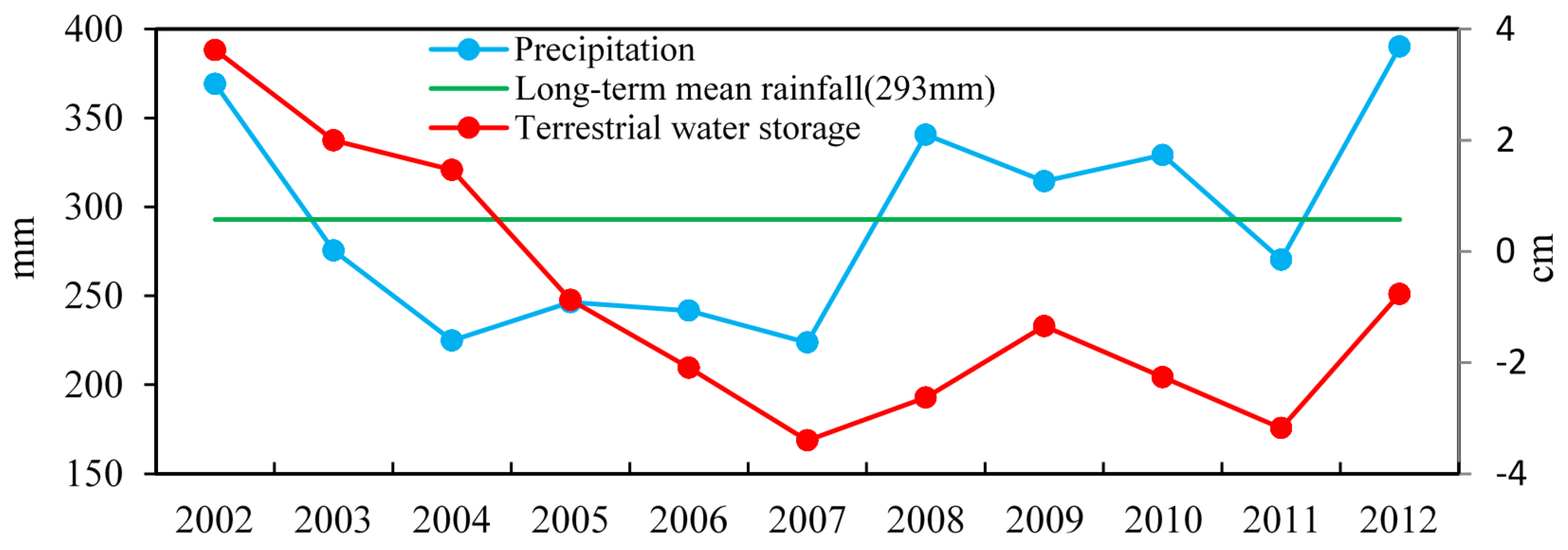
5.1. Precipitation and Temperature Variation Analysis

| No. | Station Name | Latitude | Longitude | R2 |
|---|---|---|---|---|
| 1 | Xinyouqi | 48.67° N | 116.82° E | 0.75 |
| 2 | Xinzuoqi | 48.21° N | 118.27° E | 0.74 |
| 3 | Manzhouli | 49.57° N | 117.43° E | 0.82 |
| 4 | Hailaer | 49.22° N | 119.75° E | 0.92 |
| 5 | Aershan | 47.17° N | 119.93° E | 0.94 |

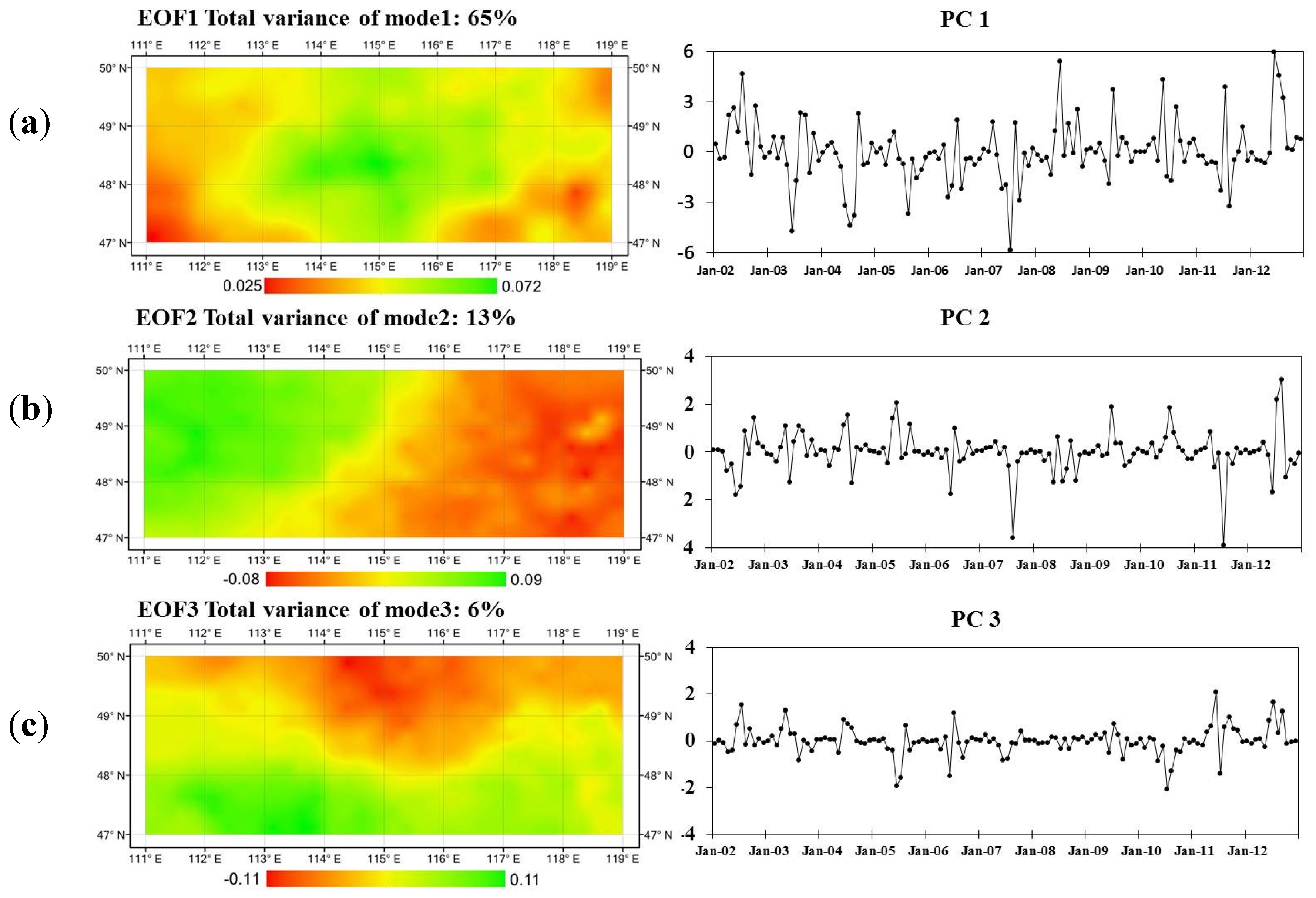
5.2. Water Storage Change

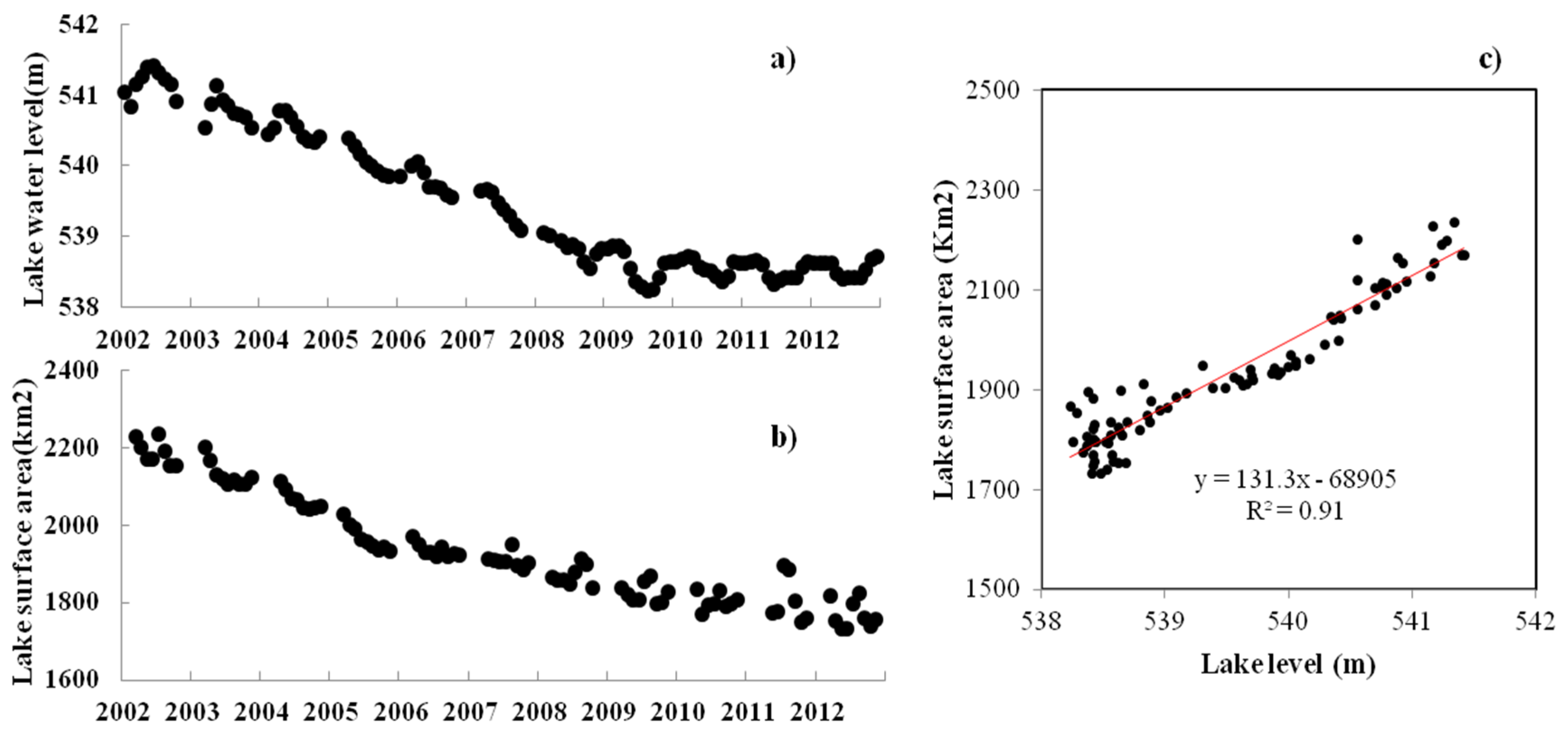
5.3. Lake Response to Water Storage Change
| LANDSAT | MODIS | Absolute Error (km2) | Relative Error (%) | ||
|---|---|---|---|---|---|
| Date | Lake Surface Area (km2) | Date | Lake Surface Area (km2) | ||
| 1 July 2000 | 2306.6 | 4 July 2000 | 2290.1 | −16.4 | −0.71% |
| 6 September 2001 | 2236.4 | 7 September 2001 | 2186.3 | −50.2 | −2.24% |
| 8 August 2002 | 2154.4 | 6 August 2002 | 2221.2 | 66.7 | 3.10% |
| 27 August 2003 | 2114.2 | 30 August 2003 | 2106.9 | −7.3 | −0.35% |
| 13 August 2004 | 2002.5 | 13 August 2004 | 2058.2 | 55.7 | 2.78% |
| 16 August 2005 | 1977.6 | 14 August 2005 | 1948.8 | −28.7 | −1.45% |
| 26 July 2006 | 1938.6 | 29 July 2006 | 1942.9 | 4.3 | 0.22% |
| 29 July 2007 | 1907.2 | 29 July 2007 | 1902.3 | −4.9 | −0.26% |
| 25 August 2008 | 1837 | 13 August 2008 | 1862.1 | 25.1 | 1.36% |
| 5 October 2009 | 1791.5 | 1 October 2009 | 1772.8 | −18.7 | −1.04% |

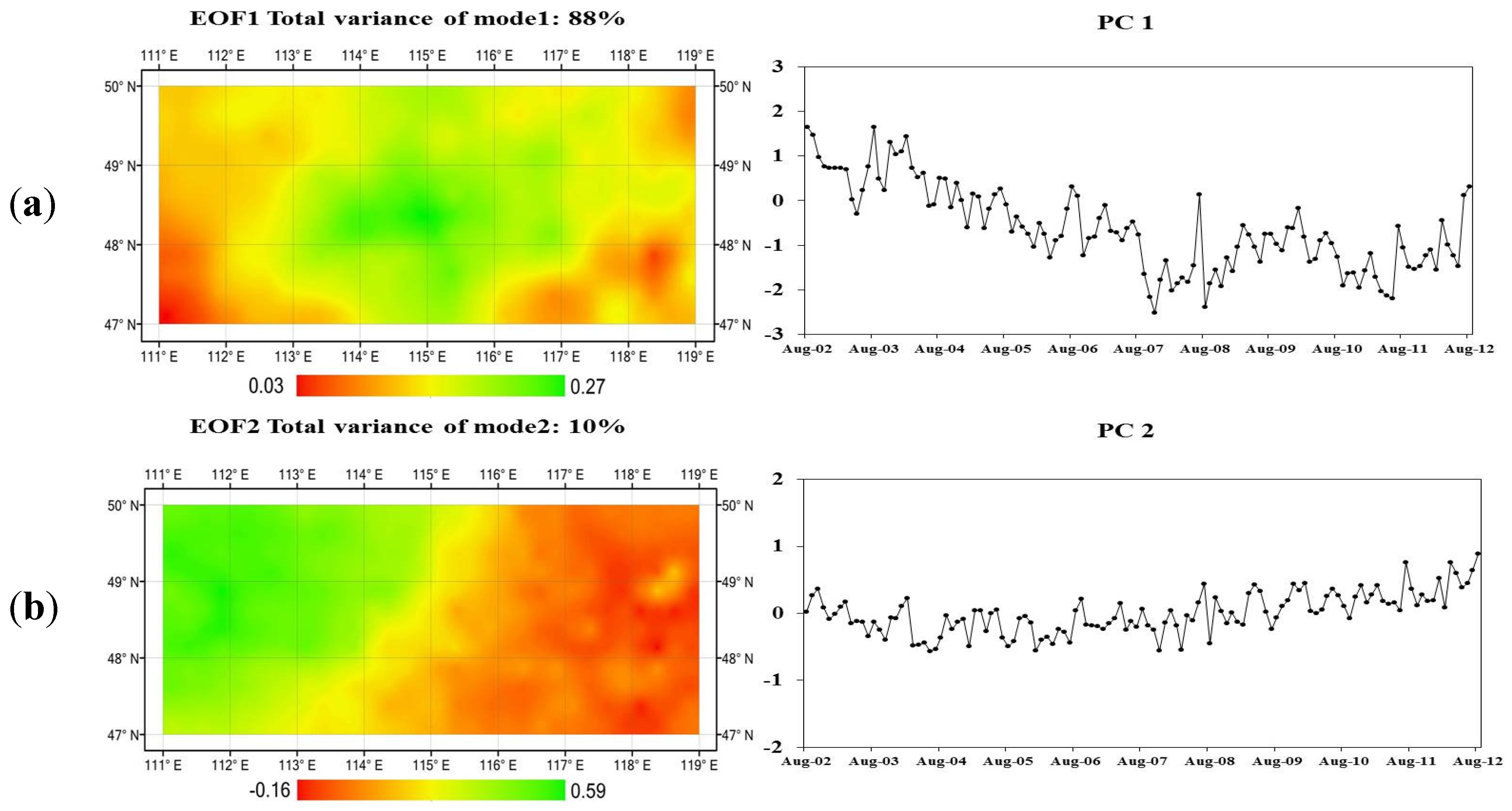
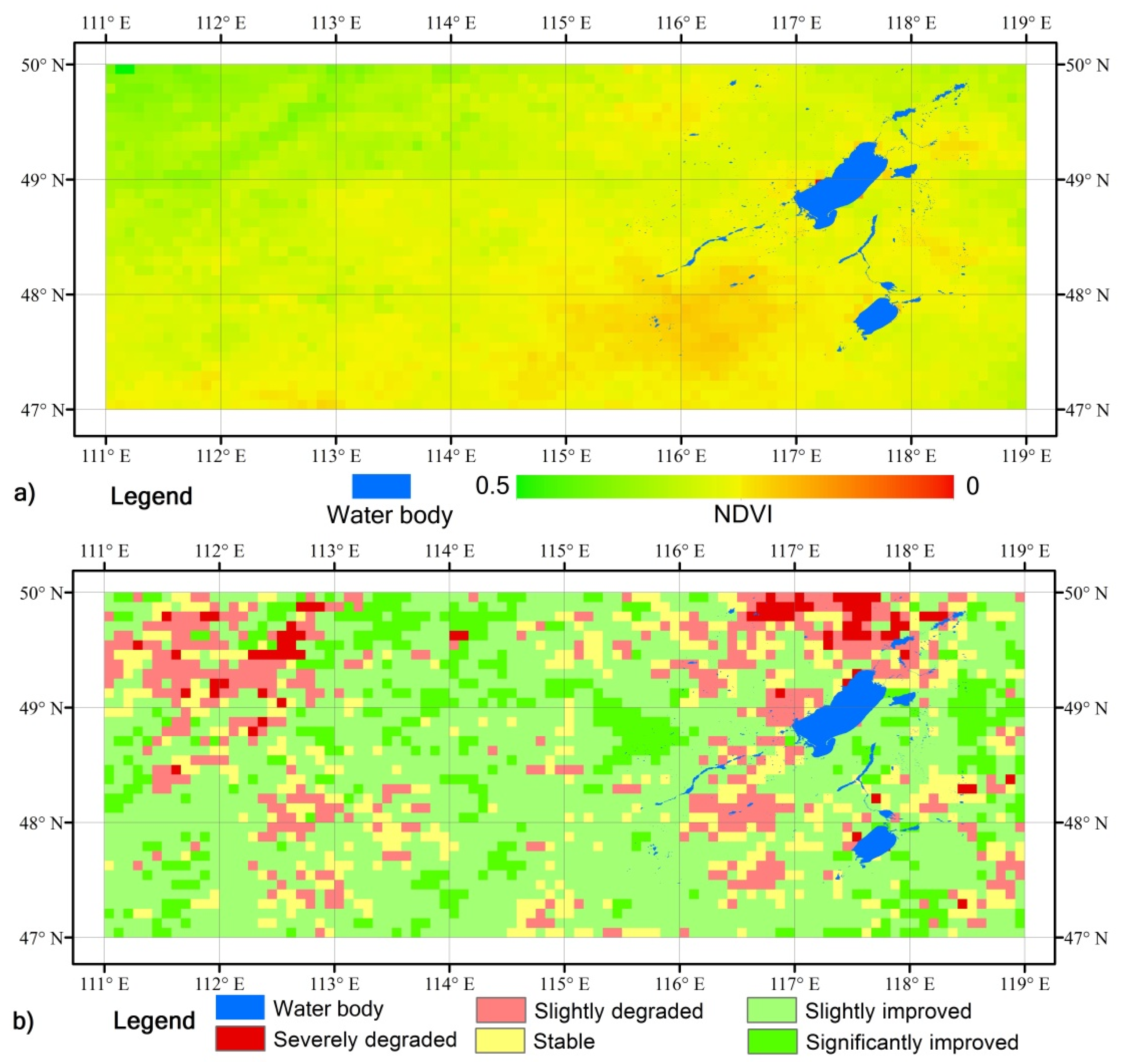
5.4. Vegetation Response to Water Resource Change

| TSNDVI | Z | NDVI Trend | Area (%) |
|---|---|---|---|
| <−0.0005 | <−1.96 | Severely degraded | 2.69% |
| <−0.0005 | −1.96–1.96 | Slightly degraded | 13.80% |
| −0.0005–0.0005 | −1.96–1.96 | Stable | 13.51% |
| ≥0.005 | −1.96–1.96 | Slightly improved | 57.35% |
| ≥0.005 | ≥1.96 | Improved | 12.64% |
6. Conclusions
Acknowledgments
Author Contributions
Conflicts of interest
References
- Long, D.; Scanlon, B.R.; Longuevergne, L.; Sun, A.-Y.; Fernando, D.N.; Save, H. GRACE satellites monitor large depletion in water storage in response to the 2011 drought in Texas. Geophys. Res. Lett. 2013, 40, 3395–3401. [Google Scholar] [CrossRef] [Green Version]
- Huffman, G.J.; Bolvin, D.T.; Nelkin, E.J.; Wolff, D.B.; Adler, R.F.; Gu, G.; Yang, H.; Kenneth, P.B.; Erich, F.; Stocker, E.F. The TRMM multi-satellite precipitation analysis (TMPA): Quasi-global, multiyear, combined-sensor precipitation estimates at fine scales. J. Hydrometeorol. 2007, 8, 38–55. [Google Scholar] [CrossRef]
- Wang, X.; Gong, P.; Zhao, Y.; Xu, Y.; Cheng, X.; Niu, Z.; Luo, Z.; Huang, H.; Sun, F.; Li, X. Water-level changes in China’s large lakes determined from ICESat/GLAS data. Remote Sens. Environ. 2013, 32, 131–144. [Google Scholar] [CrossRef]
- Gokmen, M.; Vekerdy, Z.; Verhoef, W.; Batelaan, O. Satellite based analysis of recent trends in the ecohydrology of a semi-arid region. Hydrol. Earth Syst. Sci. Discuss. 2013, 10, 6193–6235. [Google Scholar] [CrossRef]
- Zhang, X.; Zwiers, F.W.; Hegerl, G.C.; Lambert, F.H.; Gillett, N.P.; Solomon, S.; Nozawa, T. Detection of human influence on twentieth-century precipitation trends. Nature 2007, 448, 461–465. [Google Scholar] [CrossRef] [PubMed]
- Syed, T.H.; Famiglietti, J.S.; Rodell, M.; Chen, J.; Wilson, C.R. Analysis of terrestrial water storage changes from GRACE and GLDAS. Water Resour. Res. 2008, 44. [Google Scholar] [CrossRef]
- Fensholt, R.; Rasmussen, K. Analysis of trends in the Sahelian “rain-use efficiency” using GIMMS NDVI, RFE and GPCP rainfall data. Remote Sens. Environ. 2011, 115, 438–451. [Google Scholar] [CrossRef]
- Du, J.; He, F.; Zhang, Z.; Shi, P. Precipitation change and human impacts on hydrologic variables in Zhengshui River Basin, China. Stoch. Environ. Res. Risk Assess. 2011, 25, 1013–1025. [Google Scholar] [CrossRef]
- Moiwo, J.P.; Tao, F.; Lu, W. Analysis of satellite-based and in situ hydro-climatic data depicts water storage depletion in North China Region. Hydrol. Process. 2012, 27, 1110–1020. [Google Scholar]
- Dorothea, D.; Richard, G. Remote sensing analysis of lake dynamics in semi-arid regions: Implication for water resource management. Water 2013, 5, 698–727. [Google Scholar] [CrossRef]
- Duan, Z.; Bastiaanssen, W.G.M. Estimating water volume variations in lakes and reservoirs from four operational satellite altimetry databases and satellite imagery data. Remote Sens. Environ. 2013, 134, 403–416. [Google Scholar] [CrossRef]
- Eckert, S.; Hüsler, F.; Liniger, H.; Hodel, E. Trend analysis of MODIS NDVI time series for detecting land degradation and regeneration in Mongolia. J. Arid Environ. 2015, 113, 16–28. [Google Scholar] [CrossRef]
- Jiang, W.; Yuan, L.; Wang, W.; Cao, R.; Zhang, Y.; Shen, W. Spatio-temporal analysis of vegetation variation in the Yellow River Basin. Ecol. Indic. 2015, 51, 117–126. [Google Scholar] [CrossRef]
- Shinoda, M.; Nachinshonhor, G.U.; Nemoto, M. Impact of drought on vegetation dynamics of the Mongolian steppe: A field experiment. J. Arid Environ. 2010, 74, 63–69. [Google Scholar] [CrossRef]
- Da Silva, E.C.; de Albuquerque, M.B.; de Azevedo Neto, A.D.; da Silva Junior, C.D. Drought and its consequences to plants—From individual to ecosystem. In Responses of Organisms to Water Stress; InTech: Rijeka, Croatia, 2013. [Google Scholar]
- Kummerow, C.; Barnes, W.; Kozu, T.; Shiue, J.; Simpson, J. The tropical rainfall measuring mission (TRMM) sensor package. J. Atmos. Ocean. Technol. 1998, 15, 809–817. [Google Scholar] [CrossRef]
- Yatagai, A.; Xie, P.; Kitoh, A. Utilization of a new gauge-based daily precipitation dataset over monsoon Asia for validation of the daily precipitation climatology simulated by the MRI/JMA 20-km-mesh AGCM. SOLA 2005, 1, 193–196. [Google Scholar] [CrossRef]
- Chen, Y.; Velicogna, I.; Famiglietti, J.S.; Randerson, J.T. Satellite observations of terrestrial water storage provide early warning information about drought and fire season severity in the Amazon. J. Geophys. Res. Biogeosci. 2013, 118, 495–504. [Google Scholar] [CrossRef]
- Fan, Y.; van den Dool, H. A global monthly land surface air temperature analysis for 1948–present. J. Geophys. Res. 2008, 113. [Google Scholar] [CrossRef]
- LEGOS/GOHS. Available: http://www.legos.obs-mip.fr (accessed on 3 January 2013).
- U.S. Government Computer. Available online: http://e4ftl01.cr.usgs.gov/MOLT/MOD09A1 (accessed on 14 March 2015).
- Landsat Data Access. Available online: http://landsat.usgs.gov/Landsat_Search_and_Download.php (accessed on 20 March 2015).
- Center for Space Research. Available online: ftp://podaac.jpl.nasa.gov/allData/grace/L2/CSR/RL05/ (accessed on 12 February 2013).
- Swenson, S.; Chambers, D.; Wahr, J. Estimating geocenter variations from a combination of GRACE and ocean model output. J. Geophys. Res. 2008, 113. [Google Scholar] [CrossRef]
- Duan, X.J.; Guo, J.Y.; Shum, C.K.; Wal, W. On the postprocessing removal of correlated errors in GRACE temporal gravity field solutions. J. Geod. 2009, 83, 1095–1106. [Google Scholar] [CrossRef]
- Zhang, Z.-Z.; Chao, B.F.; Lu, Y.; Hsu, H.-T. An effective filtering for GRACE time-variable gravity: Fan filter. Geophys. Res. Lett. 2009, 36. [Google Scholar] [CrossRef]
- GIMMS, “ECOCAST”, NASA. Available online: http://ecocast.arc.nasa.gov/data/pub/gimms/ (accessed on 19 April 2015).
- Longuevergne, L.; Florsch, N.; Elsass, P. Extracting coherent regional information from local measurements with Karhunen-Loève transform: Case study of an alluvial aquifer (Rhine valley, France and Germany). Water Resour. Res. 2007, 43. [Google Scholar] [CrossRef] [Green Version]
- Perry, M.A.; Niemann, J.D. Analysis and estimation of soil moisture at the catchment scale using EOFs. J. Hydrol. 2007, 334, 388–404. [Google Scholar] [CrossRef]
- Song, X.; Duan, Z.; Jiang, X. Comparison of artificial neural networks and support vector machine classifiers for land cover classification in Northern China using a SPOT-5 HRG image. Int. J. Remote Sens. 2012, 33, 3301–3320. [Google Scholar] [CrossRef]
- Xu, H. Modification of normalised difference water index (NDWI) to enhance open water features in remotely sensed imagery. Int. J. Remote Sens. 2006, 27, 3025–3033. [Google Scholar] [CrossRef]
- Deus, D.; Gloaguen, R. Remote Sensing Analysis of Lake Dynamics in Semi-Arid Regions: Implication for Water Resource Management, Lake Manyara, East African Rift, Northern Tanzania. Water 2013, 5, 698–727. [Google Scholar] [CrossRef]
- Cai, B.F.; Yu, R. Advance and evaluation in the long time series vegetation trends research based on remote sensing. J. Remote Sens. 2009, 13, 1170–1186. [Google Scholar]
- Hoaglin, D.C.; Mosteller, F.; Tukey, J.W. Understanding Robust and Exploratory Data Analysis; Wiley: New York, NY, USA, 1983. [Google Scholar]
- National Center for Agricultural Scientific Data Sharing. Available online: http://grassland.agridata.cn/client.c?method=fgbz&menuid=106&id=59 (accessed on 26 May 2015).
- Ding, M.; Zhang, Y.; Liu, L.; Zhang, W.; Wang, Z.; Bai, W. The relationship between NDVI and precipitation on the Tibetan Plateau. J. Geogr. Sci. 2007, 17, 259–268. [Google Scholar] [CrossRef]
© 2015 by the authors; licensee MDPI, Basel, Switzerland. This article is an open access article distributed under the terms and conditions of the Creative Commons Attribution license (http://creativecommons.org/licenses/by/4.0/).
Share and Cite
Ning, S.; Ishidaira, H.; Udmale, P.; Ichikawa, Y. Remote Sensing Based Analysis of Recent Variations in Water Resources and Vegetation of a Semi-Arid Region. Water 2015, 7, 6039-6055. https://doi.org/10.3390/w7116039
Ning S, Ishidaira H, Udmale P, Ichikawa Y. Remote Sensing Based Analysis of Recent Variations in Water Resources and Vegetation of a Semi-Arid Region. Water. 2015; 7(11):6039-6055. https://doi.org/10.3390/w7116039
Chicago/Turabian StyleNing, Shaowei, Hiroshi Ishidaira, Parmeshwar Udmale, and Yutaka Ichikawa. 2015. "Remote Sensing Based Analysis of Recent Variations in Water Resources and Vegetation of a Semi-Arid Region" Water 7, no. 11: 6039-6055. https://doi.org/10.3390/w7116039