A Dynamic, Multivariate Sustainability Measure for Robust Analysis of Water Management under Climate and Demand Uncertainty in an Arid Environment

Abstract

Considering water resource scarcity and uncertainty in climate and demand futures, decision-makers require techniques for sustainability analysis in resource management. Through unclear definitions of “sustainability”, however, traditional indices for resource evaluation propose options of limited flexibility by adopting static climate and demand scenarios, limiting analysis variables to a particular water-use group and time. This work proposes a robust, multivariate, dynamic sustainability evaluation technique and corresponding performance indicator called Measure of Sustainability (MoS) for resource management that is more adapted to withstand future parameter variation. The range of potential future climate and demand scenarios is simulated through a calibrated hydrological model of Copiapó, Chile, a case study example of an arid watershed under extreme natural and anthropogenic water stresses. Comparing MoS and cost rankings of proposed water management schemes, this paper determines that the traditional evaluation method not only underestimates future water deficits, but also espouses solutions without considering uncertainties in supply and demand. Given the uncertainty of the future and the dependence of resources upon climate and market trajectories, the MoS methodology proposes solutions that, while perhaps are not the most optimal, are robust to variations in future parameter values and are thus the best water management options in a stochastic natural world.

1. Introduction

In the 20th century, the world population has tripled, but water use has increased six-fold, indicating augmented stresses on limited resources [1]. In light of this, politicians and decision-makers seek solutions to meet demand [2]. One approach is a shift to include both supply and demand management through Integrated Water Resources Management (IWRM) (e.g., [3,4,5,6,7,8,9]). Of growing importance in IWRM, one such method has been to improve resource efficiency through watershed-scale application of water reuse and recycling (WRR) technologies [10,11,12].

Equitable water use as proposed by IWRM faces challenges due to continuous structural transformations in society and the environment [13], yielding problems of high complexity and uncertainty [14,15,16]. Climate change will lead to uncertain future water supplies [17], while population growth, technological innovation, composition of future economies, and dynamic stakeholder goals add further demand-side uncertainties [18]. As such, methodological tools are required that enable the assessment of sustainability under an uncertain future.

It is well known, however, that defining sustainability in a rigorous and meaningful manner is challenging at best [19,20]. The first widely accepted articulation of the term sustainable development, published in the Brundtland report, calls for a “development that meets the needs of the present without compromising the ability of future generations to meet their own needs” [21]. Since its publication, close to 300 other attempts at a definition of “sustainability” have been published (e.g., [19,22,23,24]), none of which is universally accepted, but there is increasing consensus that discussions thereof should include uncertainty [25]. Under uncertainty, we must seek solutions that may not be the most optimal under present conditions, but are the most robust (i.e., less likely to fail and more immune to the effects of failure due to factors of uncertainty) [26,27]. We argue that any robust measure of water resources sustainability must consider three major sources of uncertainty under a decision support analysis as represented by the following questions [20,22]: (1) for whom is the resource being sustained; (2) at what time will sustainability be determined; (3) under what future conditions will the resources remain sustainable. From hereafter the sources of uncertainty associated with these questions will be respectively referred as to Whomever, Whenever, and No Matter What.

In line with this, for over three decades there have been attempts to create water risk indices, easy for lay-users to understand but capable of merging the intricacies of resource scarcity into a single unified number, a “synthesis of numerous factors into one given factor” [28]. Decision support tools in water resource management often aim to do this (e.g., [29,30,31,32,33,34,35]). For example, to quantify risk in a reservoir to optimize water management under uncertainty and scarcity, Hashimoto et al. proposed a landmark methodology, called RRV, that quantifies risk in terms of the frequency (Reliability, R), duration (Resilience, R), and magnitude (Vulnerability, V) of system failure [29]. RRV has been applied in numerous hydrologic settings to quantify water quantity and quality risk under varying scenarios (i.e., [13,36,37]). Loucks [31] and Sandoval-Solis et al. [35] unified the RRV factors, proposing multi-criteria analysis methodologies that consider not only the needs of various stakeholders but also incorporate multiple risk measures.

These methodologies, however, are similar to traditional analyses techniques in that, while addressing the first two sources of resource uncertainty (Whomever and Whenever) through dynamic multi-criteria analysis, their simplification of variable trajectories overlooks the resources’ supply and demand futures (No Matter What). By assuming unchanging climate parameters and resource use, these previous studies are susceptible to adopting solutions that, while optimal for present conditions, are incapable of responding to variations in these. Overlooking uncertainty in future conditions risks the possibility of espousing solutions unsustainable in the very future for which they are proposed.

The objective of this study is to propose a methodology that encompasses multiple sources of uncertainty in decision-making, including climate change, population growth, and demand trajectories defined by future socio-economic scenarios. While traditional engineering solutions operating under deterministic parameters often invoke “optimization” as the problem-solving goal, in stochastic or uncertain situations “robustness” must serve as the objective so as to maintain performance of the system when subjected to unpredictable perturbations [38]. By evaluating the performance of a dynamic and multivariate risk index in response to the range of potential supply and demand futures, this methodology seeks robust sustainable options under future uncertainties [39]. In our approach, we incorporate climate change projections, based on downscaled Global Climate Projections (GCP) following Special Report on Emission scenarios (SRES) and Representative Concentration Pathway (RCP) scenarios, as well as growth projections provided by experts in each water sector, considering conservative, average, and extreme demand scenarios. These are integrated into a Water Evaluation And Planning (WEAP)-MODFLOW coupled hydrology model that simulates the surface-subsurface system. To assess future outcomes we propose a new dynamic multidimensional evaluation methodology for sustainable water management plan ranking and selection.

This new methodology for robust sustainability analysis is presented in Section 2 of this paper, and in Section 3 is applied to the Copiapó River basin in Chile, one of the most arid regions in the world in which strong economic and population growth is taking place due to agricultural and mining industries. A recent study of this site [40] explored several water management strategies, calling for a reduction in demand of 20%–30%, a range achievable in practice through effective WRR [41]. This study, while providing useful planning information, adopted the oversimplifying assumptions common to current water management analyses of constant supply and demand futures, single variable analysis, and static rather than dynamic evaluation of sustainability (e.g., [42,43,44]). Results from the application of our new dynamic, multivariate, robust sustainability measure are compared in Section 4 with those using a static, single-variable, deterministic future (i.e., [40]) to demonstrate the importance of considering these often overlooked factors in resource decision-making. Finally, Section 5 presents the main conclusions of this work.

2. Materials and Methods

2.1. Previous Sustainability Methods—RRV and Sustainability Index

Previous studies have made important contributions to the field of sustainability analysis. Recognizing the dynamic nature of risk related to water resource management, Hashimoto et al. developed the RRV (Reliability, Resiliency, Vulnerability) methodology [29]. Reliability describes the probability a system is in a satisfactory state, resiliency is a measure of how quickly a system recovers from failure, and vulnerability is the expected magnitude of failure. For application in IWRM, consider two time series of water demand X_D(t) and supply X_S(t), which can be broken into n equal time increments (t = 1,2,..,n). We define a water deficit during an interval t, as $D_t=(X_{D,t}-X_{S,t})H(X_{D,t}-X_{S,t})$, where $X$ represents amount of water and $H\left(x\right)$ is the Heaviside step function, which assigns a value of $D_t=0$ when supply exceeds demand, which we say represents a satisfactory state (S). Likewise, a state of failure (F) is defined as when demand exceeds supply, that is $X_{D,t}> X_{S,t}$ or D_t > 0 = $(X_{D,t}-X_{S,t})$. RRV for a certain variable i, where N° represents the number of occurrences, are given by:

$$Reliabilit{y}^i={\text{α}}^i=P\left[X_t\in S\right]=\frac{N^o\left(D_t=0\right)}{n}$$

(1)

$$Resilienc{e}^i={\rho }^i=P\left\{X_t\in S,X_{t-1}\in F\right\}=\frac{\left\{N^o\left(D_t=0\right)\text{|}{D}_{t-1}>0\right\} }{N^o\left(D_t>0\right)}$$

(2)

$$Vulnerabilit{y}^i={\text{ε}}^i=E\left[X_t|X_t\in F\right]=\frac{{{\displaystyle \sum }}_{t=0}^{t=n}{D}_t}{N^o\left(D_t>0\right)}$$

(3)

While these three metrics are individually informative, Loucks [31,45] proposed combining the RRV measures in such a way as to define a sustainability index (SI). In particular he proposed the following index $S{I}_L$, given by:

$$S{I_L}^i={\text{α}}^i{\rho }^i\left(1-{\text{ε}}_{rel}^i\right)$$

(4)

Note that $S{I}_L$ includes the concept of relative vulnerability, ${\epsilon }_{rel}$, which corresponds to a normalized measured of the maximum vulnerability within the context of all the management alternatives being compared for sustainability:

$${\text{ε}}_{rel}^i={\text{ε}}^i/\left(Ma{x}^{All}\text{ε}\right)$$

(5)

$S{I}_L$ allows for the comparison of relative sustainability between competing management options, simplifying it down to a single number for ease of use by water resource managers [46,47]. Indeed, $S{I}_L$ summarizes the performance of alternative policies from the perspective of water users and the environment, and it is also a measure of a system’s adaptive capacity to reduce its vulnerability [35]. It ranges from 0 to 1 with 1 indicating complete sustainability. If any one measure has a value of 0, the sustainability will also be 0 (i.e., no complete tradeoff is possible) and its multiplicative form implicitly weighs heavily the worst performing criteria.

Sandoval-Solis et al. [35] suggest improving the original index in structure, scale, and content to make it more flexible and adjustable to the requirements of each basin. Thus, they add two new dimensionless resource performance criteria to Louck’s original SI, which are integral to resource planning: standard deviation (σ, Equation (6)), a measure of variability, and maximum deficit (Equation (7)), a measure of worst-case scenario:

$${\text{σ}}^i=\frac{\sqrt{\left[{{\displaystyle \sum }}_{t=1}^{t=n}{\left(X_{S,t}^i-{\overline{X}}_S^i\right)}^2\right]/\left(n-1\right)}}{X_{D,t}^i}$$

(6)

$${\text{δ}}_m=\frac{max\left(D_{Annual}^i\right)}{X_{D,t}^i}$$

(7)

Moreover, Sandoval-Solis et al. [35] offer a generalized form of the SI calculation, allowing for the inclusion of other criteria depending upon the user’s perception of the necessities of each case:

$$S{I}^i={\left[{\displaystyle \prod }_{m=1}^M{C}_m^i\right]}^{\raisebox{1ex}{$1$}\!\left/ \!\raisebox{-1ex}{$M$}\right.}$$

(8)

where $S{I}^i$ is the sustainability index for variable i, calculated using M performance criteria $C_m^i$. This approach solves a problem of results scaling, as the geometric average of the criteria values still penalizes poor performance, but is more representative (e.g., three criteria values of 50% each would have a logical 50% final rating using Sandoval-Solis, compared to a 12.5% using Loucks).

As might be seen in the above equations, RRV analysis (and thus the SI as well) meets the uncertainty criteria of Whenever, using dynamic rather than static performance measures independent of when they are evaluated in the delimited time frame n. Also, the index may be calculated for more than one watershed variable so as to include SI calculations for a range of variables from various stakeholder sectors, thus meeting the uncertainty criteria of Whoever stated above as well. Indeed, we initially propose to consider the agriculture, industry, and potable water production sectors, although other stakeholder groups of relevance for the watershed under study may also be considered. However, the third sustainability criterion (i.e., No Matter What), which deals with uncertainty in future variable values, has been largely overlooked (No Matter What). To meet this criterion, climate change and future demand scenarios caused by uncertainties of markets, values, and population must be included. Overall, decision-makers wish to select the management option that, although possibly not optimal, is robust to uncertain future variables and thus able to withstand the unforeseen [20].

2.2. Proposed Sustainability Methodology—Measure of Sustainability (MoS)

We propose a sustainability measure that continues to address the first two uncertainty questions, maintaining the multisectorial approach proposed by Loucks to address the environmental, political, social, and economic impacts of water resources [31]. In addition, we retain the five-factor RRV sustainability index presented by Sandoval-Solis et al. [35], but this research advances the state of present sustainability evaluation in that it addresses uncertainty in future parameters under which decisions will be forced to operate. By considering a range of possible supply futures, and using climate change models as well as a cone of potential demand trajectories, this research proposes a robust methodology for water management decision-making. To differentiate from previous indices, we shall refer to this method as the Measure of Sustainability (MoS).

2.2.1. Future Water Demand

Given growth observed in recent years not only in population but in per capita consumption and in economies, static projections can be both erroneous and lead to inadequate long-term planning. While future conditions might experience a wide range of potential trajectories, econometrics in resource planning and sociological literature lead us to consider the three different logical growth options presented in Table 1 to estimate the population in year t, P_t, given the initial population in the reference year 0, P₀. Throughout its life cycle, any socio-economic sector may experience all three of these different growth patterns [48]. During the early stages of sectorial growth, rapid change is modeled according to a uniform percentage growth rate r (exponential/extreme growth). Later, this rate steadies to a constant K (linear/average growth). Finally, as the sector nears its saturation level, the rate of growth continues to decrease with limit at 0 (cubic/conservative growth). Given the difficulty of determining in which of these three stages present conditions lie, we consider all three possibilities simultaneously through a “demand cone” (Figure 1) which, starting with present values, expands into the future to consider the range of possibilities. Demand futures in potable, agricultural, and industrial/mining water will be considered separately, each using all three of the demand cone possible scenarios: extreme, average, and conservative growth (Figure 1, Table 1) [49,50].

Table 1. Generic future demand models according to life cycle stage.

Life Cycle Stage	Growth Scenario	Model	Equation
Early	Extreme (Ext)	Exponential	$P_t=P_0{e}^{rt}$
Middle	Average (Avg)	Linear	$P_t=P_0+Kt$
Late	Conservative (Con)	Declining Growth	$P_t=P_0+{\text{α}}_3{t}^3+{\text{α}}_2{t}^2+{\text{α}}_{1}t$

Table 1. Generic future demand models according to life cycle stage.

Life Cycle Stage	Growth Scenario	Model	Equation
Early	Extreme (Ext)	Exponential	$P_t=P_0{e}^{rt}$
Middle	Average (Avg)	Linear	$P_t=P_0+Kt$
Late	Conservative (Con)	Declining Growth	$P_t=P_0+{\text{α}}_3{t}^3+{\text{α}}_2{t}^2+{\text{α}}_{1}t$

Figure 1. Generic “demand cone” of future trajectories; extreme (Ext), average (Avg), and conservative (Cons) futures.

Figure 1. Generic “demand cone” of future trajectories; extreme (Ext), average (Avg), and conservative (Cons) futures.

2.2.2. Future Climates

Future supply variation must also be considered in the analysis, as it might provide an even greater source of uncertainty. Both Loucks [31] and Sandoval-Solis et al. [35] recognize the need for a sustainability analysis that encompasses climate change (e.g., [51]), but neither attempts it. Given documented potential changes in global and regional climate patterns that affect both temperature and precipitation distribution, it is crucial for resource planning to consider climate change.

Given the large grid size (over 1° in latitude and longitude) of current GCP´s compared with watershed scales, GCM projections must be downscaled for use in hydrologic supply analysis. For smaller watersheds such as that of Copiapó, Chile, a single-climate model grid cell might be larger than an entire watershed, covering elevations between 0 and 6000 m, with average annual precipitations ranging from 0 to 500 mm. Thus, the predictions of the climate models must be adjusted so as to be applied to discrete weather stations located within the watershed. Following the quantile mapping and bias correction methodology of Wood et al. [52] that is used by Meza et al. [53], the downscaling process adopted in this study first attempts to correct for a spatial bias, using the inverse distance squared method [54] between the four grid points nearest the water station of interest to determine a geometric average. Then, comparing the probability distribution of the model average for the control period (2000–2010) with the probability distribution of historical data, the methodology adjusts for elevation and seasonal biases by shifting the Probability Distribution Function (PDF) of the model vertically and stretching horizontally to align with the mean and standard deviation of the historical data. This same shift, then, is applied to the climate projection data for future temperature and precipitation. While this methodology does assume that the bias between the historical and control data shall remain constant in the future, the factors causing the bias (location, elevation, seasons) typically change slowly enough not to be a concern [52].

Dozens of climate models exist, which in turn consider different emissions scenarios, resulting in hundreds of potential hydrologic supply futures. Users of this methodology must first select a period for evaluation; we have chosen 30 years as a typical period of capital investment. Calculating the 30-year changes in average annual temperature ($\Delta T$, in °C) and annual precipitation ($\Delta P$, in %) for different climate models under a variety of emission scenarios for the watershed, results are plotted as may be observed in Figure 2. Given that we are not specifically interested in the performance of the system under each and every climate model (blue points, Figure 2), but rather in the range of possible futures, we choose to limit the volume of data by selecting the four extreme climate models (dry-hot, dry-cool, wet-hot, wet-cool) as well as an average model to represent the variety of possible climates (red points, Figure 2). The dotted vertical line in Figure 2 represents 2.5 standard deviations above the mean for percent change in precipitation. While we have chosen to exclude outliers that fall to the right of this line (p = 0.006), this determination is made by the user of the methodology. Indeed, the election of the four extreme climate scenarios is subjective, and if desired, confidence intervals could be used depending on the decision-maker’s perspective. For the final MoS calculation, results for these five models $X_i=\left(X_{i,P},X_{i,T}\right)$ will be weighted based upon the percentage of all climate models $M_j=\left(M_{j,P},M_{j,T}\right)$ closest to each on the $\Delta T vs. \Delta P$ plot (e.g., Figure 2 below for the Copiapó, Chile example). For each climate model $M_j$, Euclidean distances are calculated between the model and each of the five representative models $X_i$. The model $M_j$ will be represented by the closest $X_i$.

Figure 2. Shown is $\Delta T vs. \Delta P$, 30-year average percent change in climate (Copiapó, Chile example). Blue points indicate all climate models with emission scenarios while red points are the chosen representative scenarios. Vertical dotted line indicates cut-off for outliers (>2.5 standard deviations above mean).

Figure 2. Shown is $\Delta T vs. \Delta P$, 30-year average percent change in climate (Copiapó, Chile example). Blue points indicate all climate models with emission scenarios while red points are the chosen representative scenarios. Vertical dotted line indicates cut-off for outliers (>2.5 standard deviations above mean).

2.2.3. Computation of the MoS Index

For robust analysis that addresses the three previously mentioned major questions of uncertainty, each management plan is evaluated using the RRV-based five-factor SI presented by Sandoval-Solis et al. [35] (Equation (9)) for the four different water use dimensions (environmental, economic, social, political) under five different climate models and three different demand permutations, yielding one final MoS score (Figure 3).

Following is a list of generalized steps for the calculation of the MoS, applicable to any study site (Figure 3):

• Identify the five climate models and three demand trajectories using the process described above for a total of 15 combinations of potential futures;
• For each of these 15 futures, collect time-series data for variables representing the four water use dimensions (environmental, political, social, economic), giving 60 variables to be considered over a predetermined time frame;
• For each of these 60 variables i, calculate sustainability according to:

  $$S_{SS}^i={\left[{\alpha }^i{\rho }^i\left(1-{\epsilon }_{rel}^i\right)\left(1-{\delta }_M^i\right)\left(1-{\sigma }^i\right)\right]}^{1/5}$$

  (9)
• For each potential future, combine the $S{I}_{SS}^i$ scores for the four water use dimensions through a weighted sum by means of user-defined weights of importance to give a future demand score (default: equal importance [31]);
• For each climate model, combine the future demand scores from Step 4 for each of the three demand trajectories by using user-defined weights of potentiality (default: equally probable) (red diamond in Figure 3);
• Calculate the final index score (MoS) by combining the five $S{I}_{SS}^i$ scores from Step 5, weighted according to the method described in the previous section, based on the percentage of all climate models closet to each simulated future on the $\Delta T vs. \Delta P$graph. (Figure 2).

Figure 3. Flow chart of Steps 1–5 of MoS methodology for Avg. climate scenario. Step 6 combines all climate scenarios using weights from $\Delta T vs. \Delta P$ plot for final MoS score. Step numbers correspond to the list of steps outlined below.

Figure 3. Flow chart of Steps 1–5 of MoS methodology for Avg. climate scenario. Step 6 combines all climate scenarios using weights from $\Delta T vs. \Delta P$ plot for final MoS score. Step numbers correspond to the list of steps outlined below.

To measure performance in the water use dimensions mentioned in Step 2 of the MoS methodology above, decision-makers may select any dynamic variable represented by a time-series that they feel exemplifies the state of water in relation to the dimension. This paper, however, proposes the variables observed in Table 2, with their respective failure thresholds, as simple but succinct measures of water dimension “health”. The economic dimension will be gauged by the sum of the percentage of water demand met for each productive stakeholder, weighted by that member’s percent participation in the watershed economy. Economic failure shall be considered below 100% of weighted water demand, as healthy economies generally do not allow for deflation. Given the crucial importance of domestic potable water for health, comfort, and hygiene, the threshold for the social variable of the percentage of potable water demand met will be set at 100%; this threshold is a metric common to studies of potable water supply [55]. The political impact of water shall be considered in a state of failure when less than 75% of stakeholders have their water rights met. With more than 25% of water rights left unsatisfied, growing discontent among voters begins to make political re-election more difficult for a single decision-maker in a democratic watershed (inclusion threshold of competitor) [56].

Table 2. Sustainability variables and failure thresholds for water use dimensions.

Water Use Dimension	Variable	Failure Threshold
Environmental	Aquifer level	Slope (current-critical)
Economic	% demand economic weight	Less than 100%
Social	% of potable demand met	Less than 100%
Political	% of all demands met	Less than 75%

Table 2. Sustainability variables and failure thresholds for water use dimensions.

Water Use Dimension	Variable	Failure Threshold
Environmental	Aquifer level	Slope (current-critical)
Economic	% demand economic weight	Less than 100%
Social	% of potable demand met	Less than 100%
Political	% of all demands met	Less than 75%

Special mention must be made for the environmental water variable, aquifer volume. While the other water use dimensions are evaluated according to variations on demand met, and thus not dependent on whether a zone is arid or not, the variable chosen to evaluate the environmental dimension (aquifer volume) is particular to arid basins. In more water-rich environments, a suitable variable to measure the health of the environmental dimension might be stage height of a river or total volume of a reservoir; such measures, however, are often not appropriate for arid zone hydrology. In these areas, groundwater often provides a large proportion of the resource and thus aquifer volume serves as a reasonable evaluation variable. Nevertheless, the general methodology proposed would be equally applicable under more humid scenarios given appropriately defined evaluation variables.

For arid basins, while a certain depth to groundwater could be set as the failure threshold, due to overuse of groundwater compared with the relatively slow recharge process in water-scarce zones, true sustainable use of these resources (that is, maintaining resources as constant) is quite simply not feasible. Recovery once surpassing a static threshold of depth, will most likely not occur unless demand is reduced by unmanageable amounts. “Sustainability” in this case shall be defined as the continual presence of water resources during the modeled time period in more than half of the current wells in the watershed. Using the example of Copiapó (Chile) presented later, this threshold shall be surpassed when the aquifer level falls more than 60 m below the land surface, or rather when the total volume drops below 7373 million m³. In some sense this approach defines sustainability as maintaining a sufficiently slow decline in resources with respect to time, in the hope that over several decades alternative unidentified solutions will emerge that can address declining resources effectively. While optimistic, it is likely the only currently realistic option. Thus, for similar cases in arid regions where withdrawal greatly exceeds recharge, the environmental dimension shall be evaluated according to a sloping linear threshold between present volume levels and the critical volume expected at the end of the simulation period (i.e., a slope of −42.54 million m³/year for the Copiapó case study to be illustrated below). While the relative variables and failure thresholds for these four water use dimensions are all interchangeable according to the values and opinion of the decision-maker, we believe that these proposed variables and failure thresholds represent the logical functioning of a sustainable watershed.

3. Application to a Case Study

To demonstrate the application of this generalized methodology for a robust, dynamic, multi-criteria sustainability index, we utilize the example of the Copiapó River Basin (18,538 km²), located in the Atacama Desert of Chile (Figure 4, divided into six administrative sectors) and whose main urban center is the city of Copiapó (elev. 391 m, pop. 158,000, sector 4a). This snowmelt-dominated watershed, situated between 27° S and 29º S latitude, represents a basin under extreme water stress. Positioned in an arid region (28 mm average annual precipitation over the entire watershed, but with large inter-annual variation due to El Niño and large spatial variation due to elevation change) in which constantly growing demands increasingly strain scarce water resources, the Copiapó River Basin experiences an overexploitation of water resources by 30%–40%. Mining, agriculture, water utility, and tourism all compete for access to limited resources; indeed, water rights already granted are estimated to represent almost 500% of the groundwater recharge rate. The mining sector (copper, gold, iron) owns 17% of these rights while the agricultural sector holds 56% (mostly grapes, olives, and vegetable crops) [40]. The recent gifting of extraction rights by the Candelaria mine to the Colla indigenous community has skewed these percentages even further towards agriculture [57]. Growth in both activities, however, is considered fundamental to regional and national economic development with 33 new mining projects (est. $50 billion USD), and a 20% increase in agricultural surface area projected over the next five years [58]. Additionally, economic development has led to an increase of local potable consumption (8.8% of water rights) [40]. This water stress has left the Lautaro Reservoir empty during most months and is forcing decision-makers to look elsewhere for solutions. Further physical and operational details of the Copiapó watershed may be found in Suarez et al. [40].

Figure 4. The Copiapó River, with an average flow of ~1.5 m³/s, largely from snowmelt, drops from 1230 m to sea level over a distance of approximately 162 km. Here it is divided into six administrative sectors (Source: [59]).

Figure 4. The Copiapó River, with an average flow of ~1.5 m³/s, largely from snowmelt, drops from 1230 m to sea level over a distance of approximately 162 km. Here it is divided into six administrative sectors (Source: [59]).

3.1. Watershed Modeling in WEAP-MODFLOW

The literature review, government reports, and fieldwork data utilized to construct the original AQUATOOL model presented by Suarez et al. [40] served as the basis for the construction of our hydrologic model, built with the Water Evaluation and Planning System (WEAP) water accounting platform [60]. A “user-friendly software tool that takes an integrated approach to water resources planning” (www.weap21.org), WEAP allows for the visualization of water supply and demand, and permits the input of necessary resource parameters (rainfall, evaporation, demand, infiltration, etc.) for integrated watershed simulation with monthly time steps. This platform was chosen over the previous AQUATOOL model because of its growing popularity in the literature, its ability to incorporate existing MODFLOW groundwater models into a coupled surface/groundwater management scheme (such linkage was not considered by Suarez et al. [40]), its ability to simultaneously compare various scenarios, and its free distribution for academic purposes in developing nations.

Using Geographical Information System (GIS) layers created with information from the DGA Santiago, Chile, Chilean Water Authority), SERNAGEOMIN (Santiago, Chile, Chilean National Geologic and Mining Service), the Junta de Vigilancia del Copiapó (Copiapó, Chile, Water Management Committee), Aguas Chañar (Copiapó, Chile, The Water Utility), DICTUC (Santiago, Chile, Engineering Firm Associated with the Universidad Católica de Chile), and local experts, a 33 catchment WEAP model with 13 mining and potable water demand sites was crafted and coupled with MODFLOW to incorporate groundwater flows. This MODFLOW model, originally provided by SERNAGEOMIN (the Chilean National Geologic and Mining Service), was cross-referenced with field well data to assure accuracy [59]. Rainfall data was acquired from the DGA for 13 different rain gauges with more than 10 years of data located throughout the watershed, covering an elevation range between 15 and 2250 m: Canto de Agua, Conay en Albericoque, Copiapó, Iglesia Colorada, Lautaro Embalse, Los Loros, Caldera, El Totral, Elibor Campamento, Jorquera en la Guardia, Las Vegas, Hacienda Manflas, and Pastos Grandes. Of these, the first six also provided historical temperature information for the calibration period (1993–2012). Due to the greater spatial variability in precipitation compared with that of the temperature, fewer weather stations are needed for an appropriate representation of the latter. Reservoir and canal operation parameters were provided by the Junta de Vigilancia. Historical demand information for the industrial/mining and potable water sectors were obtained from DICTUC [59] and cross-referenced with information provided by COCHILCO [61] and Aguas Chañar, respectively (A. Sola, personal communication, 11 June 2012). Agricultural demand is calculated directly by WEAP using the crop coefficient method multiplied by the amount of land sown [62]. This method requires the input of variables pertaining to evapotranspiration including crop coefficients, effective precipitation, agricultural acreage, and reference evapotranspiration or ET₀ [59,63].

While most parameters for the proper calibration of WEAP may be directly input from data, this last factor (ET₀) requires additional analysis due to changes in future climates. To maintain parsimony for the model, we compute ET₀ using the Thornthwaite model [64,65,66], which is one of the simplest and yet most widespread empirical methods for evaporation estimation [67]:

$$E{T}_0=\{\begin{array}{c}16\left(\frac{L}{12}\right)\left(\frac{N}{30}\right){\left(\frac{10T}{I}\right)}^{\text{α}} 0℃\le T\le 26℃\hfill \\ or\\ -415.85+34.24T-0.43T^2 T> 26℃\hfill \end{array}$$

(10)

where

$$I={\displaystyle \sum }_{n=1}^{n=12}{\left(T_n/5\right)}^{1.514}$$

(11)

and

$$\text{α}=\left(6.75\times {10}^{-7}\right)I^3-\left(7.71\times {10}^{-5}\right)I^2+\left(1.792\times {10}^{-2}\right)I+0.49239$$

(12)

In these Equations, L is the average daylength in (h) for the month being calculated, N the number of days in the month, and T the average daily temperature ($℃$).

The constant underestimation of $E{T}_0$, observed in Table 3 when compared to pan evaporation ($E_{pan}$) using the Thornthwaite Equations (10)–(12), we believe to be explained by Pruitt’s [68] “oasis factor” correction of 1.76 (calculated as $E_{pan}/E{T}_0$). This factor accounts for desert air surrounding a source of evaporation and acting as a near-infinite sink for humidity ([69,70,71,72]). Although the average calculated “oasis factor” for the Copiapó basin (1.7) was very similar to Pruitt´s proposed 1.76, some extreme values were as large as 2.2. Large values such as these, however, are acceptable for the Atacama desert as a previous study in the region reported temp/pan evaporation pairings with an average oasis factor as high as 2.48 [73]. Monthly adjustment factors were calculated using Thornthwaite (Equations (10)–(12)), as were average monthly values and observed monthly $E_{pan}$ for each of the six temperature gauge stations in the Copiapó basin. These were verified by comparing “oasis factor”-adjusted Thornthwaite estimates $E{T}_{Oasis}$ with historical observations, yielding a relatively high correlation (i.e., a Nash-Sutcliffe coefficient (Equation (14)) of 0.52, and a coefficient of determination of 0.72). We thus believe that the adjusted Thornthwaite evaporation values $E{T}_{Oasis}$) provide a simple and rather accurate method for forecasting evaporation and ET₀ for use as a WEAP variable. Hence, while historical precipitation values were used for calibration, Thornthwaite evaporation values calculated using historical temperature and “oasis factors” were used for the calibration period so as to maintain continuity between calibration and experimental periods.

Table 3. Observed and calculated evaporation, with “oasis factor” values at latitude (28º S) for the Lautaro reservoir station.

Month	January	February	March	April	May	June	July	August	September	Octoner	November	December
L (h)	13.5	12.9	12.1	11.3	10.6	10.3	10.4	11	11.7	12.6	13.3	13.7
T ($℃)$	20.4	20.4	19.5	17.3	15.1	13.4	12.5	14	15.1	16.3	17.5	19.1
Epan (mm)	186	154	133	78	64	47	51	72	95	131	156	188
ET0 (mm)	100.6	86.9	83.8	61.8	47.7	36.4	33.9	43.4	51.0	64.1	73.9	91.2
“Oasis Factor”	1.85	1.77	1.59	1.26	1.34	1.29	1.50	1.66	1.86	2.04	2.11	2.06
Daily ETOasis (mm)	6.0	5.5	4.3	2.6	2.1	1.6	1.6	2.3	3.2	4.2	5.2	6.1

Table 3. Observed and calculated evaporation, with “oasis factor” values at latitude (28º S) for the Lautaro reservoir station.

Month	January	February	March	April	May	June	July	August	September	Octoner	November	December
L (h)	13.5	12.9	12.1	11.3	10.6	10.3	10.4	11	11.7	12.6	13.3	13.7
T ($℃)$	20.4	20.4	19.5	17.3	15.1	13.4	12.5	14	15.1	16.3	17.5	19.1
Epan (mm)	186	154	133	78	64	47	51	72	95	131	156	188
ET0 (mm)	100.6	86.9	83.8	61.8	47.7	36.4	33.9	43.4	51.0	64.1	73.9	91.2
“Oasis Factor”	1.85	1.77	1.59	1.26	1.34	1.29	1.50	1.66	1.86	2.04	2.11	2.06
Daily ETOasis (mm)	6.0	5.5	4.3	2.6	2.1	1.6	1.6	2.3	3.2	4.2	5.2	6.1

Another factor difficult to enter directly for future-casting, the loss to groundwater in the Lautaro reservoir clearly depends upon the volume of water contained therein. WEAP-MODFLOW, therefore, must be programmed to estimate this value based upon reservoir volume. Using bathymetry of volume vs. stage height provided by the Junta de Vigilancia, a cubic regression ($R^2=0.995$) was calculated using historic infiltration data, resulting in the following relationship between stage height h (m) and reservoir infiltration RI (m³):

$$RI=485.03h^3-23018h^2+411710h-2174040$$

(13)

Transmission canal leakage and losses, a major “user” of water resources, must be estimated by the WEAP-MODFLOW user. A 10%–40% volume loss during transmission is reported as typical in arid regions [74,75]. The Chilean Sanitary Service (SISS) [76] reported that 40.4% of the water treated and delivered by the water utility company in Copiapó, Aguas Chañar, did not reach final users (with 35.4% being the Chilean national average). While the same report defines an efficiently operating system as one losing only 20% of water during transmission, the historic and continual growth of losses (only 29.5% in 1998) combined with the outlook of the SISS considering improvement possibilities lead us to propose calibrating using the 40% loss rate but simulating the future using the national average of 35% to represent proposed improvements in efficiency.

We calibrated the model, using the Nash-Sutcliffe coefficient (Equation (14)), considering both surface and groundwater variables [77].

$$E=1-\frac{{{\displaystyle \sum }}_{=1}^N{\left(O_i-P_i\right)}^2}{{{\displaystyle \sum }}_{i=1}^N{\left(O_i-\overline{O}\right)}^2}$$

(14)

In this equation, $\overline{O}$ represents the observed mean of the variable in question, $O_i$ the observed value, $P_i$ the value predicted by the model being tested, and N the number of observations. Considering E values at the 10 different river gauge stations to evaluate surface water modeling performance and E of total aquifer volume for groundwater performance, the WEAP-MODFLOW model was compared with that created by AQUATOOL, presented in Suarez et al. [40]. Of the 10 river sectors, nine performed better in the WEAP-MODFLOW model, with the lower accuracy at the Copiapó city station where river withdrawals are insignificant to non-existent (Table 4). The only river sector in WEAP-MODFLOW exhibiting poor performance (Canal Mal Paso), still outperformed the AQUATOOL model; the difficulty in modeling this particular canal may be attributed to known undocumented (illegal) water withdrawals and inconsistent management. For groundwater volume simulation, the WEAP-MODFLOW model exhibited highly accurate predictive power (Table 4). Hence, the WEAP-MODFLOW model more accurately predicts performance and historical time dependence of both the river and groundwater, and thus may be considered at least as appropriate as, if not more than, the previous study (i.e., [40]) for our purposes of future simulation for sustainability analysis [78]. Moreover, the new model allows a more physically based representation of the groundwater as the previous model used a more conceptual approach.

Table 4. Comparative calibration, Nash-Sutcliffe, and $\overline{Q}$; stream flow and aquifer volume.

River Gauge	Obs. Flow	WEAP-MODFLOW		AQUATOOL
	$\overline{Q}$obs (m3/s)	Nash (E)	$\overline{Q}$cal (m3/s)	Nash (E)	$\overline{Q}$cal (m3/s)
Manflas	1.24	1.00	1.15	0.99	1.18
Jorquera	0.62	0.97	0.67	0.97	0.60
Pulido	1.60	0.99	1.55	0.99	1.55
Pastillo	2.44	0.92	2.35	0.90	2.26
Emb. Lautaro	2.44	0.74	2.33	−1.45	0.42
La Puerta	2.20	0.67	2.12	0.49	1.91
Mal Paso	0.44	0.47	0.87	0.03	0.44
Canal Mal Paso	0.70	−0.33	0.74	−7.73	0.44
Copiapó	0.29	0.49	0.35	0.57	0.31
Angostura	0.29	0.36	0.09	0.07	0.03
Aquifer Volume		0.98	-	0.44	-

Table 4. Comparative calibration, Nash-Sutcliffe, and $\overline{Q}$; stream flow and aquifer volume.

River Gauge	Obs. Flow	WEAP-MODFLOW		AQUATOOL
	$\overline{Q}$obs (m3/s)	Nash (E)	$\overline{Q}$cal (m3/s)	Nash (E)	$\overline{Q}$cal (m3/s)
Manflas	1.24	1.00	1.15	0.99	1.18
Jorquera	0.62	0.97	0.67	0.97	0.60
Pulido	1.60	0.99	1.55	0.99	1.55
Pastillo	2.44	0.92	2.35	0.90	2.26
Emb. Lautaro	2.44	0.74	2.33	−1.45	0.42
La Puerta	2.20	0.67	2.12	0.49	1.91
Mal Paso	0.44	0.47	0.87	0.03	0.44
Canal Mal Paso	0.70	−0.33	0.74	−7.73	0.44
Copiapó	0.29	0.49	0.35	0.57	0.31
Angostura	0.29	0.36	0.09	0.07	0.03
Aquifer Volume		0.98	-	0.44	-

3.2. Input of Future Scenarios

For future simulation, WEAP requires the input of future supply and demand conditions. Extreme, average, and conservative demand projections for the three different water use sectors (i.e., agriculture, mining/industry, and potable water) were estimated based on the evolution of historical data. Table 5 presents the analytical expressions as functions of time t for these projections while Figure 5, Figure 6 and Figure 7 graphically show these projections for each sector with irrigated surface area serving as a representative proxy of the growth of the agricultural sector; demand growth in mining/industry and potable water is expressed in m³/s.

Table 5. Demand scenario future models where t is the calendar year; response variables are million hectares for agriculture, m³/s for mining/industry, and population for potable water.

Demand Sector	Extreme	Average	Conservative
Agriculture	$9\times {10}^{-20}{e}^{0.0293t}$	$68677t-{10}^8$	$-8.01t^3+48017t^2-{10}^{8}t+6\times {10}^{10}$
Mining/Industry	${10}^{-98}{e}^{0.1124t}$	$0.0227t-44.837$	$0.000004t^3-0.0256t^2+53.12t-36738$
Potable Water	$269.2\times {10}^{-13}{e}^{0.0206t}$	$134.6\times \left(3275t-6000000\right)$	$134.6\times \left(-15.9t^2+67035t-70000000\right)$

Table 5. Demand scenario future models where t is the calendar year; response variables are million hectares for agriculture, m³/s for mining/industry, and population for potable water.

Demand Sector	Extreme	Average	Conservative
Agriculture	$9\times {10}^{-20}{e}^{0.0293t}$	$68677t-{10}^8$	$-8.01t^3+48017t^2-{10}^{8}t+6\times {10}^{10}$
Mining/Industry	${10}^{-98}{e}^{0.1124t}$	$0.0227t-44.837$	$0.000004t^3-0.0256t^2+53.12t-36738$
Potable Water	$269.2\times {10}^{-13}{e}^{0.0206t}$	$134.6\times \left(3275t-6000000\right)$	$134.6\times \left(-15.9t^2+67035t-70000000\right)$

In the agricultural sector, demand projections assume that the percentages of each crop planted do not change, evaluating the growth in demand by the growth in area dedicated to production in millions of hectares (MHa) (Figure 5). Projections were made using data from INE (Chilean National Statistics Institute) censuses from 1976, 1997, and 2007, as well as the 2015 estimation provided by experts to DICTUC [59,79]. Space limitations, given the concentration of already productive lands within the Copiapó river valley and the lack of arable land outside the valley, would indicate a curtailing and conservative future estimate. To address the uncertainty in future agricultural markets, however, the MoS methodology incorporates all three of the different trajectories observed in the demand cone in Figure 5.

Figure 5. Agricultural growth projections with historic data.

Figure 5. Agricultural growth projections with historic data.

In Copiapó, the mining sector dominates industrial production. Given the historical highs seen in copper prices during the past 15 years, mining projects in the north of Chile have grown exponentially. In 2012, the Chilean Copper Commission (COCHILCO) published maximum, optimistic, and pessimistic projections for the growth of fresh water demand in m³/s, as seen in Figure 6 [61]. Providing future foreseeable demand considering optimistic and pessimistic predictions about technological efficiency, as well as maximum extractions (m³/s) considering no technological improvements, COCHILCO clearly anticipates an exponentially growing demand function. Fitting historical data to cubic, linear, and exponential regressions, we observe that although the conservative estimate best models historical data (R² = 0.89), it is the extreme future that meets industry expectations.

Figure 6. Mining growth projections with historic data and industry estimates.

Figure 6. Mining growth projections with historic data and industry estimates.

The population of Copiapó and the surrounding towns has experienced considerable growth over the past 100 years, from 27,000 (1907) to 200,000 (2014), with increased growth observed since the early 1990s when large-scale copper mining began. According to the INE in 2010, however, this population growth will not mimic the exponential growth of the mining industry, but rather should begin to curtail as it reaches a saturation point. All three potential futures are conceivable given the past 22 years of data and should be considered for robust analysis (Figure 7). Future water demands are estimated using the three population projections after assuming a constant per capita water use during the 30-year generation simulated. The average water production by Aguas Chañar during the last 20 years has been 18.7 m³/capita/month which, considering transmission losses (40%), results in the consumption of 134.6 m³/capita/year [76].

Figure 7. Population growth projections with historic data and expert projections.

Figure 7. Population growth projections with historic data and expert projections.

In addition to the possible future demand trajectories, robust risk analysis would require also considering the water supply changes expected. Using the climate model downscaling methodology previously described, we analyzed the climate predictions made using 72 different Global Climate Models under some of the SRES (Special Report on Emissions Scenarios: A1, A2, B1, B2) and RCP (Representative Concentration Pathways: 8.5, 6, 4.5, 2.6) emissions scenarios for a total of 183 different climate projections. The 30-year average percent changes in temperature and annual precipitation were calculated and plotted on a $\Delta T vs. \Delta P$ graph (Figure 2). All models predict temperature increases, while the future trajectory of precipitation is unclear.

Eliminating models that fall more than 2.5 standard deviations above the mean in precipitation (nearly 100% increase) as outliers, we selected the four models whose extreme predictions encompass the range of climate possibilities. Csiromk360r7i1p1_rcp85 [80] foresees a hotter and drier future; ncarpcm1_b1 [81] predicts one that is hotter but also wetter; inmcm4_rcp85 [82] predicts less temperature increase but a rise in precipitation; and inmcm3_b1 [82] expects drier but slightly warmer conditions than are presently experienced in the area. We also selected the model that best represents the average change in precipitation and temperature estimated by all models, noresm1m_rcp45 [83], which forecasts a 9% decrease in precipitation and a 9% increase in temperature, both of which would further exacerbate already water-scarce conditions. Weighting factors for the simulation results using these five climate models were computed as the percentage of all 183 climate projections that are best represented by each of the five, as determined by the Pythagorean numeric distance from each (Table 6).

Table 6. Representative climate change models.

Scenario	Model	Weight
Dry-Hot	csiromk360r7i1p1_rcp85	0.077
Dry-Cool	inmcm3_b1	0.317
Wet-Hot	ncarpcm1_b1	0.093
Wet-Cool	inmcm4_rcp85	0.093
Average	noresm1m_rcp45	0.421

Table 6. Representative climate change models.

Scenario	Model	Weight
Dry-Hot	csiromk360r7i1p1_rcp85	0.077
Dry-Cool	inmcm3_b1	0.317
Wet-Hot	ncarpcm1_b1	0.093
Wet-Cool	inmcm4_rcp85	0.093
Average	noresm1m_rcp45	0.421

4. Results and Discussion

In order to demonstrate the importance of utilizing a dynamic, multivariate, robust analysis methodology in resource decision support, results from our WEAP-MODFLOW simulations were compared with those from Suarez et al. [40] who employed the static, single-variable analytics common to traditional water management. This previous research selected five general management schemes (Table 7) as an experimental manipulation of time, space, and quantity variables. While our work supports this attempt to address these variables, Suarez et al. [40] neglected the uncertain factors previously mentioned (i.e., global change, time-independent risk measures) which are necessary for robust resource planning. Utilizing the before-mentioned methodology for future planning (climate and demand) in our WEAP-MODFLOW simulation, as well as the MoS risk analysis methodology outlined in Section 2, we evaluated the same management scenarios as Suarez et al. [40] and found a nearly identical ranking of plans despite our methodological refinements (Table 7).

Table 7. Original plan results comparison between Suarez et al. [40] and MoS.

Water Management Plan		Suarez et al., Rank	MoS Rank
Current status.		7	7
2. Uniform reduction of water demand.	20%	4	4
	30%	2	2
	50%	1	1
3. Segmented reduction of water demand.		3	3
4. Water resource management with uniform reduction of water demand and translocation of water between aquifer zones.		6	5
5. Water resource management with segmented reduction of water demand and translocation of water between aquifer zones.		5	6

Table 7. Original plan results comparison between Suarez et al. [40] and MoS.

Water Management Plan		Suarez et al., Rank	MoS Rank
Current status.		7	7
2. Uniform reduction of water demand.	20%	4	4
	30%	2	2
	50%	1	1
3. Segmented reduction of water demand.		3	3
4. Water resource management with uniform reduction of water demand and translocation of water between aquifer zones.		6	5
5. Water resource management with segmented reduction of water demand and translocation of water between aquifer zones.		5	6

This parallel between the Suarez et al. [40] and MoS results is to be expected. These original management plans have widely varying values of demand reduction (0%–50%), thus making total water use the dominant variable. A simple analysis shows that the plan that consumes the least amount of water would be the highest rated in terms of sustainability. Indeed, the correlation between the percentage of overall demand reduction and the MoS scores is extremely high (R² = 0.94), thus indicating a direct linear dependence of MoS upon the amount of water consumed by each plan. Therefore, to eliminate the dominating effects of demand reduction upon the MoS score in order to objectively compare the management schemes without conflicting variables, we propose four new management plan options that offer the same overall demand reduction (20%, a level achievable through water reuse technologies) while maintaining the original proportionality between water users and administrative sectors of demand reduction presented in Suarez et al. [40] defined by local stakeholders. For example, plan 5.1 (Table 8) originally called for the mining and agriculture users to reduce water demand by 20% in sectors 1 and 2, 35% in sector 3, and 50% in sectors 4 and 5. To achieve an overall demand reduction of 20%, these sectorial values were reduced proportionally by the same 4:7:10 ratio, so that in the new plan 5.1, reduction levels are 14.4% in sectors 1 and 2, 25.2% in sector 3, and 36% in sectors 4 and 5. For plan 4.1, which originally required a reduction in demand of 35% in agriculture and mining, demand reduction for these users was merely lowered to 21% so that the total reduction over all water users would be 20%. Demand transfers are not reduced as they do not affect the total demand reduction. No changes were required for plans 2.1 or 3.1 as they originally resulted in the desired 20% total demand reduction. Having eliminated demand reduction as the dominating variable in sustainability analysis, we are now able to determine the most sustainable distribution of resources between stakeholders and geographical sectors.

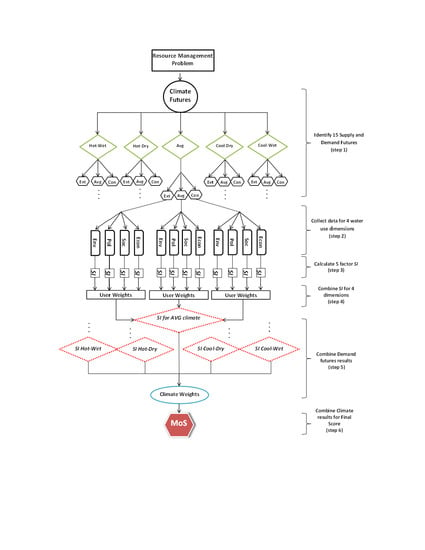
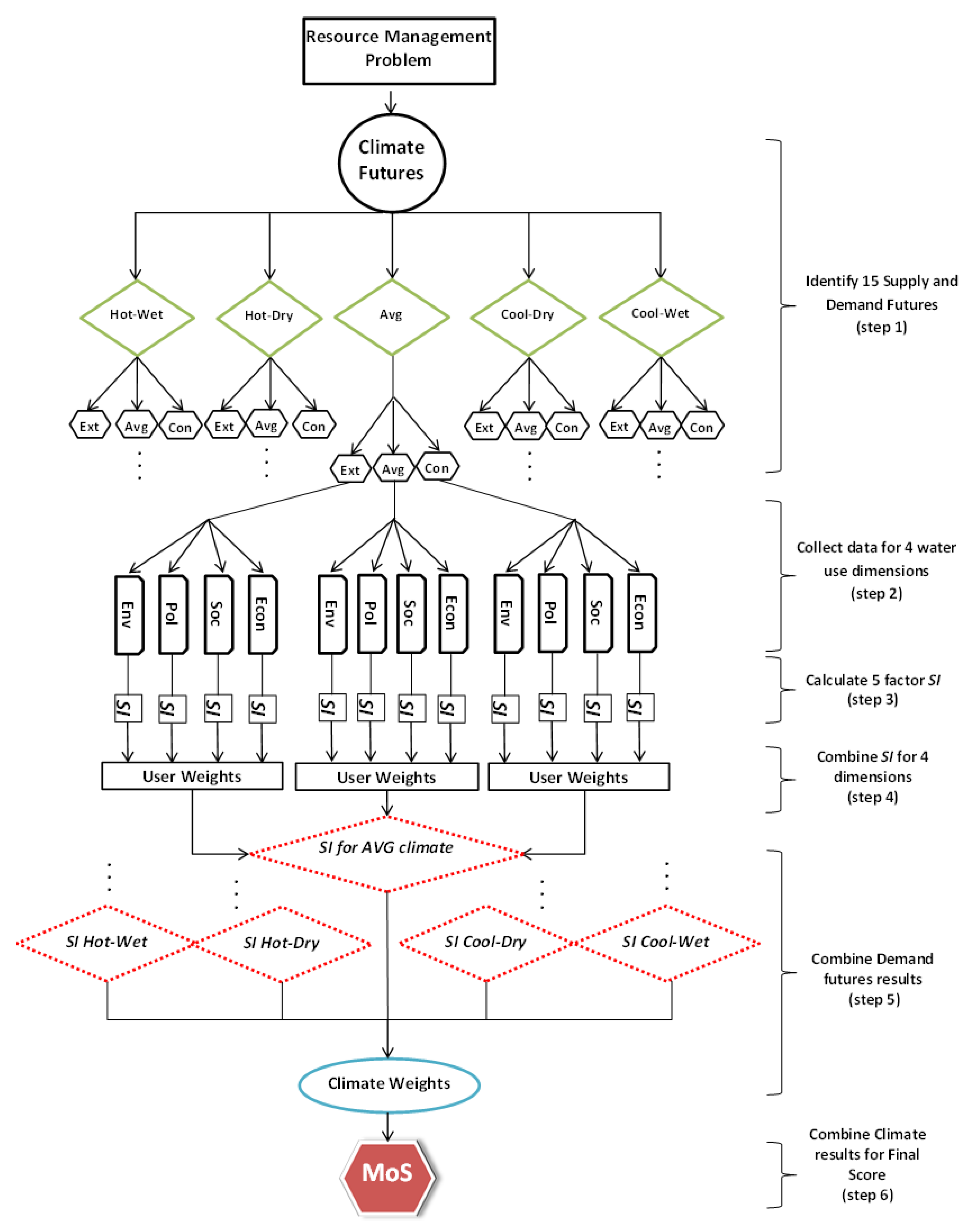
Following the MoS flow chart in Figure 3 to evaluate the functioning of the tested management plans outlined above, the constructed WEAP model was run 75 times considering three demand scenarios, five climate futures, and five management schemes. Utilizing the five-factor sustainability index outlined above (Equation (9)) to consider performance in the four different variable dimensions (environmental, economic, political, social), we obtained numerous results for each plan tested. These individual results were recorded in tables similar to that below (Table 9 shows results for water use plan 2.1). 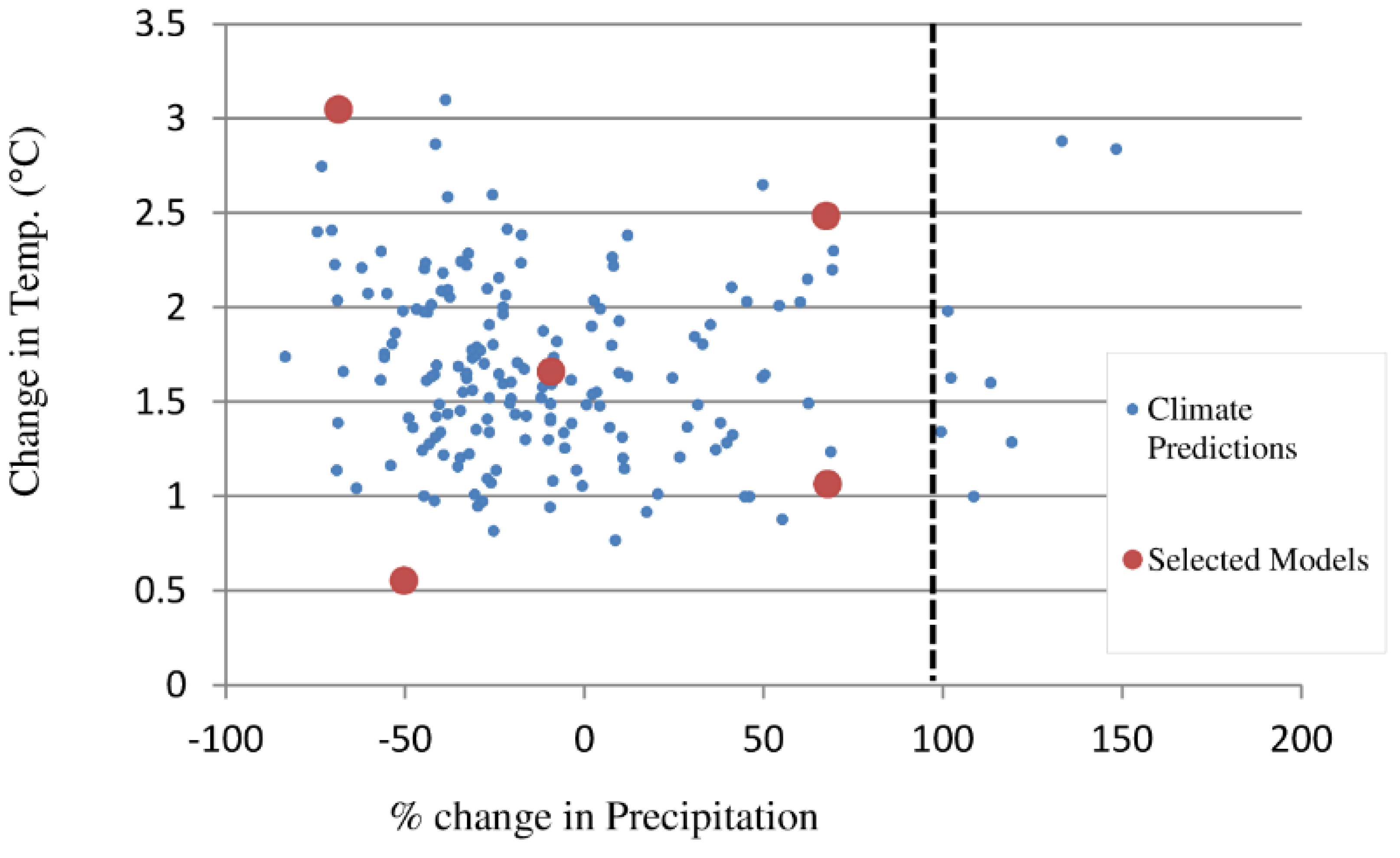To obtain a unique final value for management plan comparison and ranking, the four variable dimensions and the three demand scenarios are each given equal weight, as suggested by Loucks [31]. These weights, however, are flexible and should be adjusted according to the opinions and values of the user of the MoS algorithm. Decision-makers predicting a certain demand future over another or placing more importance in one water use sector than another might weight these as they see fit. Climate, however, should remain weighted as expressed above, as these weights are derived as a general consensus of many climate models. Considering all five-factor Sustainability Index values (Equation 9) for the 60 permutations of climate (Table 6), demand (Table 5), and dimension (Table 2), and the weightings described, the final MoS is listed in the bottom right corner of the table as a single and simple number ranging from 0 to 1 (higher values represent more desirable sustainability situations). MoS scores and relative rankings for all five management schemes are presented in Table 10.

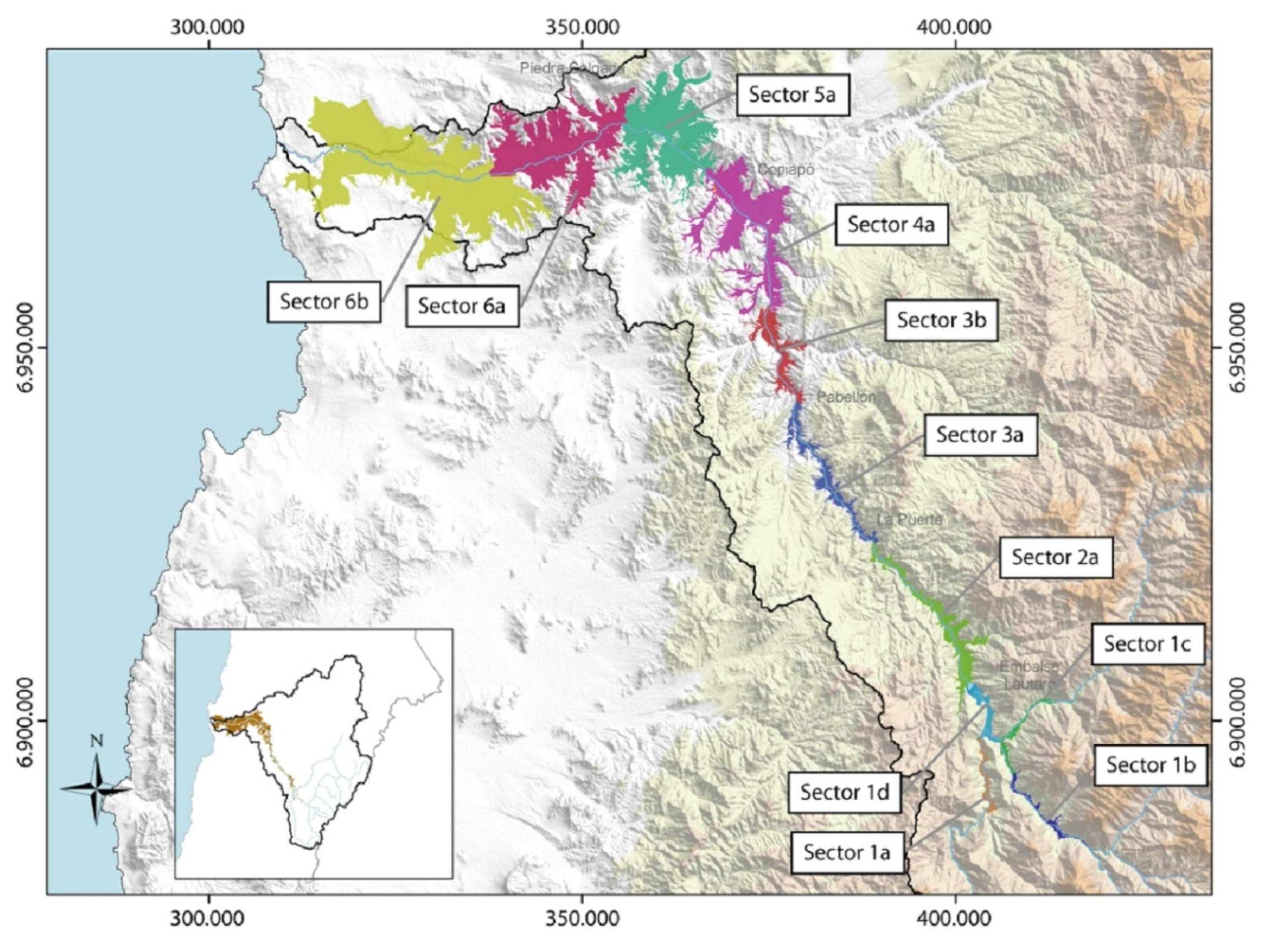
Table 8. Management schemes, original and adjusted for equal demand reduction (“sec” refers to administrative sectors, see Figure 4).

Mgmt. Plan	1.1	2.1	3.1	4.1	5.1
Old plan (Suarez et al., 2014 [40])	No reduction	All uses: 20% demand reduction	All uses: 20% demand reduction in sec 1 and 2, 35% in sec 3, 50% in sec 4	Mining/Agriculture: 30% reduction Potable: 50% demand transfer from 4a to 5a	Mining/Agriculture: 20% in sec 1 and 2, 35% in sec 3, 50% in sec 4 and 5 Potable: 50% demand transfer from 4a to 5a
Total demand Reduction	-	20%	20%	28%	27%
New Plan	No reduction	All uses: 20% demand reduction	All uses: 20% demand reduction in sec 1 and 2, 35% in sec 3, 50% in sec 4	Mining/Agriculture: 21% reduction Potable: 50% demand transfer from 4a to 5a	Mining/Agriculture: 14.4% in sec 1 and 2, 25.2% in sec 3, 36% in sec 4 and 5 Potable: 50% demand transfer from 4a to 5a
Total demand reduction	-	20%	20%	20%	20%

Table 8. Management schemes, original and adjusted for equal demand reduction (“sec” refers to administrative sectors, see Figure 4).

Mgmt. Plan	1.1	2.1	3.1	4.1	5.1
Old plan (Suarez et al., 2014 [40])	No reduction	All uses: 20% demand reduction	All uses: 20% demand reduction in sec 1 and 2, 35% in sec 3, 50% in sec 4	Mining/Agriculture: 30% reduction Potable: 50% demand transfer from 4a to 5a	Mining/Agriculture: 20% in sec 1 and 2, 35% in sec 3, 50% in sec 4 and 5 Potable: 50% demand transfer from 4a to 5a
Total demand Reduction	-	20%	20%	28%	27%
New Plan	No reduction	All uses: 20% demand reduction	All uses: 20% demand reduction in sec 1 and 2, 35% in sec 3, 50% in sec 4	Mining/Agriculture: 21% reduction Potable: 50% demand transfer from 4a to 5a	Mining/Agriculture: 14.4% in sec 1 and 2, 25.2% in sec 3, 36% in sec 4 and 5 Potable: 50% demand transfer from 4a to 5a
Total demand reduction	-	20%	20%	20%	20%

Table 9. Example table for the computation of MoS completed for each management option under Extreme (Ext), Average (Avg), and Conservative (Con) demand futures (using management scheme 2.1 as example).

Water Use (2.1)		Environmental			Economic			Political			Social
Demand Model		Ext	Avg	Con	Ext	Avg	Con	Ext	Avg	Con	Ext	Avg	Con
Climate Scenario	Dry Hot	0.198	0.218	0.226	0.077	0.344	0.449	0.207	0.492	0.732	0.638	1.000	1.000
	Dry Cool	0.213	0.231	0.239	0.080	0.346	0.455	0.209	0.506	0.900	0.630	1.000	1.000
	Wet Hot	0.204	0.224	0.231	0.078	0.345	0.450	0.199	0.493	0.772	0.615	1.000	1.000
	Wet Cool	0.198	0.230	0.238	0.077	0.345	0.453	0.207	0.518	0.839	0.630	1.000	1.000
	Average	0.208	0.227	0.234	0.079	0.345	0.452	0.202	0.498	0.780	0.630	1.000	1.000
	Weighted Total	0.207	0.228	0.235	0.079	0.345	0.453	0.205	0.502	0.819	0.629	1.000	1.000
MoS	0.475

Table 9. Example table for the computation of MoS completed for each management option under Extreme (Ext), Average (Avg), and Conservative (Con) demand futures (using management scheme 2.1 as example).

Water Use (2.1)		Environmental			Economic			Political			Social
Demand Model		Ext	Avg	Con	Ext	Avg	Con	Ext	Avg	Con	Ext	Avg	Con
Climate Scenario	Dry Hot	0.198	0.218	0.226	0.077	0.344	0.449	0.207	0.492	0.732	0.638	1.000	1.000
	Dry Cool	0.213	0.231	0.239	0.080	0.346	0.455	0.209	0.506	0.900	0.630	1.000	1.000
	Wet Hot	0.204	0.224	0.231	0.078	0.345	0.450	0.199	0.493	0.772	0.615	1.000	1.000
	Wet Cool	0.198	0.230	0.238	0.077	0.345	0.453	0.207	0.518	0.839	0.630	1.000	1.000
	Average	0.208	0.227	0.234	0.079	0.345	0.452	0.202	0.498	0.780	0.630	1.000	1.000
	Weighted Total	0.207	0.228	0.235	0.079	0.345	0.453	0.205	0.502	0.819	0.629	1.000	1.000
MoS	0.475

Table 10. MoS Scores and rankings of adjusted management plans.

New Mgmt Plan	1.1	2.1	3.1	4.1	5.1
MoS score	0.324	0.475	0.547	0.361	0.348
Ranking	5	2	1	3	4

Table 10. MoS Scores and rankings of adjusted management plans.

New Mgmt Plan	1.1	2.1	3.1	4.1	5.1
MoS score	0.324	0.475	0.547	0.361	0.348
Ranking	5	2	1	3	4

While the purpose of the MoS was to create an index able to combine the range of supply and demand futures and their impact upon numerous variables affecting different water use dimensions into a single, easily understandable number, the analysis of the individual sustainability scores such as those in Table 9 also presents results of interest. Maintaining constant one of the two variables of future scenario uncertainty (demand and climate), the variability in sustainability introduced by the other factor may be measured for each of the four water use dimensions. Comparing the change in sustainability caused by differences in demand scenario with that produced by modification of the climate future, we observe that for all four water dimensions, demand is the more influential variable (Effect on SI of demand variance/Effect of climate variance by dimension: env., 1.89; econ., 89.5; pol., 6.9; soc., 31.4; Table 11). While much attention has been placed upon the effects of climate change on water resource availability, in arid regions where water is naturally scarce, the efficient use of this resource might perhaps be a much more important determinant of future sustainability, as indicated by these numbers.

Table 11. Effect on SI caused by future variables (second variable held constant) and relative impact.

Water Use Dimension	Environmental	Economic	Political	Social
Demand	0.0272	0.3003	0.5228	0.3965
Climate	0.0144	0.0034	0.0758	0.0126
Demand/Climate	1.89	89.49	6.90	31.38

Table 11. Effect on SI caused by future variables (second variable held constant) and relative impact.

Water Use Dimension	Environmental	Economic	Political	Social
Demand	0.0272	0.3003	0.5228	0.3965
Climate	0.0144	0.0034	0.0758	0.0126
Demand/Climate	1.89	89.49	6.90	31.38

Higher-rated plans in the MoS index, however, are not necessarily the most practical solutions. Management plan implementation cost is an essential variable in decision-making and cannot be overlooked. A plan requiring 50% reduction in water demand, for example, would logically conserve more water, but without considering the costs of enacting such a measure we are unable to compare trade-offs. For the calculation of plan implementation costs, we assume that, without improvements in technological efficiency or philanthropy on the part of economic sectors, the reduction in fresh water demand must be replaced by other means. Following the suggestion of Suarez and current practices of the Candelaria Mine in Copiapó and other mines in arid Northern Chile, we propose SWRO (sea water reverse osmosis) as the source for replacement resources.

Currently, the cost of desalinating and transporting 0.5 m³/s to the Candelaria Mine, the principal mine in the river basin located at 675 m, is approximately $3 USD/m³. On the other hand, a lower cost of $1.78/m³ is estimated for production and transport of potable water to the city of Copiapó using SWRO [84]. Being that no study has yet to calculate the economic feasibility of utilizing desalinated water for agricultural purposes in Copiapó, we chose to utilize an average of the values for desalination already observed in Copiapó ($2.39/m³). While this value is approximately four times more expensive than the highly efficient Ashkalon desalination plant in Israel ($0.57/m³), it falls within international norms [85,86]. Based on projected demands for each stakeholder under the three different future demand scenarios and the associated demand reduction percentages proposed by each management plan, we calculated a first-order approximation of plan implementation costs under the above-stated desalination costs (Table 12, column 2).

Table 12. Cost and performance evaluations of new management plans. Costs are calculated using the average cost of all demand and climate scenarios.

Plan	Implementation Cost (Million $$)	Deficit Reduction Cost (Million $$)	Total Cost (Million $$)	MoS
1.1	0	15,953	15,953	0.324
2.1	6901	7718	14,619	0.475
3.1	6865	7115	13,980	0.547
4.1(new)	6671	14,935	21,606	0.361
5.1(new)	6632	7705	14,337	0.348

Table 12. Cost and performance evaluations of new management plans. Costs are calculated using the average cost of all demand and climate scenarios.

Plan	Implementation Cost (Million $$)	Deficit Reduction Cost (Million $$)	Total Cost (Million $$)	MoS
1.1	0	15,953	15,953	0.324
2.1	6901	7718	14,619	0.475
3.1	6865	7115	13,980	0.547
4.1(new)	6671	14,935	21,606	0.361
5.1(new)	6632	7705	14,337	0.348

The highest-performing management plan utilizing the traditional single-variable static approach seen in Suarez et al. (50% reduction in all demands) would also be the most expensive option to implement, costing an estimated $9.3 billion USD more than the next most expensive option [40]. Suarez et al. [40] agree upon the infeasibility of this option due to difficulty of implementation and instead propose plan 2.2 (30% reduction in all demands), which still happens to be the second most expensive option, costing an estimated $2.8 billion USD more than the next most expensive option. These additional costs over a more traditional method that employs static future demand scenarios result from the fact that even in the best case scenario, conservative demand projections are greater than current consumption.

Implementation, however, is not the only cost inherent in a management plan, but as Suarez et al. [40] correctly argue, each plan will result in a different future water deficit based upon the ability to meet demand after implementation. While Suarez’s cost calculations were a necessary first attempt to convert hydrological performance into an economic value, certain assumptions led to a large underestimation of deficit cost. The potential effects associated with assuming static futures in climate and markets have been addressed in this work, but the assumption that ex post facto deficit recovery involves the same cost as preventative resource production must also be addressed. While the nearly deterministic nature of their demands allows the mining and potable water sectors to prepare for deficits, the fact that additional water demand and deficits are calculated after the fact for agricultural purposes dependent upon stochastic rainfall limits the plausibility of desalination for deficit reduction (at the rate of $1.35–$2.01/m³ as employed by Suarez). Rather, the most likely costs to be incurred by farmers will come in the form of reduced crop yield. Taking the crop irrigation demand requirements for Copiapó [59] of 17,735 m³/ha/year, the average yield for table grape production in climatic zones similar to Copiapó [87] of 19,952 metric tons/ hectare, and the average table grape prices over the last five years for produce originating in Copiapó of $1.1/kg as reported by the Chilean Office of Agrarian Studies and Politics ODEPA [88], we find that average economic product lost by deficit is $14.85/m³. Clearly, when compared with the marginal cost of SWRO (~$2.39/m³), economic loss due to water deficit is much greater and should be avoided. Were it not possible to reutilize the desalination plants mentioned for management plan implementation, increasing their capacity so as to meet deficit needs, this new factor, combined with the dominance of deficits by the agricultural sector, would greatly raise the costs of deficit reduction and increase the importance of implementing preventative sustainability plans.

Independent of this decision to calculate crop losses or agricultural drought prevention, the accepted static futures methodology for resource analysis (e.g., [40]) underestimates deficit by a factor of more than 10 times by overlooking the projections of mainly increased demand and, to a minor extent, decreased supply. It should also be noted that although Suarez et al. [40] estimated that a 50% demand reduction would lead to aquifer recharge and thus an environmentally sustainable position, by excluding the potential effects of climate change and demand growth, they likely overstate their case. According to calculations in this study that consider these factors, even a 50% reduction in future demand, at a cost of at least $16.1 billion USD for implementation, would not be sufficient to reach absolute sustainability in Copiapó, and would still require additional expenditure for deficit reduction through SWRO. As might be seen in Table 12 below, at that cost it would be more economic to follow nearly any other management scheme, thus the consideration of future demand growth is integral to the decision-making process.

Combing the costs of implementation of the new management plans (equal percentage of demand reduction, Table 8) with the costs of deficits caused by the failure of these plans to meet demand requirements, we arrive at a first order estimation for the total cost of adopting the management plans for water resource sustainability. As might be seen in Table 12 below, plan 3.1 (previously ranked only third by Suarez et al. [40]) now not only stands as the best-performing option according to our MoS, but also is estimated to be the least expensive.

Merely by showing that results are different does not necessarily prove that the MoS methodology is any more appropriate than the traditional method which does not account for climate change, demand change, or multi-sectorial multivariable analysis. Being that these techniques are intended to aid in resource planning for uncertain futures, their sensitivity to variations in future variables is of prime concern. A more robust analysis methodology would be one that either eliminates variable uncertainty or includes the range of uncertainty into calculations. Maintaining constant the climate scenario (dry-cool, dry-hot, wet-cool, wet-hot, average), we calculate the range of total water deficit during the 30-year period over all three demand scenarios (conservative, average, extreme) (Table 13). By eliminating the effects of the climate variable, we observe that the range of uncertainty introduced by the demand variable is much greater (between 3200 and 5600 Mm³ depending on the management scheme) than the range between all management schemes using the traditional methodology (500 Mm³) observed in Suarez et al. [40]. The uncertainty caused by climate also results in a much greater range under the extreme demand scenario (1200–2000 Mm³) and also under conservative and average demand if we exclude the base scheme in which no water conservation measures are taken. In fact, by overlooking climate and demand changes altogether, the traditional method underestimates water deficits even in the best-case scenario (conservative demand and cool-wet climate future) in all but the base scenario by an average of 250%. These ranges of uncertainty introduced by variables that are overlooked by the traditional analysis technique observed in Suarez et al. [40], being greater than the range of deficit values between the potential management schemes being analyzed (experimental variable), demonstrate the need for a robust analytical methodology. Reliant upon uncontrolled stochastic variables rather than upon robust analysis makes the conclusions of the traditional method highly fragile for decision-making under an uncertain future. The MoS methodology, however, includes these uncertainties in its calculations by estimating the range of effects caused by potential futures rather than gambling on a single demand and climate scenario. Thus, the high range of potential water deficits resultant from uncertain futures, rather than introducing a conflicting variable, is incorporated into the MoS evaluation of management schemes.

Table 13. Range of deficits introduced by uncertain variables in million m³, considering either a single demand scenario over all climates or a single climate scenario over all demands. To the right are projected deficits using the traditional and MoS techniques.

Mgmt Scheme	Single Demand Scenario (All Climates Considered)			Single Climate Scenario (All Demands Considered)					All Variables Considered
	Cons.	Avg.	Ext.	Avg.	Dry-Cool	Dry-Hot	Wet-Cool	Wet-Hot	Suarez et al.	MoS
1.1	139	267	1972	5397	5275	5588	5300	5501	528	2311
2.1	52	120	1408	3982	3887	4128	3913	4052	32	1534
3.1	27	91	1364	3936	3814	4122	3841	4038	18	1438
4.1	52	789	1409	3982	3887	4122	3914	8686	54	1795
5.1	62	128	1428	3999	3925	4118	3946	4051	45	1571

Table 13. Range of deficits introduced by uncertain variables in million m³, considering either a single demand scenario over all climates or a single climate scenario over all demands. To the right are projected deficits using the traditional and MoS techniques.

Mgmt Scheme	Single Demand Scenario (All Climates Considered)			Single Climate Scenario (All Demands Considered)					All Variables Considered
	Cons.	Avg.	Ext.	Avg.	Dry-Cool	Dry-Hot	Wet-Cool	Wet-Hot	Suarez et al.	MoS
1.1	139	267	1972	5397	5275	5588	5300	5501	528	2311
2.1	52	120	1408	3982	3887	4128	3913	4052	32	1534
3.1	27	91	1364	3936	3814	4122	3841	4038	18	1438
4.1	52	789	1409	3982	3887	4122	3914	8686	54	1795
5.1	62	128	1428	3999	3925	4118	3946	4051	45	1571

While the entirety of the difference in the MoS score does not lie in a single category but rather is distributed throughout the different sustainability indicators and water use dimensions, a gain in 0.072 MoS as that observed between plans 3.1 and 2.1 is equivalent to 25.8 more months where water is provided to all water utility clients during the 30-year period, or it is equivalent to the average aquifer depth being 5.59 m closer to the surface. This 25.8-month difference in reliability multiplied by 239 clients without water on average per failure and 16.2 m³/client average monthly usage reported by Aguas Chañar, who charges approximately $1.31/m³, gives a total of $130,868 USD gained by choosing the better-performing option. The 5.59 m difference in average aquifer depth translates into a difference of $15.1 million USD extra expenditure in pumping costs during the 30-year period when choosing plan 2.1 over 3.1. According to these numbers it may be observed that the MoS does not have a strict monetary interpretation as the same reduction of 0.072 in the index score would correlate to incurred costs that vary over two orders of magnitude. This difference is to be expected, however, as potable water usage is nearly two orders of magnitude lower than total aquifer pumping. These translations of the MoS into monetary values are merely examples to aid in user understanding of the index. Nevertheless, decision-makers should be presented with both plans and costs to aid in decision-making.

5. Conclusions

Addressing issues of oversimplification of futures observed in current sustainability analysis methods, this research proposes a robust, dynamic, and multivariate approach for decision support in water resources. While the simulation of results in multiple climate and demand scenarios increases calculation cost, by evaluating the range of watershed performance in response to these uncertain parameters avoids potentially costly underestimations produced by simpler techniques. To demonstrate its application, this new methodology (the Measure of Sustainability or “MoS”) was applied to the Copiapó, Chile, watershed, an example of an arid watershed under extreme natural and anthropogenic water stress. Results of the MoS were compared to those previously calculated by a more traditional approach in which climate and water demands are considered to be stationary.

The MoS results, coupled with first order estimated costs, provide decision-makers with a simplified manner of selecting resource management possibilities whose economic feasibility might further be analyzed by financial experts. In the analysis of Copiapó we observed that the sustainability of the original plans evaluated by a more traditional approach [40] is highly dependent upon the water reduction and thus the inherent implementation cost proposed by each. Even in the best possible scenario of a conservative demand future, the traditional method of static demand underestimates the cost to implement any management scheme while overlooking the effects of climate change also misjudges the magnitude of future water deficits. Specifically in the agricultural sector, the marginal cost of crop loss due to water deficit is much greater than the marginal cost of SWRO and thus should be avoided where possible through preparation rather than remediation. This leads us to suggest further investigation into the economic feasibility of SWRO solutions for agricultural deficit mitigation.

Independently analyzing the uncertain future variables of climate and demand, we observe that the uncertainty introduced by each of these is larger than the range of the experimental variable deficit of each management scheme in the traditional methodology. In addition, we observe that in arid regions, such as Copiapó, Chile, where water resources are naturally scarce, demand variability might introduce more risk to sustainability than potential changes in climate, leading us to suggest increased efforts in hydrologic efficiency. Combining these two variables, however, to compare four management schemes with equal water reduction but different distribution structures, we were able to find that reducing all demands by a strict 20% (plan 2.1) and reducing all demands by geographic sector (plan 3.1) are the best performing management schemes, with 3.1 scoring slightly higher in the MoS index (0.072) but also costing slightly less (approximately $639 million USD). Not only for lower economic cost but also for improved performance in the Measure of Sustainability (MoS) index, we propose the adoption of plan 3.1 over Suarez et al.’s selection of 2.1 for water management in the Copiapó basin.

Mounting concerns about the impacts of human activities, potential climatic shifts, expanding populations and water demands as well as new knowledge are part of the pressing need to develop alternative management schemes in an integrated manner, particularly in environments with scarce natural resources. In this background, it is important to emphasize the transition in theory and practice from Environmental Impact Assessment to Risk Assessment, and then to Sustainability Analysis and Vulnerability Assessment. Thus, given the uncertainty of future events and the dependence upon climate and market trajectories, we reiterate that the plans selected by this methodology are not necessarily the most optimal solutions to problems in water resource sustainability. By considering the performance of each plan under the expected range of likely futures, however, the MoS methodology proposes solutions that are robust to variations in future parameter values and are thus the best management options in a stochastic natural world. While important, sustainability and cost are not the only factors that influence environmental decision-making. Social acceptance, political feasibility, and technological capabilities also influence the opinions of stakeholders and thus add a component of uncertainty in values not directly addressed by the MoS methodology. Further research in decision support should address issues of political and social will for integrated conservation measures. In particular, due to its dominance of demand, inelasticity of infrastructure, and disjointed individualist organization, the agricultural sector’s motivation to participate in water demand management should be of pressing interest for future study. As observed by considering the range of future water supply and demand trajectories, the MoS demonstrates that sustainability management is even more vital than previously thought.