
Assessing the Performance of In-Stream Restoration Projects Using Radio Frequency Identification (RFID) Transponders

Abstract
:1. Introduction
2. Methods
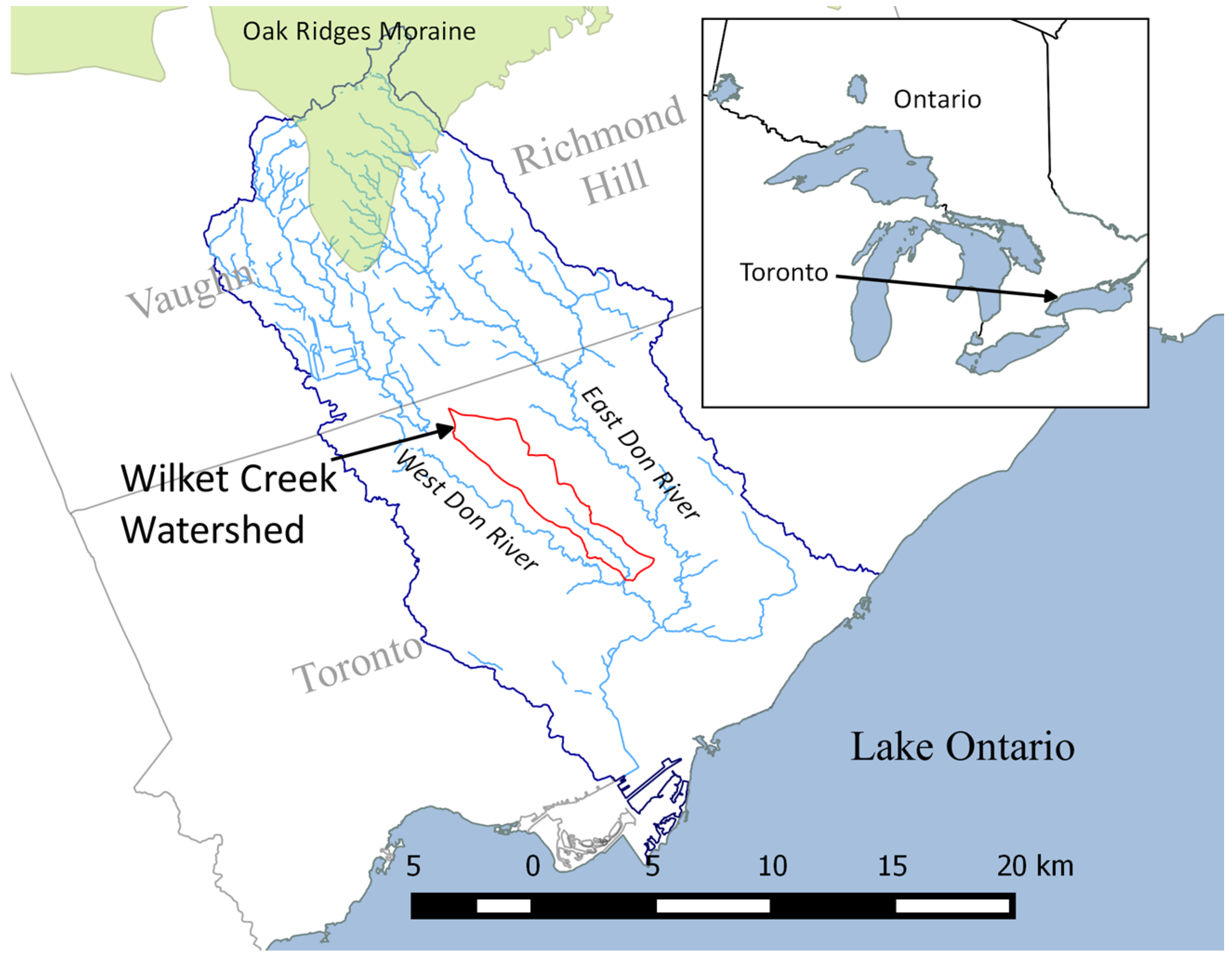
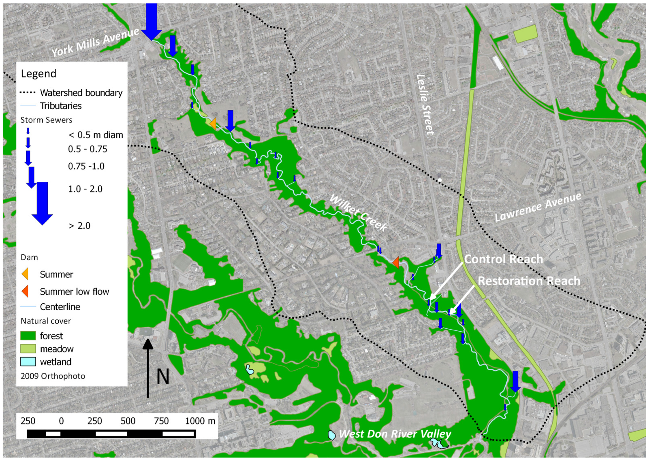
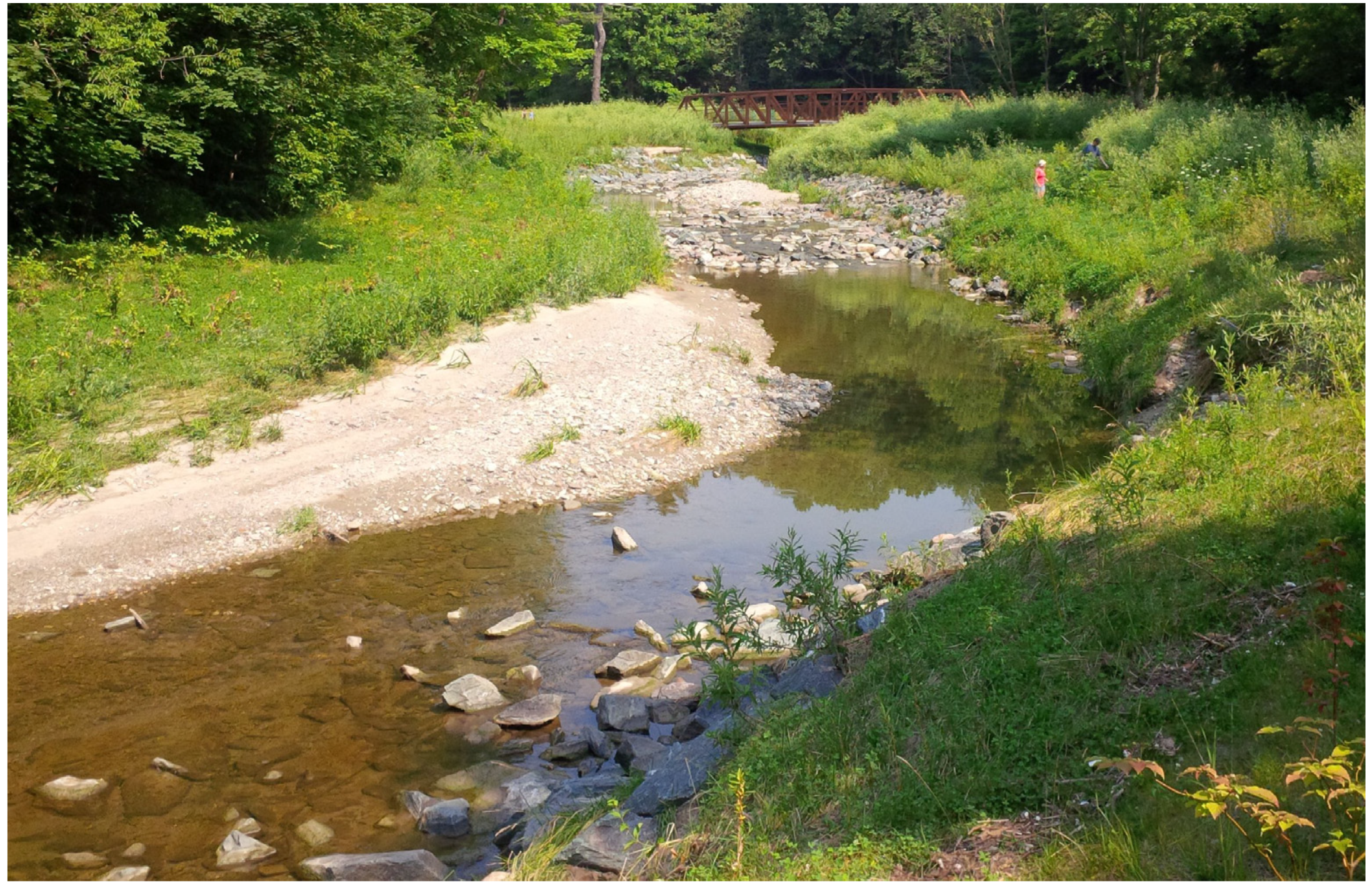
2.1. Field Site

2.2. Field Methods


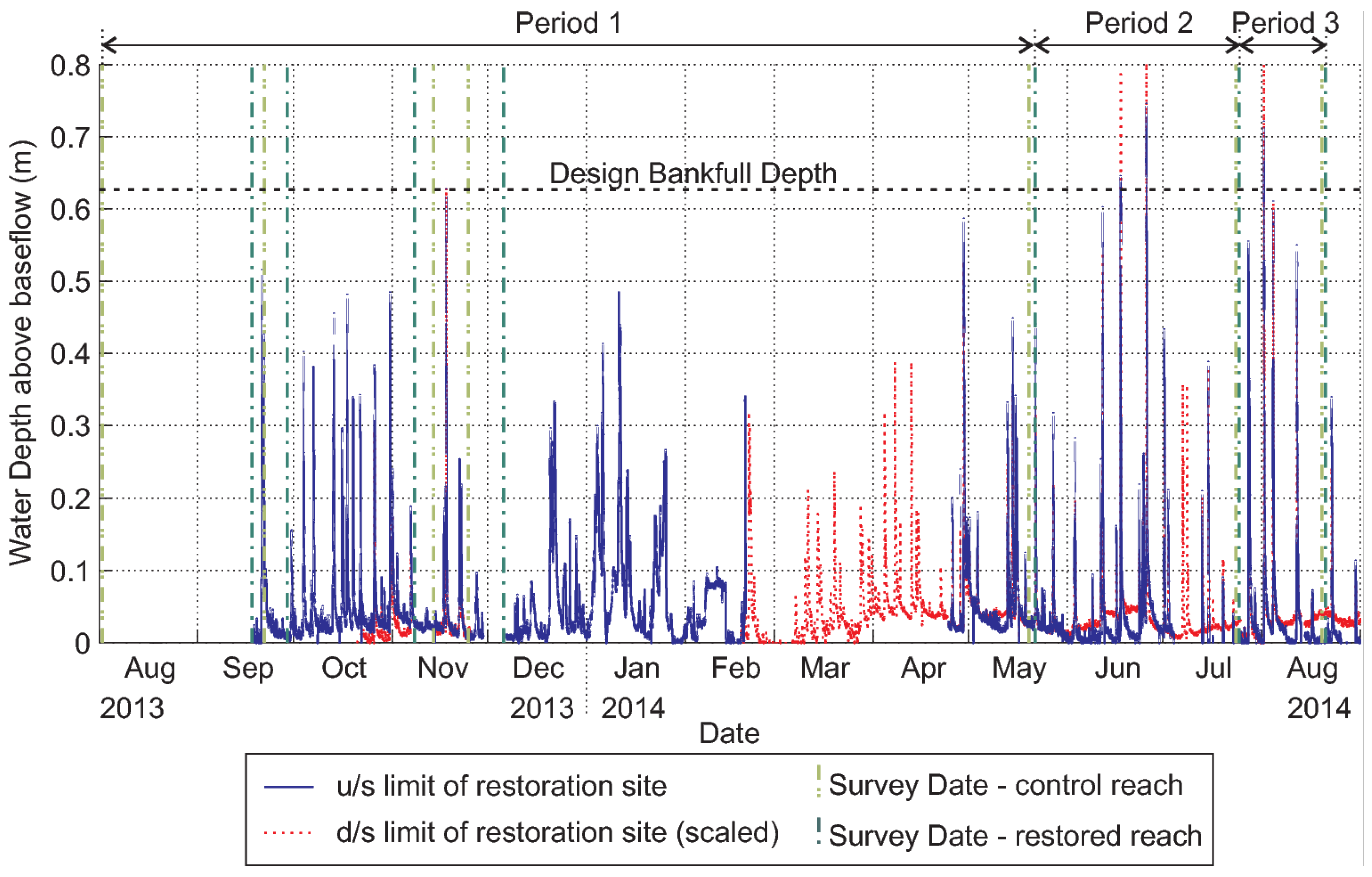
| Period | 1 | 2 | 3 |
|---|---|---|---|
| Start date | August/September 2013 | 22 May 2014 | 25 July 2014 |
| End date | 22 May 2014 | 25 July 2014 | 21 August 2014 |
| Maximum flood date | 18 November 2013 | 25 June 2014 | 1 August 2014 |
| Y (m) | 1.01 | 1.13 | 1.11 |
| τ (N/m2) | 80 | 90 | 88 |
| τ* (D50 = 58 mm) | 0.085 | 0.094 | 0.097 |
| τ* (D50 = 115 mm) | 0.043 | 0.048 | 0.047 |
2.3. Data Analysis
2.3.1. Mobility
2.3.2. Travel Distance
3. Results
3.1. Basic Particle Tracking Statistics
| Flooding Period | 1 | 2 | 3 | |||
|---|---|---|---|---|---|---|
| Reach | Control | Restoration | Control | Restoration | Control | Restoration |
| nt | 143 | 300 | 143 | 300 | 138 | 305 |
| nl | 120 | 244 | 132 | 257 | 126 | 267 |
| ninf | 7 | 16 | 0 | 7 | 0 | 0 |
| nf = nl + ninf | 127 | 260 | 132 | 264 | 126 | 267 |
| pf = nf/nt | 0.89 | 0.87 | 0.92 | 0.88 | 0.91 | 0.88 |
| nfb = nf ∪ nf (t − 1) | 127 | 260 | 122 | 242 | 122 | 253 |
| pfb = nfb/nt | 0.89 | 0.87 | 0.85 | 0.81 | 0.88 | 0.83 |
| nm | 71 | 56 | 55 | 73 | 28 | 32 |
| pm = nm/nfb | 0.56 | 0.22 | 0.45 | 0.30 | 0.23 | 0.13 |
| CIpm¯ | 0.47–0.65 | 0.17–0.27 | 0.36–0.54 | 0.24–0.36 | 0.16–0.31 | 0.09–0.17 |
| (m) | 4.2 | 3.0 | 29 | 17 | 17 | 55 |
| CID50 (m) | 1.7–11 | 1.7–5.3 | 12–70 | 5.6–52 | 10–30 | 29–100 |
| nD50 | 5 | 5 | 7 | 9 | 6 | 4 |
| nmissing | 11 | 25 | 5 | 14 | 2 | 0 |
| nlost = nt − nf − nmissing | 5 | 15 | 6 | 22 | 10 | 38 |
| nexit | 0 | 0 | 5 | 0 | 1 | 0 |
| nenter | 0 | 0 | 0 | 5 | 0 | 1 |
3.2. Spatial Results


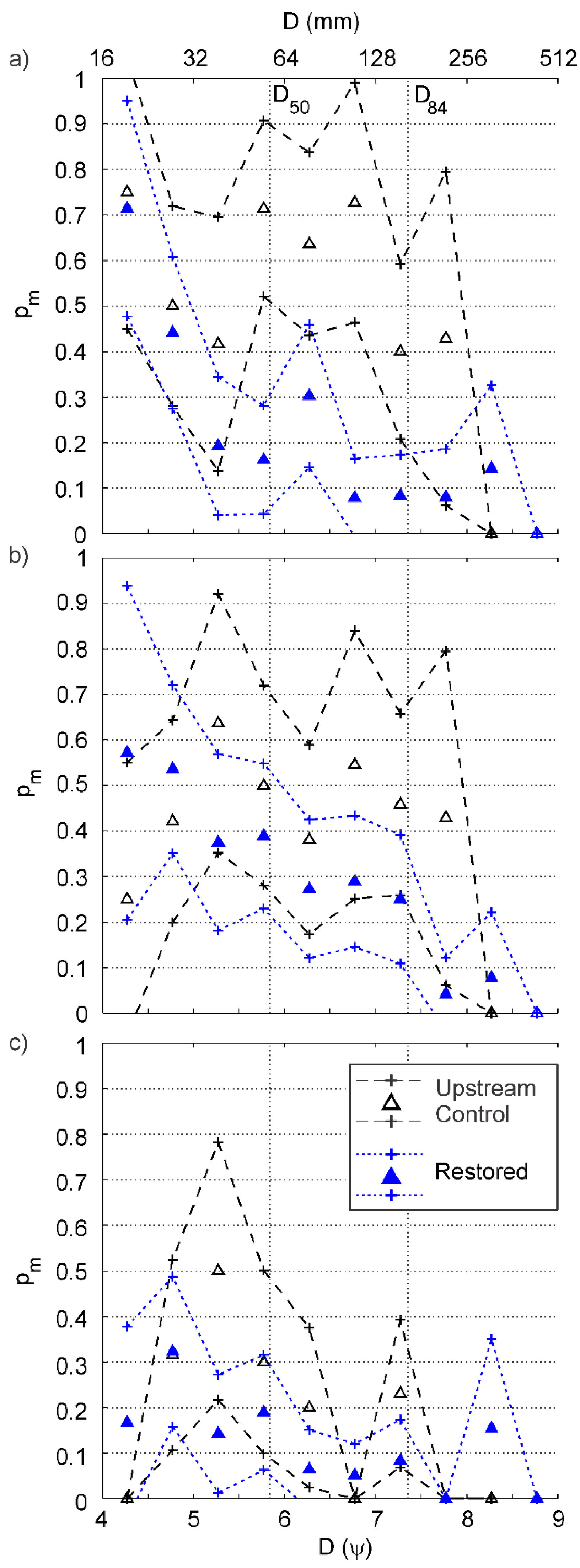
3.3. Mobility
| Period | 1 | 2 | 3 | |||
|---|---|---|---|---|---|---|
| Control | Restoration | Control | Restoration | Control | Restoration | |
| Ncategories | 8 | 9 | 8 | 9 | 8 | 9 |
| N+ | 4 | 3 | 4 | 4 | 3 | 5 |
| N− | 4 | 6 | 4 | 5 | 5 | 4 |
| Nruns | 4 | 4 | 5 | 2 | 3 | 3 |
| 5 | 5 | 5 | 5.4 | 4.8 | 5.4 | |
| 1.7 | 1.5 | 1.7 | 1.9 | 1.5 | 1.9 | |
| Hypothesis accepted? | Y | Y | Y | N | Y | Y |
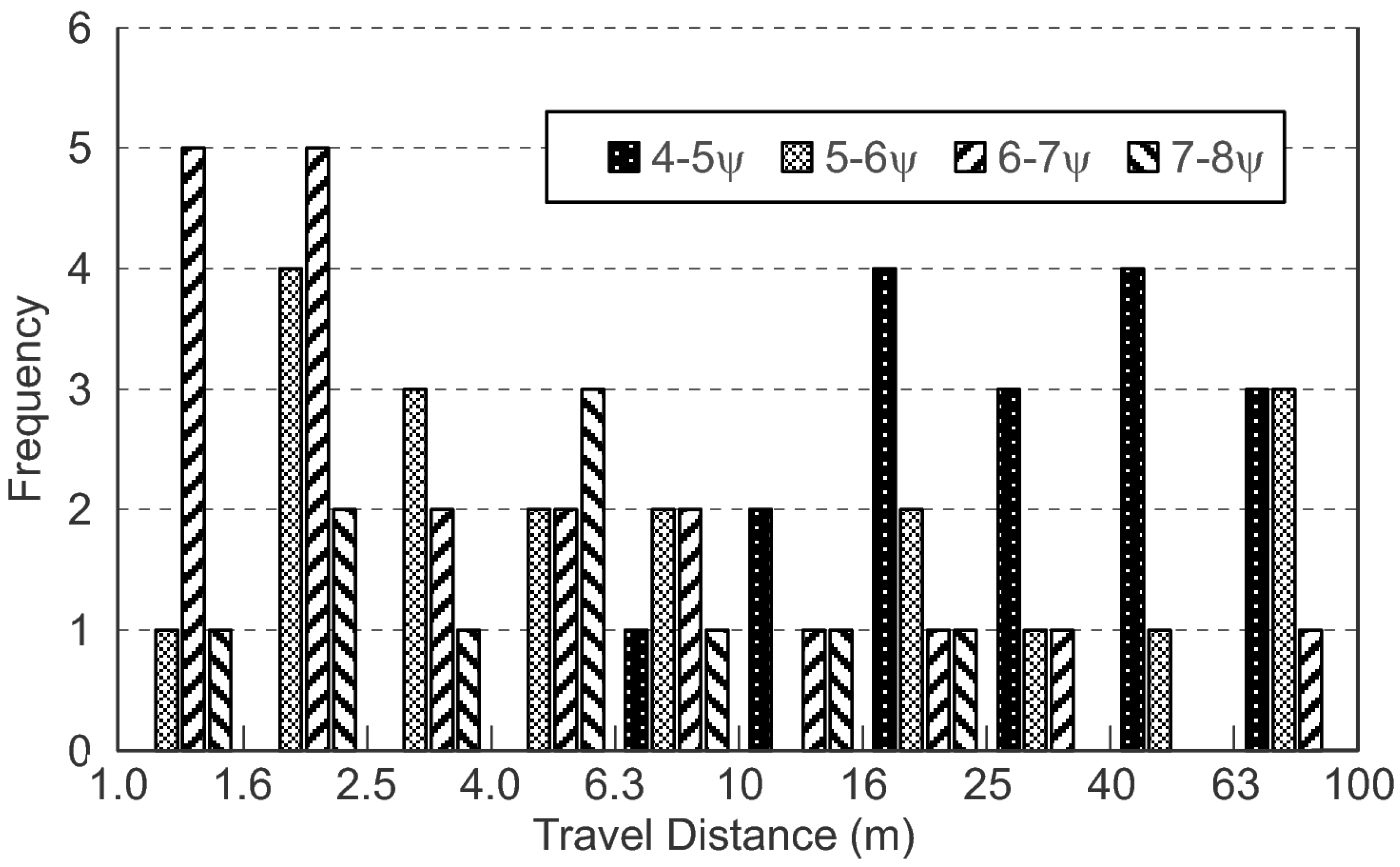
3.4. Travel Distance

4. Discussion
5. Conclusions
- Using appropriate statistical techniques, sediment tracking can be applied to compare sediment dynamics in restored and control channels as a means of assessing the effectiveness of stream restoration projects;
- The particular results of this field study demonstrate success in the sense that sediment dynamics are positively affected by the pool-riffle design. Particles in motion tend to be trapped in riffles and the mobility of larger particle sizes is reduced in comparison with a control reach even as the smaller material is scoured from the pool and transported downstream into point bars and the channel margins;
- Careful attention should be paid to sample sizes and seeding strategies in order to maximize the ability of the sediment tracking approach to distinguish differences in the sediment dynamics between reaches.
Acknowledgments
Author Contributions
Conflicts of Interest
References
- Shields, F.D.; Copeland, R.R.; Klingeman, P.C.; Doyle, M.W.; Simon, A. Design for stream restoration. J. Hydraul. Eng. 2003, 129, 575–584. [Google Scholar] [CrossRef]
- Wilcock, P.R. Stream restoration in Gravel-Bed Rivers. In Gravel-Bed Rivers VII; Church, M., Biron, P., Roy, A.G., Eds.; Wiley: Tadoussac, QC, Canada, 2012; pp. 137–146. [Google Scholar]
- Wohl, E.; Angermeier, P.L.; Bledsoe, B.; Kondolf, G.M.; MacDonnell, L.; Merritt, D.M.; Palmer, M.A.; Poff, N.L.; Tarboton, D. River restoration. Water Resour. Res. 2005, 41. [Google Scholar] [CrossRef]
- Bernhardt, E.S.; Palmer, M.A.; Allan, J.D.; Alexander, G.; Barnas, K.; Brooks, S.; Carr, J.; Clayton, S.; Dahm, C.; Follstad-Shah, J.; et al. Synthesizing US river restoration efforts. Science 2005, 308, 636–637. [Google Scholar] [CrossRef] [PubMed]
- Slate, L.O.; Shields, D.F.; Schwartz, J.S.; Carpenter, D.D.; Freeman, G.E. Engineering design standards and liability for stream channel restoration. J. Hydraul. Eng. 2007, 133, 1099–1102. [Google Scholar] [CrossRef]
- Radspinner, R.R.; Diplas, P.; Lightbody, A.F.; Sotiropoulos, F. River training and ecological enhancement potential using in-stream structures. J. Hydraul. Eng. 2010, 136, 967–980. [Google Scholar] [CrossRef]
- Downs, P.W.; Kondolf, G.M. Post-project appraisals in adaptive management of river channel restoration. Environ. Manag. 2002, 29, 477–496. [Google Scholar] [CrossRef]
- Kondolf, G.M.; Anderson, S.; Lave, R.; Pagano, L.; Merenlender, A.; Bernhardt, E.S. Two decades of river restoration in California: What can we learn? Restor. Ecol. 2007, 15, 516–523. [Google Scholar] [CrossRef]
- Bernhardt, E.S.; Sudduth, E.B.; Palmer, M.A.; Allan, J.D.; Meyer, J.L.; Alexander, G.; Follastad-Shah, J.; Hassett, B.; Jenkinson, R.; Lave, R.; et al. Restoring rivers one reach at a time: Results from a survey of U.S. river restoration practitioners. Restor. Ecol. 2007, 15, 482–493. [Google Scholar] [CrossRef]
- Miller, J.R.; Kochel, R.C. Assessment of channel dynamics, in-stream structures and post-project channel adjustments in North Carolina and its implications to effective stream restoration. Environ. Earth Sci. 2009, 59, 1681–1692. [Google Scholar] [CrossRef]
- Shields, F.D., Jr. Do we know enough about controlling sediment to mitigate damage to stream ecosystems? Ecol. Eng. 2009, 35, 1727–1733. [Google Scholar] [CrossRef]
- Morandi, B.; Piégay, H.; Lamouroux, N.; Vaudor, L. How is success or failure in river restoration projects evaluated? Feedback from french restoration projects. J. Environ. Manag. 2014, 137, 178–188. [Google Scholar] [CrossRef] [PubMed]
- Chin, A. Urban transformation of river landscapes in a global context. Geomorphology 2006, 79, 460–487. [Google Scholar] [CrossRef]
- Bernhardt, E.S.; Palmer, M.A. Restoring streams in an urbanizing world. Freshw. Biol. 2007, 52, 738–751. [Google Scholar] [CrossRef]
- Lacey, J.; Millar, R.G. Reach scale hydraulic assessment of instream salmonid habitat restoration. J. Am. Water Resour. Assoc. 2004, 40, 1631–1644. [Google Scholar] [CrossRef]
- Sear, D.A.; Newson, M.D. The hydraulic impact and performance of a lowland rehabilitation scheme based on pool-riffle installation: The River Waveney, Scole, Suffolk, UK. River Res. Appl. 2004, 20, 847–863. [Google Scholar] [CrossRef]
- Brown, R.A.; Pasternack, G.B. Comparison of methods for analysing salmon habitat rehabilitation designs for regulated rivers. River Res. Appl. 2009, 25, 745–772. [Google Scholar] [CrossRef]
- Abad, J.D.; Rhoads, B.L.; Güneralp, I.; García, M.H. Flow structure at different stages in a meander-bend with bendway weirs. J. Hydraul. Eng. 2008, 134, 1052–1063. [Google Scholar] [CrossRef]
- MacWilliams, J.M.L.; Tompkins, M.R.; Street, R.L.; Kondolf, G.M.; Kitanidis, P.K. Assessment of the effectiveness of a constructed compound channel river restoration project on an incised stream. J. Hydraul. Eng. 2010, 136, 1042–1052. [Google Scholar] [CrossRef]
- Paik, J.; Escauriaza, C.; Sotiropoulos, F. Coherent structure dynamics in turbulent flows past in-stream structures: Some insights gained via numerical simulation. J. Hydraul. Eng. 2010, 136, 981–993. [Google Scholar] [CrossRef]
- Kang, S.; Sotiropoulos, F. Large-eddy simulation of three-dimensional turbulent free surface flow past a complex stream restoration structure. J. Hydraul. Eng. 2015. [Google Scholar] [CrossRef]
- Khosronejad, A.; Hill, C.; Kang, S.; Sotiropoulos, F. Computational and experimental investigation of scour past laboratory models of stream restoration rock structures. Adv. Water Resour. 2013, 54, 191–207. [Google Scholar] [CrossRef]
- Khosronejad, A.; Kozarek, J.L.; Sotiropoulos, F. Simulation-based approach for stream restoration structure design: Model development and validation. J. Hydraul. Eng. 2014, 140. [Google Scholar] [CrossRef]
- Odgaard, A.J.; Spoljaric, A. Sediment control by submerged vanes. J. Hydraul. Eng. 1986, 112, 1164–1181. [Google Scholar] [CrossRef]
- Bhuiyan, F.; Hey, R.D.; Wormleaton, P.R. Hydraulic evaluation of W-weir for river restoration. J. Hydraul. Eng. 2007, 133, 596–609. [Google Scholar] [CrossRef]
- Bhuiyan, F.; Hey, R.D.; Wormleaton, P.R. Effects of vanes and W-weir on sediment transport in meandering channels. J. Hydraul. Eng. 2009, 135, 339–349. [Google Scholar] [CrossRef]
- Jamieson, E.C.; Rennie, C.D.; Townsend, R.D. 3D flow and sediment dynamics in a laboratory channel bend with and without stream barbs. J. Hydraul. Eng. 2013, 139, 154–166. [Google Scholar] [CrossRef]
- Kuhnle, R.A.; Alonso, C.V.; Shields, F.D. Local scour associated with angled spur dikes. J. Hydraul. Eng. 2002, 128, 1087–1093. [Google Scholar] [CrossRef]
- Thompson, D.M. Channel-bed scour with high versus low deflectors. J. Hydraul. Eng. 2002, 128, 640–643. [Google Scholar] [CrossRef]
- Bouska, K.L.; Stoebner, T.J. Characterizing geomorphic change from anthropogenic disturbances to inform restoration in the upper Cache River, Illinois. J. Am. Water Resour. Assoc. 2015, 51, 734–745. [Google Scholar] [CrossRef]
- Shields, F.D.; Cooper, C.M.; Knight, S.S. Experiment in stream restoration. J. Hydraul. Eng. 1995, 121, 494–502. [Google Scholar] [CrossRef]
- Roni, P.; Beechie, T.J.; Bilby, R.E.; Leonetti, F.E.; Pollock, M.M.; Pess, G.R. A review of stream restoration techniques and a hierarchical strategy for prioritizing restoration in Pacific Northwest watersheds. North Am. J. Fish. Manag. 2002, 22, 1–20. [Google Scholar] [CrossRef]
- Roper, B.B.; Konnoff, D.; Heller, D.; Wieman, K. Durability of Pacific Northwest instream structures following floods. N. Am. J. Fish. Manag. 1998, 18, 686–693. [Google Scholar] [CrossRef]
- Buchanan, B.P.; Nagle, G.N.; Walter, M.T. Long-term monitoring and assessment of a stream restoration project in central New York. River Res. Appl. 2014, 30, 245–258. [Google Scholar] [CrossRef]
- Poff, N.L.; Ward, J.V. Physical habitat template of lotic systems: Recovery in the context of historical pattern of spatiotemporal heterogeneity. Environ. Manag. 1990, 14, 629–645. [Google Scholar] [CrossRef]
- Thorp, J.H.; Thoms, M.C.; Delong, M.D. The riverine ecosystem synthesis: Biocomplexity in river networks across space and time. River Res. Appl. 2006, 22, 123–147. [Google Scholar] [CrossRef]
- Wilcock, P.R.; McArdell, B.W. Surface-based fractional transport rates: Mobilization thresholds and partial transport of a sand-gravel sediment. Water Resour. Res. 1993, 29, 1297–1312. [Google Scholar] [CrossRef]
- Wilcock, P.R.; McArdell, B.W. Partial transport of a sand/gravel mixture. Water Resour. Res. 1997, 33, 235–245. [Google Scholar] [CrossRef]
- Haschenburger, J.K.; Wilcock, P.R. Partial transport in a natural gravel bed channel. Water Resour. Res. 2003, 39. [Google Scholar] [CrossRef]
- Church, M.; Hassan, M.A. Mobility of bed material in Harris Creek. Water Resour. Res. 2002, 38. [Google Scholar] [CrossRef]
- Church, M.; Hassan, M.A. Size and distance of travel of unconstrained clasts on a streambed. Water Resour. Res. 1992, 28, 299–303. [Google Scholar] [CrossRef]
- Haschenburger, J.K. Tracing river gravels: Insights into dispersion from a long-term field experiment. Geomorphology 2013, 200, 121–131. [Google Scholar] [CrossRef]
- Vázquez-Tarrío, D.; Menéndez-Duarte, R. Bedload transport rates for coarse-bed streams in an Atlantic Region (Narcea River, NW Iberian Peninsula). Geomorphology 2014, 217, 1–14. [Google Scholar] [CrossRef]
- Lamarre, H.; MacVicar, B.; Roy, A.G. Using passive integrated transponder (PIT) tags to investigate sediment transport in Gravel-Bed Rivers. J. Sediment. Res. 2005, 75, 736–741. [Google Scholar] [CrossRef]
- MacVicar, B.J.; Roy, A.G. Sediment mobility in a forced riffle-pool. Geomorphology 2011, 125, 445–456. [Google Scholar] [CrossRef]
- Liébault, F.; Bellot, H.; Chapuis, M.; Klotz, S.; Deschâtres, M. Bedload tracing in a high-sediment-load mountain stream. Earth Surf. Process. Landf. 2012, 37, 385–399. [Google Scholar] [CrossRef]
- Bradley, N.D.; Tucker, G.E. Measuring gravel transport and dispersion in a mountain river using passive radio tracers. Earth Surf. Process. Landf. 2012, 37, 1034–1045. [Google Scholar] [CrossRef]
- Schneider, J.M.; Turowski, J.M.; Rickenmann, D.; Hegglin, R.; Arrigo, S.; Mao, L.; Kirchner, J.W. Scaling relationships between bed load volumes, transport distances, and stream power in steep mountain channels. J. Geophys. Res. Earth Surf. 2014, 119, 533–549. [Google Scholar] [CrossRef]
- Chapuis, M.; Dufour, S.; Provansal, M.; Couvert, B.; de Linares, M. Coupling channel evolution monitoring and RFID tracking in a large, wandering, gravel-bed river: Insights into sediment routing on geomorphic continuity through a riffle-pool sequence. Geomorphology 2015, 231, 258–269. [Google Scholar] [CrossRef]
- Houbrechts, G.; Levecq, Y.; Peeters, A.; Hallot, E.; van Campenhout, J.; Denis, A.C.; Petit, F. Evaluation of long-term bedload virtual velocity in gravel-bed rivers (Ardenne, Belgium). Geomorphology 2015. [Google Scholar] [CrossRef]
- Arnaud, F.; Piégay, H.; Vaudor, L.; Bultingaire, L.; Fantino, G. Technical specifications of low-frequency radio identification bedload tracking from field experiments: Differences in antennas, tags and operators. Geomorphology 2015, 238, 37–46. [Google Scholar] [CrossRef]
- Biron, P.M.; Carver, R.B.; Carré, D.M. Sediment transport and flow dynamics around a restored pool in a fish habitat rehabilitation project: Field and 3D numerical modelling experiments. River Res. Appl. 2011, 28, 926–939. [Google Scholar] [CrossRef]
- Krapesch, G.; Tritthart, M.; Habersack, H. A model-based analysis of meander restoration. River Res. Appl. 2009, 25, 593–606. [Google Scholar] [CrossRef]
- Habersack, H.; Jäger, E.; Hauer, C. The status of the Danube River sediment regime and morphology as a basis for future basin management. Int. J. River Basin Manag. 2013, 11, 153–166. [Google Scholar] [CrossRef]
- Chapuis, M.; Bright, C.J.; Hufnagel, J.; Macvicar, B. Detection ranges and uncertainty of passive radio frequency identification (RFID) transponders for sediment tracking in gravel rivers and coastal environments. Earth Surf. Process. Landf. 2014, 39, 2109–2120. [Google Scholar] [CrossRef]
- Parish Geomorphic. TRCA Wilket Creek Emergency Works (Sites 6&7)—Technical Design Brief. Available online: http://trca.on.ca/the-living-city/green-infrastructure-projects/environmental-assessment-projects/wilket-creek-rehabilitation-project.dot. (accessed on 14 October 2015).
- Bevan, V. The Effect of Urbanisation on Sediment Supply and Transport: A Field Study of Wilket Creek in Toronto. Master’s Thesis, University of Waterloo, Waterloo, ON, Canada, 28 August 2014; p. 157. [Google Scholar]
- Heritage, G.L.; Milan, D.J.; Large, A.R.G.; Fuller, I.C. Influence of survey strategy and interpolation model on DEM quality. Geomorphology 2009, 112, 334–344. [Google Scholar] [CrossRef]
- Parker, G. Transport of gravel and sediment mixtures. In Sedimentation Engineering: Processes, Management, Modeling, and Practice; Garcia, M.H., Ed.; ASCE: Reston, VA, USA, 2008; pp. 165–252. [Google Scholar]
- Buffington, J.M.; Montgomery, D.R. A systematic analysis of eight decades of incipient motion studies with special reference to gravel-bedded rivers. Water Resour. Res. 1997, 33, 1993–2029. [Google Scholar] [CrossRef]
- Collett, D. Modelling Binary Data, 2nd ed.; Chapman and Hall/CRC: Boca Raton, FL, USA, 2002; p. 387. [Google Scholar]
- Wald, A.; Wolfowitz, J. On a test whether two samples are from the same population. Ann. Math. Stat. 1940, 11, 147–162. [Google Scholar] [CrossRef]
- Goddard, S.D.; Genton, M.G.; Hering, A.S.; Sain, S.R. Evaluating the impacts of climate change on diurnal wind power cycles using multiple regional climate models. Environmetrics 2015, 26, 192–201. [Google Scholar] [CrossRef]
- Fonseca, M.S.; Kenworth, W.J.; Griffith, E.; Hall, M.O.; Finkbeiner, M.; Bell, S.S. Factors influencing landscape pattern of the seagrass halophila decipiens in an oceanic setting. Estuar. Coast. Shelf Sci. 2008, 76, 163–174. [Google Scholar] [CrossRef]
- Wilcock, P.R. Entrainment, displacement and transport of tracer gravels. Earth Surf. Process. Landf. 1997, 22, 1125–1138. [Google Scholar] [CrossRef]
- Ferguson, R.I.; Bloomer, D.J.; Hoey, T.B.; Werritty, A. Mobility of river tracer pebbles over different timescales. Water Resour. Res. 2002, 38. [Google Scholar] [CrossRef]
- Parker, G.; Klingeman, P.C.; MacLean, D.G. Bedload and size distribution in paved gravel-bed streams. J. Hydraul. Div. 1982, 108, 544–571. [Google Scholar]
- Sear, D.A. Sediment transport processes in pool-riffle sequences. Earth Surf. Process. Landf. 1996, 21, 241–262. [Google Scholar] [CrossRef]
- MacWilliams, M.L.J.; Wheaton, J.M.; Pasternack, G.B.; Street, R.L.; Kitanidis, P.K. Flow convergence routing hypothesis for pool-riffle maintenance in alluvial rivers. Water Resour. Res. 2006, 42. [Google Scholar] [CrossRef] [Green Version]
- Milan, D.J. Sediment routing hypothesis for pool-riffle maintenance. Earth Surf. Process. Landf. 2013, 38, 1623–1641. [Google Scholar] [CrossRef]
- Thompson, D.M.; Wohl, E.E. The linkage between velocity patterns and sediment entrainment in a forced-pool and riffle unit. Earth Surf. Process. Landf. 2009, 34, 177–192. [Google Scholar] [CrossRef]
- Bridge, J.S.; Jarvis, J. The dynamics of a river bend: A study in flow and sedimentary processes. Sedimentology 1982, 29, 499–541. [Google Scholar] [CrossRef]
- Jackson, W.L.; Beschta, R.L. A model of two-phase bedload transport in an Oregon coast range stream. Earth Surf. Process. Landf. 1982, 7, 517–527. [Google Scholar] [CrossRef]
© 2015 by the authors; licensee MDPI, Basel, Switzerland. This article is an open access article distributed under the terms and conditions of the Creative Commons Attribution license (http://creativecommons.org/licenses/by/4.0/).
Share and Cite
MacVicar, B.; Chapuis, M.; Buckrell, E.; Roy, A. Assessing the Performance of In-Stream Restoration Projects Using Radio Frequency Identification (RFID) Transponders. Water 2015, 7, 5566-5591. https://doi.org/10.3390/w7105566
MacVicar B, Chapuis M, Buckrell E, Roy A. Assessing the Performance of In-Stream Restoration Projects Using Radio Frequency Identification (RFID) Transponders. Water. 2015; 7(10):5566-5591. https://doi.org/10.3390/w7105566
Chicago/Turabian StyleMacVicar, Bruce, Margot Chapuis, Emma Buckrell, and André Roy. 2015. "Assessing the Performance of In-Stream Restoration Projects Using Radio Frequency Identification (RFID) Transponders" Water 7, no. 10: 5566-5591. https://doi.org/10.3390/w7105566