Catchment-Scale Modeling of Nitrogen Dynamics in a Temperate Forested Watershed, Oregon. An Interdisciplinary Communication Strategy

Abstract

We present a systems modeling approach to the development of a place-based ecohydrological model. The conceptual model is calibrated to a variety of existing observations, taken in watershed 10 (WS10) at the HJ Andrews Experimental Forest (HJA) in Oregon, USA, a long term ecological research (LTER) site with a long history of catchment-scale data collection. The modeling framework was designed to help document and evaluate an evolving understanding of catchment processing of water, nitrogen, and carbon that has developed over the many years of on-going research at the site. We use the dynamic model to capture the temporal variation in the N and C budgets and to evaluate how different components of the complex system may control the retention and release of N in this pristine forested landscape. Results indicate that the relative roles of multiple competing controls on N change seasonally, between periods of wet/dry and growth/senescence. The model represents a communication strategy to facilitate dialog between disciplinary experimentalists and modelers, to produce a more complete picture of nitrogen cycling in the region. We view this explicit development of complete, yet conceptually simplified models as a useful and important way to evaluate complex environmental dynamics.

1. Introduction

Human-induced changes to global biogeochemical cycles are large, having for example effectively doubled the global rate of annual N fixation [1] yet the ultimate response of ecosystems to these changes remains unclear. This lack of clarity is due in part to the inter-dependencies and feedbacks between system components as well as to an incomplete understanding of the complex processes governing biogeochemical cycles. These relationships result in the inherent complexity and non-linearity of environmental systems. Components comprising environmental systems include functionally discreet entities like the atmosphere, vegetation, and soils; spatial assemblages of these entities, including hillslopes, riparian transitions, and instream environments; and also the different elements that cycle through them, including nitrogen, carbon, water, and a host of others. The detailed study of each of these individual units tends to be well-covered by traditional disciplines, such as hillslope hydrology, aquatic ecology, soil biogeochemistry, forest ecology, etc., but with less attention given to the relationships between components. That these dependencies, in some sense by definition, fall at interfaces between traditional disciplinary boundaries is an ongoing challenge for ecosystem science, though the emergence of cross-cutting disciplines, such as ecohydrology and hydrobiogeochemistry, is an indication that this challenge is being addressed. The use of numerical models, which are designed to capture relationships between system components, represents one method that can be used to contribute to our understanding of how ecosystems function, and how they may respond to future change in both climate and landcover.

The retention and release of N from temperate forested ecosystems provides a clear example of this need for understanding, at an integrated catchment scale. Its relevance is, of course, well established, with tremendous progress having been made throughout the last three decades [2,3,4]. Much of this progress has been driven by the need to better understand the response of forested catchments, which are commonly limited by N, to environmental changes, including climate change, disturbance, and increased N deposition [5]. Increasing N deposition provides a useful example, where the potential effects have been succinctly synthesized as the “nitrogen saturation” hypothesis [5,6]. Under this hypothesis, the chronically increased rates of N deposition invoke a variety of ecosystem responses, culminating in increased nitrate mobility in soils, nutrient imbalances in vegetation, forest decline, the acidification of soils, as well as increased surface water N loading leading to the potential for both acidification and eutrophication [5]. Numerous catchment scale experiments have been developed to test the saturation hypothesis [7,8], and along with them, models have been developed to predict the response of catchments to different deposition patterns [9]. Because nitrate in solution is the dominant form of N lost from these systems, the models that have been developed tend to emphasize inorganic N (e.g., [10]).

Despite the strides made in understanding catchment nitrogen cycling under the saturation hypothesis, in many temperate forested catchments, notably those on the Western side of both North and South America, current N deposition rates remain similar to those found historically [11]. In these areas that lie outside of urban or other point sources of atmospheric nitrogen, N continues to be a major limiting nutrient, losses of plant-available N remain very low, and nitrogen saturation is not currently part of the developmental trajectory [12]. The models that have been developed in regions of excess N deposition are not necessarily applicable in these places, a fact that underscores the suitability of low deposition regions as a useful counterpoint in the evaluation of ecosystem N cycling.

The HJ Andrews Experimental forest (HJA) in the Pacific Northwest of the USA is one such region. A variety of studies, based in small watersheds at HJA, and focused on different components of the nitrogen cycle have been developed since its inception in the 1960s. The synthesis of these various disciplinary studies is an ongoing effort. The application and development of a conceptual numerical model, which attempts to incorporate key components of the evolving understanding of N dynamics, provides an opportunity to inject some temporal dynamism into the ecosystem budget approach, and in this sense, contribute to the overall direction of field-based research and interpretation.

The overall objective of this paper is to outline a model formulated to describe the processes controlling N cycling in low deposition, small and primarily coniferous forest watersheds at HJA. The basis for this objective is twofold. First, some potential factors associated with the low deposition nature of the region are not explicitly captured by the current suite of standard ecosystem models. These include the relative importance of losses of organic nitrogen, as well as the potential importance of instream processing of nitrogen, and epiphytic and asymbiotic nitrogen fixation. Second, a range of disciplinary experimentalists, ranging from forest ecologists to soil biogeochemists to hillslope hydrologists and aquatic biologists collect data and develop expertise at the site. Much of this expertise has a direct bearing on nitrogen cycling, yet because it emerges from different disciplines it has been difficult to integrate it and develop a more complete understanding of the ecosystem as a whole. The model has been developed to explicitly capture a temporally dynamic N budget, by directly capturing observed rates and states that operate at HJA and forests like it (Figure 1).

The model represents a communication strategy to facilitate dialog between disciplinary experimentalists, to produce a more complete picture of nitrogen cycling in the region. This kind of modeling has seen recent growth in the environmental sciences [13,14] and we view this explicit development of complete, yet conceptually simplified models as a mechanism to more fully evaluate complex environmental dynamics. In particular, our work contributes to the idea that conceptual systems modeling can contribute to interdisciplinary science as a means of providing the capacity for individual researchers to contribute to evolving models of complex systems [13]. The models that result from such a process are not necessarily designed as predictive tools, but instead as a means to document key system details and how components may interact. Such a model may provide a useful point to begin the development of predictive modeling tools, either through detailed sensitivity and uncertainty analysis, or through the development of process-based algorithms. Nonetheless, roughly calibrated conceptual models, like we present here, present a useful framework for discussion.

Figure 1. A flow chart outlining key model stocks and fluxes. Some minor flux terms have been left out of the figure to improve clarity. Note also that the litter input into aquatic biomass is derived directly from the stocks of foliage and branches/coarse wood.

Figure 1. A flow chart outlining key model stocks and fluxes. Some minor flux terms have been left out of the figure to improve clarity. Note also that the litter input into aquatic biomass is derived directly from the stocks of foliage and branches/coarse wood.

2. Materials and Methods

2.1. Ecosystem Modeling

A wide variety of models have been developed to evaluate questions related to nitrogen dynamics, with the variation primarily manifested as different levels of complexity, different scales of application, and different questions of interest. These range from 3-dimensional physically-based research models, which are applicable across a broad range of environments and time scales (ecosys; [14]) to lumped data-based techniques (UNERF; [15]), which are reliant upon long term input output measurements, and maintain no physical basis. In this paper we are primarily interested in forested watershed nitrogen dynamics, which represents only a small subset of this broad range of models. For these ecosystems, modeling strategies generally incorporate associated carbon and water cycling, and while there is considerable overlap, the models tend to focus on one of three basic lines of inquiry. The first of these relates to forest productivity and succession. Productivity models are developed primarily to predict the successional evolution of above ground biomass (e.g., 3PG [16]) or focus on carbon dynamics and primary productivity (e.g., the PnET models [17]). Models in this group tend to include a more robust depiction of primary production, canopy processes, and carbon allocation, with somewhat less detail in terms of soil organic matter processing. The second general class of ecosystem models focuses more heavily on soil nutrient cycling and soil organic matter (SOM) dynamics. This group includes many of agricultural models, some of which have been adapted to represent forested landscapes (CENTURY [18]). A third approach focuses not on vegetation or SOM properties, but rather on hydrology and nitrogen export in an effort to provide a predictive tool to quantify nitrogen leaching potential (MERLIN [10]).

Regional to global scale biogeochemical models, a somewhat different class of simulation tools make use of many of the concepts outlined in the models above, coupling water, carbon, and nitrogen cycles to represent complete regional scale ecosystems. These models display less disciplinary focus, and are used primarily to evaluate the function of whole ecosystems under changing climate or deposition patterns. Representative models in this group include GEM [19] and BIOM-BGC [20] and INCA [21].

Most of these ecosystem scale models maintain a spatially lumped approach, though a number of spatially distributed simulation tools—those that include lateral interaction terms—have been developed (e.g., RHYSSYS [22]). With the exception of MEL [23] none of these models treat the production or mobility of dissolved organic nitrogen, an oversight representing a potentially significant structural error in terms of potential maximum amounts of sequestered carbon [23]. Additionally, while a variety of aquatic simulation models have been developed [2], these concepts have not been explicitly included in any of the ecosystem models.

The modeling we developed here relies fundamentally upon a variety of ideas and algorithms proposed within the range of existing ecosystem models. Our intention isn’t to replace any of these models, but rather to select elements from them, and to put those elements together to represent a particular location with a particular set of processes.

2.2. Study Site

The HJ Andrews Experimental Forest (HJA) Watershed 10 (WS10) is located in the western Cascades of Oregon. Soils are predominantly composed of weakly developed Inceptisols with local areas of Alfisols and Spodsols made up of thick organic horizons over weathered parent materials [24]. The geology of WS10 is characterized by Miocene volcanics, primarily breccia and massive tuff, predominate [25]. Glacial, alluvial, and mass movement processes have resulted in a deeply dissected, locally steep drainage with highly variable regolith depths [25]. Vegetation is primarily comprised by Douglas-fir (Pseudotsuga menziesii), western hemlock (Tsuga heterophylla), and western red cedar (Thuja plicata). Average annual precipitation ranges from 2300 mm at lower elevations to over 3550 mm at the highest elevations and the climate is Mediterranean, with wet mild winters characterized by long duration low to moderate intensity frontal storms. WS10 is rather unique in that a significant debris flow in 1996 effectively removed the entire riparian area and most of the stream channel currently flows on bedrock. We limit our model explorations in WS10 to the pre-1996 period, when the riparian area was intact. A more complete description of WS10 and other small watersheds at HJA is provided in [26].

Over the 55 years of small watershed studies HJA, researchers have investigated recurring themes including material and elemental budgets, forest hillslope-stream interactions, biogeochemical and hydrologic responses to disturbances, and forest ecology. Framing this long-term research is a unique long term dataset documenting the seasonal input/output response, including organic and inorganic nitrogen and water, of six small catchments for over 30 years [27]. In this paper, we focus on one of the small catchments, WS10, where terrestrial [28,29] and aquatic [30] elemental budgets have previously been developed. These studies provide a key set of measurements which we revisit in this paper as calibration and evaluation terms for the numerical model.

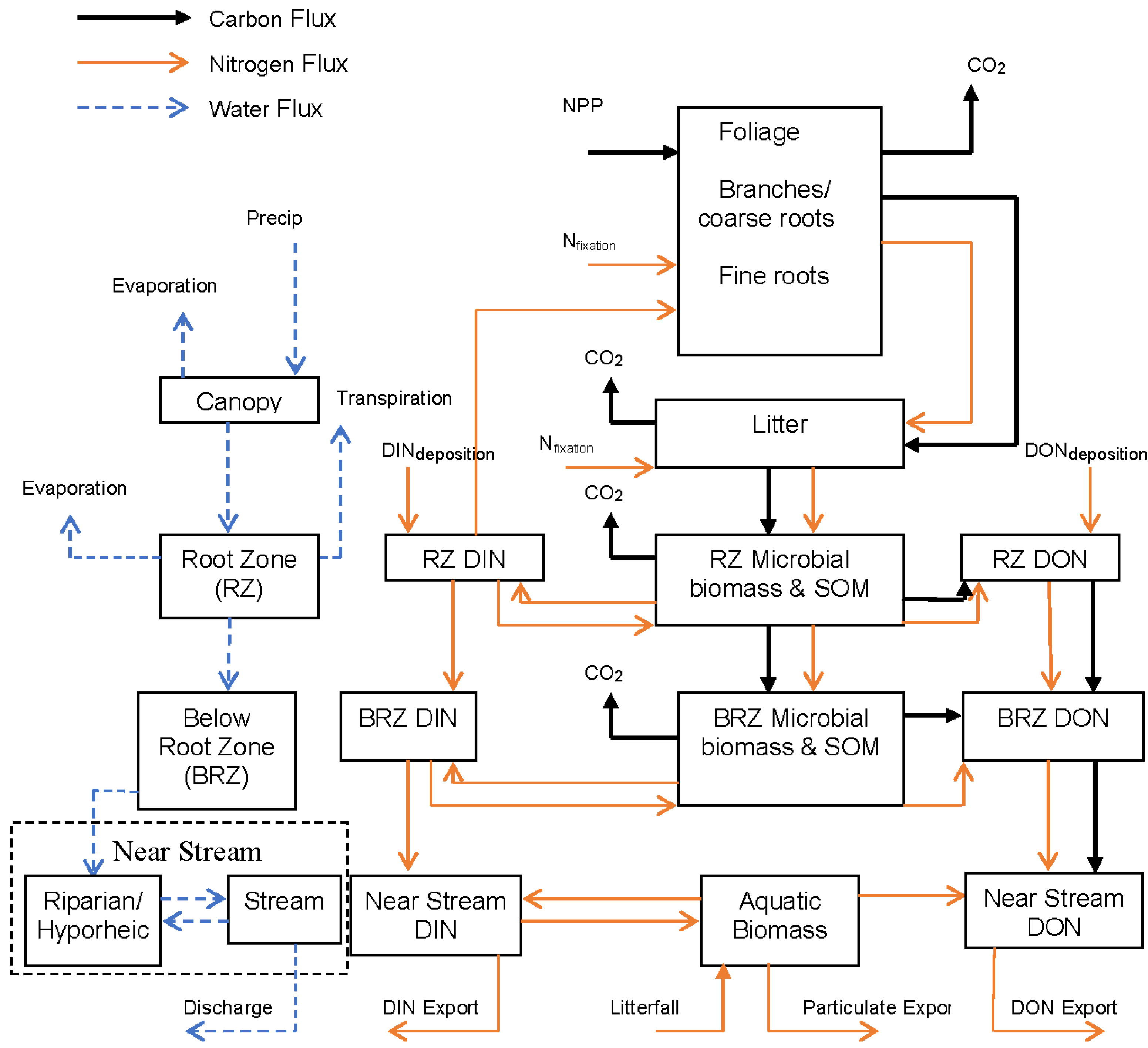
2.3. The HJA-N Model

The HJA-N model is cast as a set of mass balance equations, and uses various strategies to represent rate terms. The formulation is designed to explicitly track fluxes and masses that pass through a set of roughly defined environmental storages, differentiated in both vertical and lateral terms. It is a dynamic model that incorporates transient input data at monthly time steps, and as such is useful for evaluating potential effects of seasonality on N cycling and long term trends in N cycling in response to environmental disturbances including climate change, increasing CO₂ concentration, and large scale vegetation manipulation. It is, however, not currently designed for the short time scales necessary to consider the time scale of storm events. Table 1 outlines the naming convention used in tables outlining the model. The full list of mass balance equations is included in Table 2, with the rate terms outlined in Table 3, Table 4, Table 5 and Table 6. Model parameters are listed in Table 7 and Table 8. The model was implemented using the Stella^© systems modeling framework [31] to more fully communicate the developing model structure with the disciplinary experts providing the perceptual model of catchment process.

Table 1. Definition of naming convention used in the mathematical description of the model. Terms used in rate equations follow the form: Component_{Mass,Location}.

System Component		Mass		Additional Information
Name	Short Name	Name	Short Name	Short Name	Name
Biomass	B	Carbon	C	Root Zone	R
Detritus	D	Particulate Nitrogen	N	Below Root Zone	B
Soil Organic Matter (SOM)	S	Available Nitrogen (DIN)	Na	Hyporheic Zone	HY
		Unavailable Nitrogen (DON)	Nu	In stream/aquatic	IS
Aquatic Biomass	A	Water	Wa	Canopy	C
				Wood	w
				Fine root	r
				Foliage	f

Table 1. Definition of naming convention used in the mathematical description of the model. Terms used in rate equations follow the form: Component_{Mass,Location}.

System Component		Mass		Additional Information
Name	Short Name	Name	Short Name	Short Name	Name
Biomass	B	Carbon	C	Root Zone	R
Detritus	D	Particulate Nitrogen	N	Below Root Zone	B
Soil Organic Matter (SOM)	S	Available Nitrogen (DIN)	Na	Hyporheic Zone	HY
		Unavailable Nitrogen (DON)	Nu	In stream/aquatic	IS
Aquatic Biomass	A	Water	Wa	Canopy	C
				Wood	w
				Fine root	r
				Foliage	f

Table 2. The mass balance equations (differential equations) used to define the HJA-N model.

Equation	Defines
$\frac{d{B}_{Ci}}{dt}=P_{Ci}-T_{Ci}\to wherei=foliage,wood,fine\cdot roots$	Carbon in biomass
$\frac{d{B}_{Ni}}{dt}=U_{if}+F{S}_{Ni}-T_{Ni}\to wherei=foliage,wood,fine\cdot roots$	Nitrogen in biomass
$\frac{d{D}_{Ci}}{dt}=T_{Ci}-D_{Ci}-R_{Ci,D}\to wherei=foliage,wood,fine\cdot roots$	Carbon in detritus
$\frac{d{D}_{if}}{dt}=F{A}_{Ni}+T_{Ni}-D_{Ni}\to wherei=foliage,wood,fine\cdot roots$	Nitrogen in detritus
$\frac{d{S}_{C,R}}{dt}=D_{Cr}+D_{Cw}+D_{Cf}-R_{C,R}-T_C$	Carbon in the root zone SOM
$\frac{d{S}_{N,R}}{dt}=D_{Nr}+D_{Nw}+D_{Nf}-M_{Nu,R}-M_{Na,R}-T_N+I_{Na,R}$	Nitrogen in the root zone SOM
$\frac{d{S}_{C,B}}{dt}=T_C-R_{C,B}$	Carbon below the root zone SOM
$\frac{d{S}_{N,B}}{dt}=T_N-M_{Na,B}-M_{Nu,B}+I_{Na,B}$	Nitrogen below the root zone SOM
$\frac{d{W}_{Na,R}}{dt}=D{P}_{Na}+D_{Nu,R}+M_{Na,R}-U_{Na}-D{N}_{Na,R}-I_{Na,R}-Q_{Na,R}$	Dissolved available nitrogen in the root zone
$\frac{d{W}_{Nu,R}}{dt}=D{P}_{Nu}+M_{Nu,R}-D_{Nu,R}-Q_{Nu,R}$	Dissolved unavailable nitrogen in the root zone
$\frac{d{W}_{Na,B}}{dt}=Q_{Na,R}+D_{Nu,B}+M_{Na,B}-Q_{Na,B}-D{N}_{Na,B}-I_{Na,B}$	Dissolved available nitrogen below the root zone
$\frac{d{W}_{Nu,B}}{dt}=Q_{Nu,R}+M_{Na,B}-D_{Nu,B}-Q_{Nu,B}$	Dissolved unavailable nitrogen below the root zone
$\frac{d{W}_{Na,IS}}{dt}=Q_{Na,B}+M_{Na,IS}-I_{Na,IS}-D{N}_{Na,IS}-Q_{Na,IS}$	Dissolved available nitrogen in the aquatic environment
$\frac{d{W}_{Nu,IS}}{dt}=Q_{Nu,B}+M_{Nu,IS}-Q_{Nu,IS}$	Dissolved unavailable nitrogen in the aquatic environment
$\frac{d{A}_N}{dt}=B{I}_N+I_{Na,IS}-M_{Na,IS}-M_{Nu,IS}-P_N$	Aquatic Biomass (particulate, algae,benthic)
$\frac{d{W}_{W,C}}{dt}=D{P}_W-T{F}_w-E_W$	Water in the canopy
$\frac{d{W}_{W,R}}{dt}=T{F}_W-E{T}_w-V{F}_W$	Water in the root zone (we assume it moves vertically)
$\frac{d{W}_{W,B}}{dt}=I{N}_{W,R}-L{F}_w-S{F}_w$	Water below the root zone (we assume it moves horizontally)
$\frac{d{W}_{W,HY}}{dt}=L{F}_w+S{F}_W+H{E}_{W,IS}-H{E}_{W,HY}$	Water in the riparian/hyporheic zone
$\frac{d{W}_{W,IS}}{dt}=H{E}_{W,HY}-H{E}_{W,IS}-Q_{W,IS}$	Water in the channel

Table 2. The mass balance equations (differential equations) used to define the HJA-N model.

Equation	Defines
$\frac{d{B}_{Ci}}{dt}=P_{Ci}-T_{Ci}\to wherei=foliage,wood,fine\cdot roots$	Carbon in biomass
$\frac{d{B}_{Ni}}{dt}=U_{if}+F{S}_{Ni}-T_{Ni}\to wherei=foliage,wood,fine\cdot roots$	Nitrogen in biomass
$\frac{d{D}_{Ci}}{dt}=T_{Ci}-D_{Ci}-R_{Ci,D}\to wherei=foliage,wood,fine\cdot roots$	Carbon in detritus
$\frac{d{D}_{if}}{dt}=F{A}_{Ni}+T_{Ni}-D_{Ni}\to wherei=foliage,wood,fine\cdot roots$	Nitrogen in detritus
$\frac{d{S}_{C,R}}{dt}=D_{Cr}+D_{Cw}+D_{Cf}-R_{C,R}-T_C$	Carbon in the root zone SOM
$\frac{d{S}_{N,R}}{dt}=D_{Nr}+D_{Nw}+D_{Nf}-M_{Nu,R}-M_{Na,R}-T_N+I_{Na,R}$	Nitrogen in the root zone SOM
$\frac{d{S}_{C,B}}{dt}=T_C-R_{C,B}$	Carbon below the root zone SOM
$\frac{d{S}_{N,B}}{dt}=T_N-M_{Na,B}-M_{Nu,B}+I_{Na,B}$	Nitrogen below the root zone SOM
$\frac{d{W}_{Na,R}}{dt}=D{P}_{Na}+D_{Nu,R}+M_{Na,R}-U_{Na}-D{N}_{Na,R}-I_{Na,R}-Q_{Na,R}$	Dissolved available nitrogen in the root zone
$\frac{d{W}_{Nu,R}}{dt}=D{P}_{Nu}+M_{Nu,R}-D_{Nu,R}-Q_{Nu,R}$	Dissolved unavailable nitrogen in the root zone
$\frac{d{W}_{Na,B}}{dt}=Q_{Na,R}+D_{Nu,B}+M_{Na,B}-Q_{Na,B}-D{N}_{Na,B}-I_{Na,B}$	Dissolved available nitrogen below the root zone
$\frac{d{W}_{Nu,B}}{dt}=Q_{Nu,R}+M_{Na,B}-D_{Nu,B}-Q_{Nu,B}$	Dissolved unavailable nitrogen below the root zone
$\frac{d{W}_{Na,IS}}{dt}=Q_{Na,B}+M_{Na,IS}-I_{Na,IS}-D{N}_{Na,IS}-Q_{Na,IS}$	Dissolved available nitrogen in the aquatic environment
$\frac{d{W}_{Nu,IS}}{dt}=Q_{Nu,B}+M_{Nu,IS}-Q_{Nu,IS}$	Dissolved unavailable nitrogen in the aquatic environment
$\frac{d{A}_N}{dt}=B{I}_N+I_{Na,IS}-M_{Na,IS}-M_{Nu,IS}-P_N$	Aquatic Biomass (particulate, algae,benthic)
$\frac{d{W}_{W,C}}{dt}=D{P}_W-T{F}_w-E_W$	Water in the canopy
$\frac{d{W}_{W,R}}{dt}=T{F}_W-E{T}_w-V{F}_W$	Water in the root zone (we assume it moves vertically)
$\frac{d{W}_{W,B}}{dt}=I{N}_{W,R}-L{F}_w-S{F}_w$	Water below the root zone (we assume it moves horizontally)
$\frac{d{W}_{W,HY}}{dt}=L{F}_w+S{F}_W+H{E}_{W,IS}-H{E}_{W,HY}$	Water in the riparian/hyporheic zone
$\frac{d{W}_{W,IS}}{dt}=H{E}_{W,HY}-H{E}_{W,IS}-Q_{W,IS}$	Water in the channel

Table 3. Rate terms comprising the hydrological model. See Table 7 for parameter definitions.

Rate	Definition	Units
DPW,C	Deposition of water (precipitation)	m/day
$T{F}_{W,C}=W_{W,C}{k}_{W,c}$	Throughfall from canopy	m/day
$E_{W,C}=W_{W,C}{k}_{W,e}$	Evaporation from canopy	m/day
ETW,R	Evapotranspiration from root zone	m/day
$V{F}_{W,R}=W_{W,R}{k}_{W,v}$	Vertical movement of water within the root zone	m/day
$L{F}_{W,B}=W_{W,B}{k}_{W,l}$	Long (time) flowpaths of water below the root zone	m/day
$S{F}_{W,B}=W_{W,B}{k}_{W,s}$	Short (time) flowpaths of water below the root zone	m/day
$H{E}_{W,IS}=W_{W,IS}{k}_{W,IS}$	Hyporheic exchange of water from the stream	m/day
$H{E}_{W,HY}=W_{W,HY}{k}_{W,HY}$	Hyporheic exchange of water from the Hyporheic zone	m/day
$Q_{W,IS}=W_{W,IS}{k}_{W,q}$	Discharge of water from the stream	m/day

Table 3. Rate terms comprising the hydrological model. See Table 7 for parameter definitions.

Rate	Definition	Units
DPW,C	Deposition of water (precipitation)	m/day
$T{F}_{W,C}=W_{W,C}{k}_{W,c}$	Throughfall from canopy	m/day
$E_{W,C}=W_{W,C}{k}_{W,e}$	Evaporation from canopy	m/day
ETW,R	Evapotranspiration from root zone	m/day
$V{F}_{W,R}=W_{W,R}{k}_{W,v}$	Vertical movement of water within the root zone	m/day
$L{F}_{W,B}=W_{W,B}{k}_{W,l}$	Long (time) flowpaths of water below the root zone	m/day
$S{F}_{W,B}=W_{W,B}{k}_{W,s}$	Short (time) flowpaths of water below the root zone	m/day
$H{E}_{W,IS}=W_{W,IS}{k}_{W,IS}$	Hyporheic exchange of water from the stream	m/day
$H{E}_{W,HY}=W_{W,HY}{k}_{W,HY}$	Hyporheic exchange of water from the Hyporheic zone	m/day
$Q_{W,IS}=W_{W,IS}{k}_{W,q}$	Discharge of water from the stream	m/day

Table 4. Rate terms comprising vegetation mass balance equations. See Table 7 for definitions of parameter values.

Rate	Definition	Units
$P_{Ci}=P_n{\text{η}}_{Ci}$	Pn allocated to foliage(i = f), wood (i = w) and fine roots (i = r)	kg C/m2
$T_{Ci}=B_{Ci}{\text{τ}}_{fi}$	Turnover of C from foliage (i = f), wood (i = w) and fine roots (i = r)	kg C/m2
$U_n=u_{\max }\left(\frac{W_{Na,R}}{u_{1/2}+W_{Na,R}}\right)$	Uptake of N	kg N/m2
$U_{Ni}=U_N{\text{η}}_{Ni}$	Uptake allocated to foliage (i = f), wood (i = w) and fine roots (i = r)	kg N/m2
$T_{Ni}=B_{Ni}{\text{τ}}_{fi}$	Turnover of N from foliage (i = f), wood (i = w) and fine roots (i = r)	kg N/m2
$F{S}_{Ni}=F{S}_{\max }{\text{η}}_i\text{λ}$	Symbiotic fixation allocated to foliage (i = f), wood (i = w) and fine roots (i = r)	kg N/m2
$D_{Ci}=B_{Ci}(1-f_{c{o}_{2}f})d_i\text{λ}$	Decomposition to SOM from foliage (i = f), wood (i = w) and fine roots (i = r)	kg C/m2
$D_{Ni}=B_{Ni}{e}^{-{(C{N}_{Df}/C{N}_{crf})}^{k_3}}{d}_i\text{λ}$	Decomposition of N from foliage (i = f), wood (i = w) and fine roots (i = r)	kg N/m2
$F{A}_{Ni}=F{A}_{\max }\text{λ}$	Asymbiotic fixation allocated to foliage (i = f), wood (i = w) and fine roots (i = r)	kg N/m2
$R_{Ci,D}=B_{Ci}{f}_{c{o}_{2}i}{d}_i\text{λ}$	Decomposition as resp from foliage (i = f), wood (i = w) and fine roots (i = r)	kg C/m2

Table 4. Rate terms comprising vegetation mass balance equations. See Table 7 for definitions of parameter values.

Rate	Definition	Units
$P_{Ci}=P_n{\text{η}}_{Ci}$	Pn allocated to foliage(i = f), wood (i = w) and fine roots (i = r)	kg C/m2
$T_{Ci}=B_{Ci}{\text{τ}}_{fi}$	Turnover of C from foliage (i = f), wood (i = w) and fine roots (i = r)	kg C/m2
$U_n=u_{\max }\left(\frac{W_{Na,R}}{u_{1/2}+W_{Na,R}}\right)$	Uptake of N	kg N/m2
$U_{Ni}=U_N{\text{η}}_{Ni}$	Uptake allocated to foliage (i = f), wood (i = w) and fine roots (i = r)	kg N/m2
$T_{Ni}=B_{Ni}{\text{τ}}_{fi}$	Turnover of N from foliage (i = f), wood (i = w) and fine roots (i = r)	kg N/m2
$F{S}_{Ni}=F{S}_{\max }{\text{η}}_i\text{λ}$	Symbiotic fixation allocated to foliage (i = f), wood (i = w) and fine roots (i = r)	kg N/m2
$D_{Ci}=B_{Ci}(1-f_{c{o}_{2}f})d_i\text{λ}$	Decomposition to SOM from foliage (i = f), wood (i = w) and fine roots (i = r)	kg C/m2
$D_{Ni}=B_{Ni}{e}^{-{(C{N}_{Df}/C{N}_{crf})}^{k_3}}{d}_i\text{λ}$	Decomposition of N from foliage (i = f), wood (i = w) and fine roots (i = r)	kg N/m2
$F{A}_{Ni}=F{A}_{\max }\text{λ}$	Asymbiotic fixation allocated to foliage (i = f), wood (i = w) and fine roots (i = r)	kg N/m2
$R_{Ci,D}=B_{Ci}{f}_{c{o}_{2}i}{d}_i\text{λ}$	Decomposition as resp from foliage (i = f), wood (i = w) and fine roots (i = r)	kg C/m2

Table 5. Rate terms comprising soil-processing mass balance equations. See Table 7 for parameter definitions.

Rate	Definition	Units
$R_{C,i}=S_{C,i}{r}_i\text{λ}$	Respiration of C from root zone (i = R), below (i = B)	kg C/m2
$T_{C,R}=S_{C,R}{\tau }_{t,R}$	Transfer of C from root zone to below	kg C/m2
$M_{Nu,i}=\frac{R_{C,i}}{C{N}_{S,i}}{f}_{NuNa}\text{λ}$	Mobilization of unavailable N from RZ (i = R), below (i = B)	kg N/m2
$M_{Na,i}=\frac{R_{C,i}}{C{N}_{S,i}}(1-f_{NuNa})\text{λ}$	Mobilization of available N from RZ (i = R), below (i = B)	kg N/m2
$T_{N,R}=S_{N,R}{\tau }_{t,R}$	Transfer of N out of root zone	kg N/m2
$I_{Na,j}=i_{\max }\left(\frac{W_{Na,j}}{i_{1/2j}+W_{Na,j}}\right)\text{λ}$	Immobilization of available N (j = R), below (j = B)	kg N/m2
DPNa	Deposition of DIN	kg N/m2
$D_{Nu,i}=W_{Nu,i}{d}_{Nu,i}\text{λ}$	Breakdown of HMW DON from the root zone (i = R) or below (i = B)	kg N/m2
$D{N}_{Na,i}=W_{Na,i}d{n}_i\text{λ}$	Denitrification from RZ (i = R), below (i = B), and instream (i = IS)	kg N/m2
$Q_{i,R}=\frac{W_{i,R}}{W_{W,R}}{W}_{W,R}{k}_{W,v}{s}_{i,R}$	Hydrologic transfer of N from RZ. (i = Na—unavailable. i = Nu—available)	kg N/m2
DPu	Deposition of DIN	kg N/m2
$Q_{i,B}=\frac{W_{i,B}}{W_{W,B}}{W}_{W,B}(k_{W,s}+k_{W,l})s_{i,B}$	Hydrologic transfer of N from brz. (i = Na represents unavailable, i = Nu represents available)	kg N/m2

Table 5. Rate terms comprising soil-processing mass balance equations. See Table 7 for parameter definitions.

Rate	Definition	Units
$R_{C,i}=S_{C,i}{r}_i\text{λ}$	Respiration of C from root zone (i = R), below (i = B)	kg C/m2
$T_{C,R}=S_{C,R}{\tau }_{t,R}$	Transfer of C from root zone to below	kg C/m2
$M_{Nu,i}=\frac{R_{C,i}}{C{N}_{S,i}}{f}_{NuNa}\text{λ}$	Mobilization of unavailable N from RZ (i = R), below (i = B)	kg N/m2
$M_{Na,i}=\frac{R_{C,i}}{C{N}_{S,i}}(1-f_{NuNa})\text{λ}$	Mobilization of available N from RZ (i = R), below (i = B)	kg N/m2
$T_{N,R}=S_{N,R}{\tau }_{t,R}$	Transfer of N out of root zone	kg N/m2
$I_{Na,j}=i_{\max }\left(\frac{W_{Na,j}}{i_{1/2j}+W_{Na,j}}\right)\text{λ}$	Immobilization of available N (j = R), below (j = B)	kg N/m2
DPNa	Deposition of DIN	kg N/m2
$D_{Nu,i}=W_{Nu,i}{d}_{Nu,i}\text{λ}$	Breakdown of HMW DON from the root zone (i = R) or below (i = B)	kg N/m2
$D{N}_{Na,i}=W_{Na,i}d{n}_i\text{λ}$	Denitrification from RZ (i = R), below (i = B), and instream (i = IS)	kg N/m2
$Q_{i,R}=\frac{W_{i,R}}{W_{W,R}}{W}_{W,R}{k}_{W,v}{s}_{i,R}$	Hydrologic transfer of N from RZ. (i = Na—unavailable. i = Nu—available)	kg N/m2
DPu	Deposition of DIN	kg N/m2
$Q_{i,B}=\frac{W_{i,B}}{W_{W,B}}{W}_{W,B}(k_{W,s}+k_{W,l})s_{i,B}$	Hydrologic transfer of N from brz. (i = Na represents unavailable, i = Nu represents available)	kg N/m2

Table 6. Rate terms comprising instream-processing of N. See Table 7 for parameter definitions.

Rate	Definition	Units
$M_{i,IS}=W_{i,IS}{m}_{i,IS}$	Mobilization of available N from instream (i = Na represents unavailable, i = Nu represents available)	kg N/m2
$I_{Na,IS}=W_{Na,IS}{i}_{Na,IS}\text{λ}$	Immobilization of available N from instream	kg N/m2
$Q_{i,IS}=Q_{W,IS}\left(\frac{W_{i,IS}}{\left(W_{W,HY}+W_{W,IS}\right)}\right)$	Discharge of available N from stream. (i = Na represents unavailable. i = Nu represents available)	kg N/m2
BIN	Biological input of N to the stream	kg N/m2
$P_{N,IS}=A_n{q_f}^{-1}{p}_p$	Particulate export from the stream	kg N/m2
when $Q_{W,IS}/q_{\max }>1$, $q_{f=}\left({\left(1+\frac{\left(1-Q_{W,IS}/q_{\max }\right)}{k_3}\right)}^{k_2}\right)$, Else $q_f=1$

Table 6. Rate terms comprising instream-processing of N. See Table 7 for parameter definitions.

Rate	Definition	Units
$M_{i,IS}=W_{i,IS}{m}_{i,IS}$	Mobilization of available N from instream (i = Na represents unavailable, i = Nu represents available)	kg N/m2
$I_{Na,IS}=W_{Na,IS}{i}_{Na,IS}\text{λ}$	Immobilization of available N from instream	kg N/m2
$Q_{i,IS}=Q_{W,IS}\left(\frac{W_{i,IS}}{\left(W_{W,HY}+W_{W,IS}\right)}\right)$	Discharge of available N from stream. (i = Na represents unavailable. i = Nu represents available)	kg N/m2
BIN	Biological input of N to the stream	kg N/m2
$P_{N,IS}=A_n{q_f}^{-1}{p}_p$	Particulate export from the stream	kg N/m2
when $Q_{W,IS}/q_{\max }>1$, $q_{f=}\left({\left(1+\frac{\left(1-Q_{W,IS}/q_{\max }\right)}{k_3}\right)}^{k_2}\right)$, Else $q_f=1$

Table 7. Parameters and auxiliary equations completing the production and allocation portions of the model.

Term	Definition	Units
${\varphi }_s$	Incoming shortwave radiation	KJ/m2-day
${\varphi }_p$	Photosynthetically active radiation (PAR)	KJ/m2-day
${\varphi }_{PA}=(1-e^{-kLAI}){\varphi }_p$	Absorbed PAR (Beer’s Law)	KJ/m2-day
k	Light extinction coefficient	–
$LAI=B_{C,f}/SLA$	Leaf area	m2/m2
SLA	Specific leaf area	kg/m2
${\phi }_{PAU}={\phi }_{PA}\text{ξ}$	Utilized absorbed PAR	KJ/m2-day
$\text{ξ}=f_t{f}_a{f}_v{f}_{sw}{f}_n$	Growth modifier	–
$P_G={\text{α}}_c{\text{φ}}_{PAU}$	Gross Primary Productivity (GPP)	kg/ha
${\text{α}}_c$	Canopy quantum efficiency	Mol C/mol photon
$P_n=P_{G}Y$	Net canopy production (from 3PG)	kg C/m2
Y	Respiration fraction of GPP	–
$f_t=\left(\frac{T_a-T_{\min }}{T_{opt}-T_{\min }}\right){\left(\frac{T_{\max }-T_a}{T_{\max }-T_{opt}}\right)}^{\frac{T_{\max }-T_{opt}}{T_{opt}-T_{\min }}}$	Temperature modifier	–
$f_{sw}={1/1+\left[\left(1-\theta /{\theta }_x\right)/c_{\theta }\right]}^{n_{\theta }}$	Soil water modifier	–
$f_v=e^{-k_{v}V}$	Vapor pressure deficit modifier	–
$f_a=1/1+{\left(a/r_a{a}_{\max }\right)}^{n_a}$	Age modifier	–
If $CNtr/C{N}_{\min }<1$
$f_n={1/1+\left[\left(1-CNtr/C{N}_{\min }\right)/n_1\right]}^{n_2}$	Nutrient modifier	-
otherwise
$f_n=1$
${\text{η}}_{if}=(1-w{f}_i)*(1-{\text{η}}_{ir})$	Allocation fraction of foliage where i = C for Carbon and i = N for Nitrogen	–
${\text{η}}_{iw}=w{f}_i*(1-{\text{η}}_{ir})$	Allocation fraction of wood where i = C for Carbon and i = N for Nitrogen	–
${\text{η}}_{Cr}=a_1{\left[a_2+(\frac{PA{R}_u}{PAR})a_3\right]}^{-1}$	Allocation fraction root C	–
${\text{η}}_{Nr}=a_4{\left[a_5+(\frac{C{N}_r}{C{N}_{tr}})a_6\right]}^{-1}$	Allocation fraction root N	–
$w{f}_i$	C (i = C) or N (i = N) remaining allocated to wood	–
$\text{λ}={q_{10}}^{T/10}$	Temperature modifier	–
$a_1,a_2,a_{3,}{a}_4,a_5,a_6$	Root allocation parameters (hyperbola)	–

Table 7. Parameters and auxiliary equations completing the production and allocation portions of the model.

Term	Definition	Units
${\varphi }_s$	Incoming shortwave radiation	KJ/m2-day
${\varphi }_p$	Photosynthetically active radiation (PAR)	KJ/m2-day
${\varphi }_{PA}=(1-e^{-kLAI}){\varphi }_p$	Absorbed PAR (Beer’s Law)	KJ/m2-day
k	Light extinction coefficient	–
$LAI=B_{C,f}/SLA$	Leaf area	m2/m2
SLA	Specific leaf area	kg/m2
${\phi }_{PAU}={\phi }_{PA}\text{ξ}$	Utilized absorbed PAR	KJ/m2-day
$\text{ξ}=f_t{f}_a{f}_v{f}_{sw}{f}_n$	Growth modifier	–
$P_G={\text{α}}_c{\text{φ}}_{PAU}$	Gross Primary Productivity (GPP)	kg/ha
${\text{α}}_c$	Canopy quantum efficiency	Mol C/mol photon
$P_n=P_{G}Y$	Net canopy production (from 3PG)	kg C/m2
Y	Respiration fraction of GPP	–
$f_t=\left(\frac{T_a-T_{\min }}{T_{opt}-T_{\min }}\right){\left(\frac{T_{\max }-T_a}{T_{\max }-T_{opt}}\right)}^{\frac{T_{\max }-T_{opt}}{T_{opt}-T_{\min }}}$	Temperature modifier	–
$f_{sw}={1/1+\left[\left(1-\theta /{\theta }_x\right)/c_{\theta }\right]}^{n_{\theta }}$	Soil water modifier	–
$f_v=e^{-k_{v}V}$	Vapor pressure deficit modifier	–
$f_a=1/1+{\left(a/r_a{a}_{\max }\right)}^{n_a}$	Age modifier	–
If $CNtr/C{N}_{\min }<1$
$f_n={1/1+\left[\left(1-CNtr/C{N}_{\min }\right)/n_1\right]}^{n_2}$	Nutrient modifier	-
otherwise
$f_n=1$
${\text{η}}_{if}=(1-w{f}_i)*(1-{\text{η}}_{ir})$	Allocation fraction of foliage where i = C for Carbon and i = N for Nitrogen	–
${\text{η}}_{iw}=w{f}_i*(1-{\text{η}}_{ir})$	Allocation fraction of wood where i = C for Carbon and i = N for Nitrogen	–
${\text{η}}_{Cr}=a_1{\left[a_2+(\frac{PA{R}_u}{PAR})a_3\right]}^{-1}$	Allocation fraction root C	–
${\text{η}}_{Nr}=a_4{\left[a_5+(\frac{C{N}_r}{C{N}_{tr}})a_6\right]}^{-1}$	Allocation fraction root N	–
$w{f}_i$	C (i = C) or N (i = N) remaining allocated to wood	–
$\text{λ}={q_{10}}^{T/10}$	Temperature modifier	–
$a_1,a_2,a_{3,}{a}_4,a_5,a_6$	Root allocation parameters (hyperbola)	–

Table 8. Parameters and auxiliary equations completing the soil, aquatic, and hydrologic portions of the model.

Term	Definition	Units
$u_{\max }$	Max uptake rate	kg N/m2
$u_{1/2}$	Uptake ½ saturation	kg N/m2
${\text{τ}}_{ft},{\text{τ}}_{wt},{\text{τ}}_{rt}$	Turnover rate constants	year−1
$d_{fd},d_{wd},d_{rd}$	Decomposition rate constants	day−1
$q_{10}$	Coef by which D increases each 10 C	kg/m2
T	temperature	C
$f_{C{O}_{2}f},f_{C{O}_{2}w},f_{C{O}_{2}r}$	Fraction of D as CO2	–
$C{N}_{Df},C{N}_{Dw},C{N}_{Dr}$	CN ratios of detrital pools	–
$C{N}_{crf},C{N}_{crw},C{N}_{crr}$	Critical CN, above which N is retained	–
$r_R,r_B$	Soil respiration coefficient	year−1
${\text{τ}}_{t,R}$	Transfer rate of particulates	year−1
$C{N}_{S,R},C{N}_{S,B}$	CN ratios of SOM pools	–
$i_{\max }$	Max immobilization rate	year−1
$i_{1/2}$	Immobilization ½ saturation	kg N/ha
$d{n}_R,d{n}_B,d{n}_{IS}$	Denitrification rate constant	year−1
$s_{Na,R},s_{Na,B},s_{Nu,R},s_{Nu,B}$	Sorption rate constant	year−1
$d_{Nu,R},d_{Nu,B}$	Decomposition rate of dissolved unavailailable N	day−1
$m_{Na,IS},m_{Na,IS}$	Instream mobilization rate constant	day−1
$i_{Na,IS},i_{Na,IS}$	Instream immobilization rate constant	day−1
$q_f$	Hydro factor for particulate export	–
$p_p$	Max particulate export rate constant	day−1
$q_{\max }$	Hydro threshold	m/m
$k_2$	Hydro factor	–
$k_3$	Hydro factor	–
$k_{W,c},k_{W,e}$	Canopy interception and evaporation rate terms	day−1
$k_{W,v},k_{W,l},k_{W,s}$	Vertical, long, and short flowpath	day−1
$k_{W,HY},k_{W,IS}$	Hyporheic and instream exchange	day−1
$k_{W,q}$	Instream water retention rate constant	day−1

Table 8. Parameters and auxiliary equations completing the soil, aquatic, and hydrologic portions of the model.

Term	Definition	Units
$u_{\max }$	Max uptake rate	kg N/m2
$u_{1/2}$	Uptake ½ saturation	kg N/m2
${\text{τ}}_{ft},{\text{τ}}_{wt},{\text{τ}}_{rt}$	Turnover rate constants	year−1
$d_{fd},d_{wd},d_{rd}$	Decomposition rate constants	day−1
$q_{10}$	Coef by which D increases each 10 C	kg/m2
T	temperature	C
$f_{C{O}_{2}f},f_{C{O}_{2}w},f_{C{O}_{2}r}$	Fraction of D as CO2	–
$C{N}_{Df},C{N}_{Dw},C{N}_{Dr}$	CN ratios of detrital pools	–
$C{N}_{crf},C{N}_{crw},C{N}_{crr}$	Critical CN, above which N is retained	–
$r_R,r_B$	Soil respiration coefficient	year−1
${\text{τ}}_{t,R}$	Transfer rate of particulates	year−1
$C{N}_{S,R},C{N}_{S,B}$	CN ratios of SOM pools	–
$i_{\max }$	Max immobilization rate	year−1
$i_{1/2}$	Immobilization ½ saturation	kg N/ha
$d{n}_R,d{n}_B,d{n}_{IS}$	Denitrification rate constant	year−1
$s_{Na,R},s_{Na,B},s_{Nu,R},s_{Nu,B}$	Sorption rate constant	year−1
$d_{Nu,R},d_{Nu,B}$	Decomposition rate of dissolved unavailailable N	day−1
$m_{Na,IS},m_{Na,IS}$	Instream mobilization rate constant	day−1
$i_{Na,IS},i_{Na,IS}$	Instream immobilization rate constant	day−1
$q_f$	Hydro factor for particulate export	–
$p_p$	Max particulate export rate constant	day−1
$q_{\max }$	Hydro threshold	m/m
$k_2$	Hydro factor	–
$k_3$	Hydro factor	–
$k_{W,c},k_{W,e}$	Canopy interception and evaporation rate terms	day−1
$k_{W,v},k_{W,l},k_{W,s}$	Vertical, long, and short flowpath	day−1
$k_{W,HY},k_{W,IS}$	Hyporheic and instream exchange	day−1
$k_{W,q}$	Instream water retention rate constant	day−1

2.3.1. Measured Data

Atmospheric inputs included precipitation, air temperature, radiation, and atmospheric deposition from observational records at the primary meteorological station at the Andrews Forest, composited to 3-weekly sampling intervals. Stream outputs, used for model evaluation, include discharge and fluxes of dissolved organic and inorganic N from stream chemistry sampling at Watershed 10 (WS10) in the Andrews Forest, also at a 3-weekly sampling resolution [27].

2.3.2. Hydrologic Model

The hydrologic model is conceptually similar to models such as HBV [32] in that process descriptions involving filling and drainage of storages in the model are based on first order assumptions. While a variety of more sophisticated techniques are readily available, our simplifications are consistent with the monthly timescales of both input and output data. A complete description of the rate terms is included in Table 3. Five pools are used to define the hydrology (Table 2). These pools represent the canopy, root zone, below the root zone, instream aquatic environment, and as well as a separate storage representing the riparian/hyporheic zone.

Interception is treated as a linearly decreasing function of canopy storage. Canopy evaporation is calculated independent of evapotranspiration and, along with canopy throughfall, it is treated as a first order loss term from canopy water storage. Evapotranspiration from the rooting zone is calculated using a simple air temperature index approach, which is limited by water content, following from [33]. The runoff generation model is comprised of two vertically-oriented storages. The storages conceptually correspond to the rooting zone and to the region below the rooting zone and above bedrock, which is considered to be impermeable. Surface soils in the region are highly permeable and surface ponding or infiltration excess overland flow has not been observed [34]. Following from these observations, modeled infiltration capacity assumed to be larger than the rainfall rate, and all throughfall enters the upper soil layer. The upper water storage feeds water vertically into the lower storage unit. Downslope flows are assumed to occur within the lower storage as saturated subsurface stormflow, which has been demonstrated in the catchment during high input events [26]. Water exiting the lower soil zone enters the near-stream zone where exchanges between the riparian zone, hyporheic zone and surface water are depicted again using a series of first order storage terms.

2.3.3. Vegetation Model

Carbon and nitrogen in pools representing wood, foliage, and fine roots are included in the model. The woody pool includes coarse roots, logs, as well as branches (Table 9). The three pools were utilized primarily because they are consistent with a variety of measurements that have been made at HJA and because they are functionally useful in that CN ratios and decomposition rates from these three pools are distinct.

Biomass production follows closely from the 3-PG model [16]. Gross primary production (GPP) is estimated based upon measured net shortwave radiation and using a simple empirical relationship between shortwave radiation and the photosynthetically active fraction (PAR). Beer’s law is utilized to approximate light attenuation through the single layer canopy and the fraction of incident PAR absorbed by the vegetation. The leaf area index (LAI) is calculated based upon the simulated foliar biomass, where the specific leaf area is assumed to be a species dependent constant.

A collection of five functional modifiers are utilized to reflect role of environmental conditions in limiting the quantity of absorbed radiation utilized by the vegetation. These modifiers relate to soil moisture, vapor pressure deficit, stand age, air temperature, and in an extension of the original 3-PG concept [16], we have also included the availability of plant-available nitrogen in the root zone. The resulting estimate of utilized radiation governs, in combination with an estimate of canopy quantum efficiency, the estimated GPP. Net primary production (NPP) is then estimated as a constant fraction of GPP. Live allocation of NPP (as carbon) to the three major biomass stocks follows from [16]. Nitrogen storages follow from the production of carbon, and are based on targeted CN ratios for each of the pools. NPP is initially allocated to fine roots, as a function of absorbed and utilized radiation. More limiting growth conditions (captured as the five modifiers defined above and resulting in utilized radiation) result in a larger allocation to roots, following directly from [19]. After fine root NPP is calculated, the remaining fraction NPP is allocated to woody material and foliage using set fractions developed to maintain targeted CN ratios of wood and foliage.

Uptake of N is a rate term which transfers mass from the dissolved inorganic nitrogen (DIN) pool into the living biomass N pools. This rate term is similar to that employed within MERLIN [10]. Michaelis-Menten kinetics are used to develop a non-linear rate which depends upon DIN availability and also plant nutritional requirements (see Table 4), as inferred from NPP and the targeted CN ratio of the three vegetation pools. The dependence of uptake on production is incorporated by allowing K_Nup to vary linearly with NPP. The rate of change, or the ½ saturation constant likely varies in time, dependent upon the plant CN ratio [8], however the additional complexity is not incorporated into the current model. N_up is allocated to each of the three live biomass storages based upon deviations of the current CN ratios from target live CN ratios (defined as CN/CN_t) for the fine root components. As the CN ratio for the fine roots deviates further from the targeted value, a larger percentage of N_up is allocated to the fine roots. The portion of N_up which is not allocated to the fine roots is portioned between the wood and foliar components based upon a constant allocation fraction.

Stoichiometric N requirements of living biomass are also satisfied through N fixation, which occurs primarily in the canopy, given the presence of lichen. The rate of symbiotic fixation is calculated using a maximum fixation rate modified using the air temperature modifier [26]. Nitrogen fixed within the canopy is distributed based upon the nitrogen allocation fractions. Nitrogen is also introduced into the system through asymbiotic fixation, calculated analogously to symbiotic fixation. The moisture status of substrate may plays a role in the rate of fixation, but given the overall degree of model complexity, we did not attempt to include this factor directly. The important point is that we have tried to include key features, and to parameterize them based upon available observations and/or acceptable estimates. A symbiotic fixation rate of 2.8 kg/ha-year has been estimated at WS10 [29] and for our modeling we used a maximum value of 4 kg/ha-year, modified by temperature to result in somewhat more dynamic value that is approximately similar to the older estimate. Asymbiotic fixation was not estimated by [29], but in the intervening years it has become clear that it is a potential N source; one which we did include in our modeling. Without additional information, we assumed the maximum rate was 1 kg/ha-year as an addition into each of the Dead Biomass pools. Turnover of each of the vegetation pools is assumed to proceed as a first order loss rate.

Transfers of C and N from plant residue into SOM are based upon fixed turnover rates, with fluxes dependent upon C and N concentrations and air temperature. The dependency of turnover rates on other physical factors, such as, moisture status, ET, CO₂ concentration, fire patterns or surface to volume ratios are not incorporated. A more mechanistic model could provide better estimates, but our goal was to balance model simplicity with an interest in capturing key stocks and flows. Here we felt that simplicity in the SOM turnover was justified. The plant availability of N is largely determined by decomposition; however the microbial populations present within decomposing material typically immobilize any available N prior to its release to SOM. This results in a typical pattern comprised of an initial decrease in the CN ratios of fresh plant residues, with release of N and stability of CN ratios after only some period time [35].

This observation is incorporated into the model through the specification of the stable CN ratio below which N is transferred to SOM. As substrate CN ratios fall below these critical CN values, N is lost to SOM at the same rate as C. Initial CN ratios of the different residue pools exert a strong influence on N losses through decomposition in this lumped model. Refer to Table 4 for a complete description of the rate terms defining the vegetation sub-model.

2.3.4. Soils Model

The soil organic matter (SOM) sub model is defined similarly to that utilized in the PNET-CN model of [17] in that the number of SOM pools is very small, particularly when compared with standard SOM models. The current version of HJA-N includes two SOM pools, the first representing root zone SOM and the second representing below root zone SOM, with carbon and nitrogen explicitly represented in both (Table 2). Although the inclusion of additional pools could be used to more precisely describe the wide distribution of temporal SOM stability, an evaluation of the simpler definition against the long term measured data represents a useful first step, and is consistent with the soil nitrogen budget developed in WS10 in the early 1980s [29].

Four additional below-ground nitrogen pools are included to represent DIN and DON in both the rooting and below rooting zones. A kinetic sorption isotherm is used to separate soil bound nitrogen from dissolved forms, assuming that the proportion of each stays constant through time. Hydrologic losses are defined based upon the flux rates calculated by the hydrologic components of the model and the concentrations of freely available DON and DIN. Landscape scale denitrification rates are not well understood, but the model does maintain a first order denitrification loss pathway from the DIN storage.

The soil respiration model is defined similarly to that for respiration from plant residues as a first order rate, which includes temperature dependence based upon the q10-based temperature modifier. The respiration rate is assumed to represent the production of both CO₂ and DOC. The mobilization of both DIN and DON is calculated as a proportion of the soil respiration rate.

The incorporation of DON production and loss is a key feature of the model. Very few ecosystem models include DON as a component of the nitrogen cycle, however [19] proposed and evaluated four potential definitions of DOC mobilization, and then used soil CN ratios to proportionally estimate the production of DON. These definitions included a constant loss model, a first order model, a model based upon soil CN ratios, and lastly a model where the rate of mobilization was proportional to the microbial respiration rate. The last of these rate definitions is consistent with our definition of SOM production, and as such was incorporated into the model.

At WS10 we have a long term record of streamwater DON and DIN export, but production rates in soils have not been studies. Our model reflects this in its simplicity. We assume that the production of dissolved N, in total, is proportional to the soil respiration rate, depending upon the soil CN ratios. This overall production rate of dissolved nitrogen is then split into DIN and DON assuming a fixed portioning constant. The DON pool includes an additional respiration term that is used to simulate the continuous decomposition processes of DON, which we assume result in the further production of DIN.

A more compelling definition of these dissolved N pools would separate plant available N from unavailable N, rather than organic from inorganic [36,37]. Such a distinction would recognize the fact that organic nitrogen is a term that represents a wide variety of compounds, with a significant range in molecular weights [38]. This would then allow for the lower molecular weight fraction of that distribution to interact more directly with the vegetation and microorganisms. However, in this case we are limited by available long term records of aquatic DON and DIN, which do not support such distinction. To be consistent with these data, we make the simplifying assumption that the DON pools, throughout the model domain, are unavailable forms. A complete description of the rate terms defining the SOM sub-model is included in Table 5.

2.3.5. Aquatic Environment Model

Most watershed-level studies of nutrient retention and release focus primarily upon terrestrial processes, and most watershed-level ecosystem models maintain this focus, and do not explicitly include nutrient dynamics within near stream areas. Yet it is known that the aquatic and hyporheic environment in small streams can exert significant influence on both the quantity and the forms of exported nutrients [32,33]. The residence time of water and solutes can also be extended based upon hyporheic exchange flows [39]. A 15N addition experiment [40] demonstrated that 32.5% of N added over a 6-week period during the growing season was retained by a second order stream in HJA. HJA-N explicitly includes a set of stocks (Table 2) and flux terms (Table 6) designed to capture the potential role of the aquatic system in regulating the export of terrestrial N fluxes.

The model makes use of three pools to represent nitrogen in the aquatic environment, and in this version of the model carbon is not accounted for within the aquatic environment. The pools that are included correspond to DON, DIN, and the aquatic biomass. These pools are assumed to represent the combination of the channel and hyporheic zones. The aquatic biomass pool contributes, through a first order respiration model, to both the DIN and DON pools. In addition, gross immobilization of DIN, as an addition input into the aquatic biomass, is also included as a first order term. Nitrogen is lost from the stream system as DON and DIN export, and also through a first order denitrification term. The aquatic biomass also includes a loss rate associated with particulate export, conceptually associated only with the near stream area environment. Inputs of particulate matter from the upslope region are defined based upon the turnover terms (litterfall and mortality) of foliage and woody material.

The loss of aquatic biomass is treated as a first order rate that is activated only above a discharge-based threshold. At high flows, accumulated biomass is quickly lost from the system, with periods of accumulation during lower flow conditions.

2.3.6. Control Capacity

To facilitate a discussion of the seasonal variation in the features controlling nitrogen cycling, we propose the nitrogen control capacity as a set of normalized rate terms which can be derived from the temporally varying model results to provide insights into these features. Hydrology controls nitrogen dynamics through export of dissolved nitrogen compounds. To capture this flushing behavior, we define the term transport control as:

Hydrologic Flushing = Q_DIN,IS + Q_DON,IS + Q_DIN,RZ + Q_DIN,BRZ + Q_DON,RZ + Q_DON,BRZ

(1)

where Q_{DIN,IS and} Q_DON,IS are the simulated export rates of DON and DIN from the stream and Q_DIN,RZ, Q_DIN,BRZ, Q_DON,RZ and Q_DON,BRZ are the rates of movement of dissolved N through the watershed. Hydrologists tend to view nitrogen dynamics through the lens of the flushing hypothesis and this term is designed to capture the contribution of flushing to the movement of N in the system. The contributions of simulated DIN and DON to the flushing index were normalized by the area of the stream, rather than the area of the watershed. We used an area of 767 m², following from [30].

The vegetation controls N cycling through nitrogen mobilization, which we define as the difference between litter decomposition rates and uptake. We have elected to group litter and vegetation together, though clearly they could also be treated independently. Under this definition, the above ground control term is defined as:

Vegetation Processes = D_N,f + D_N,w + D_N,r − U_DIN,RZ

(2)

where U_DIN,RZ is the uptake rate into vegetation and D_N,f, D_N,w, D_N,r, are the decomposition rates contributing nitrogen from foliar, woody, and root litter respectively.

Soil control is defined analogously as the of the net mobilization rate, in this case:

Soil Processes = M_DIN,RZ + M_DON,RZ + M_DIN,BRZ + M_DON,BRZ − (I_DIN,RZ + I_DIN,BRZ)

(3)

where M_DIN,RZ and M_DON,RZ are the mobilization rates of DIN and DON within the root zone, respectively, M_DIN,BRZ and M_DON,BRZ are the mobilization rates of DIN and DON below the root zone, respectively, and I_DIN,RZ and I_DIN,BRZ are the immobilization rate of DIN in the root zone and below the root zone, respectively. Note that DON is assumed to be unavailable to plants or the microbial complex, and as such has no immobilization rate.

We then define the aquatic control in a somewhat different fashion, including the net mobilization of nitrogen, but also the simulated rate of particulate export.

Instream Processes = M_DIN,IS + M_DON,IS − I_DIN,IS + P_N,IS

(4)

where M_DIN,IS and M_DON,IS are the mobilization rates of DIN and DON from the aquatic biomass, I_DIN,IS is the immobilization rate of DIN from the aquatic biomass, and P_N,IS is the export rate of particulate N, which again originates from the aquatic biomass. Similar to the simulated values of stream DIN and DON, the instream process control was normalized by stream area, rather than the full watershed area.

For comparative purposes, the four values are then normalized by the overall sum of the included rate terms to produce a ratio of control for each term, which varies throughout the model timeframe, given the system dynamics.

3. Results and Discussion

3.1. Results

The model includes a variety of rate terms, many of which have not been independently measured. In order to accommodate the resulting uncertainty we approached model evaluation using a parameter adjustment strategy based primarily upon expert judgment. During this phase of application, the model was evaluated against both measurements and, for those terms where measurements in WS10 were unavailable, more qualitative estimates of reasonability. The model was run for a total of 80 years, using a repeated 20-year input dataset, which was based on the 3-week compositing of inputs and outputs from 1968 to 1988. It is important to note that the watershed was clearcut in 1975, and that the effects of the harvest were evident in the observed N export. Reported here are only the last 20 of those years, with the first 60 years acting as a period to allow the differential equations which make up the model to come to a relatively steady state with respect to the initial values of all of the state variables.

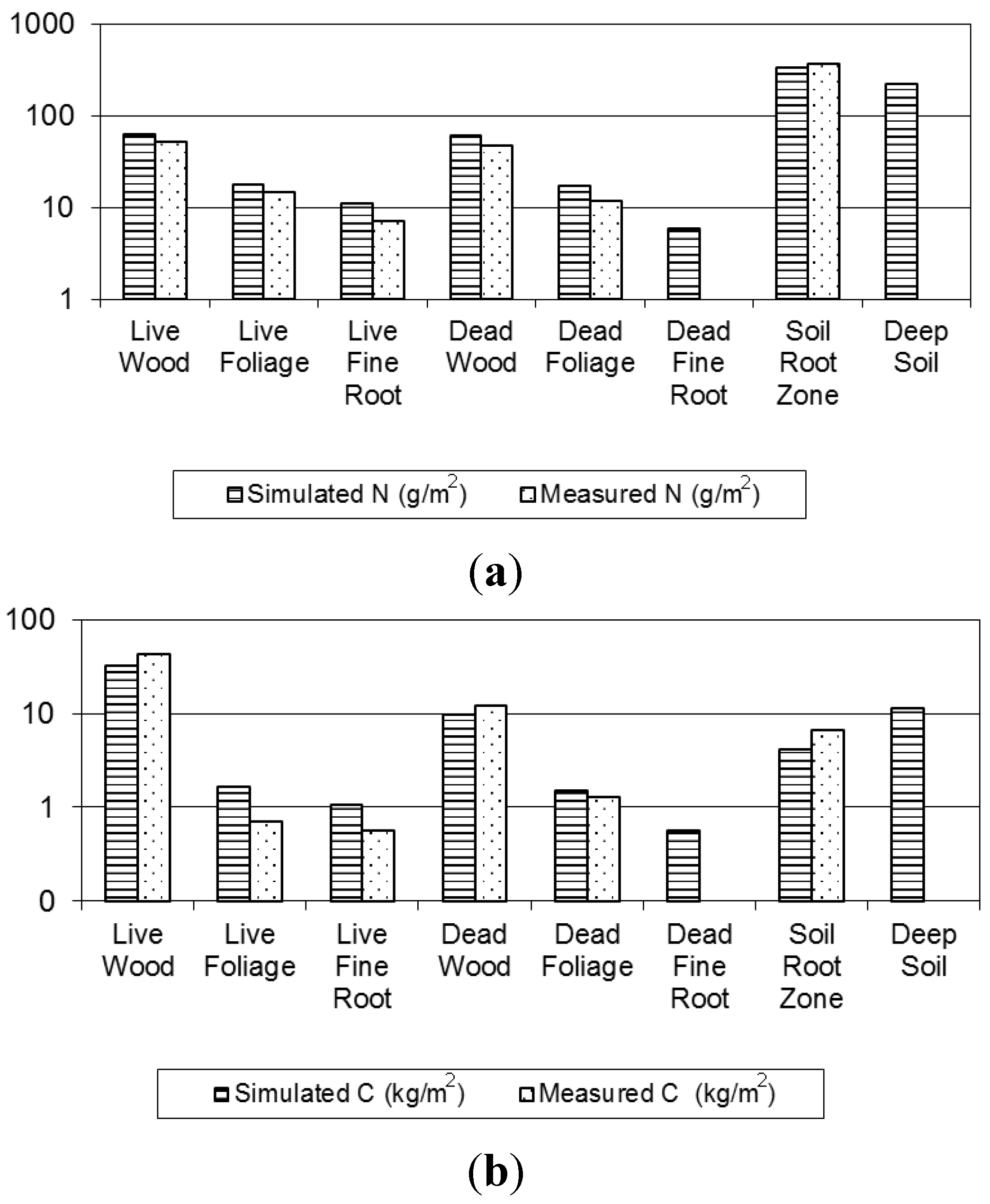
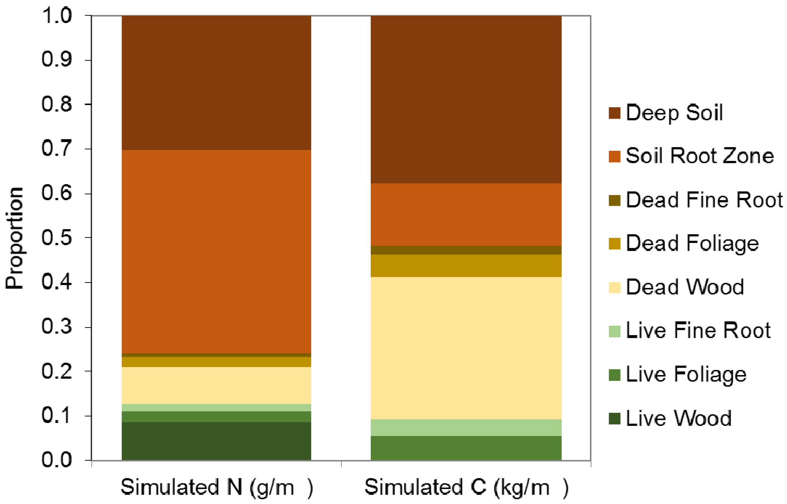
3.1.1. Evaluation of Budget Estimates of N and C Stocks

The average modeled results of the key nitrogen and carbon stocks are consistent with budget-based measurements that are available from WS10 [29], or have been taken from similar forested regions [41]. Key features of the results include a dominance of carbon storage in woody material (65% of total carbon storage) and nitrogen storage in soils (75% of total nitrogen storage) (Figure 2). Differences between the modeled values and the measurements were anticipated, particularly because the measured stocks were not necessarily binned in the same manner as the model description, and because we are comparing average model results representing 20 years of simulation to measurements that were developed to represent a full year, and in the case of the Wind River data [41], at different location. Direct comparisons between the available budget-based measurements and the model-based estimates (Figure 3 and Figure 4; Table 1) indicate that the model is able to capture the general magnitude of carbon and nitrogen storage, and also the differences between the key environmental compartments.

Figure 2. A comparison of simulated stocks of nitrogen (a) and carbon (b) against budget estimates from [29]. Note that estimates of observed C stocks (except for SOM, labelled above were originally derived by [28] and that we assumed the carbon content of dry mass was 50%. Additionally, we assumed that 50% of the category “Fallen foliage and fine woody litter” from [29] were dead foliage and that 50% were dead wood.

Figure 2. A comparison of simulated stocks of nitrogen (a) and carbon (b) against budget estimates from [29]. Note that estimates of observed C stocks (except for SOM, labelled above were originally derived by [28] and that we assumed the carbon content of dry mass was 50%. Additionally, we assumed that 50% of the category “Fallen foliage and fine woody litter” from [29] were dead foliage and that 50% were dead wood.

Figure 3. Measured versus modeled annual yearly storage of nitrogen and carbon. These data are also plotted in Figure 2. Each data point represents a different storage term, as outlined in Figure 2. A one to one line is included for reference.

Figure 3. Measured versus modeled annual yearly storage of nitrogen and carbon. These data are also plotted in Figure 2. Each data point represents a different storage term, as outlined in Figure 2. A one to one line is included for reference.

Figure 4. Model results for average annual storage of nitrogen and carbon. Results are normalized by the total sum of nitrogen and carbon.

Figure 4. Model results for average annual storage of nitrogen and carbon. Results are normalized by the total sum of nitrogen and carbon.

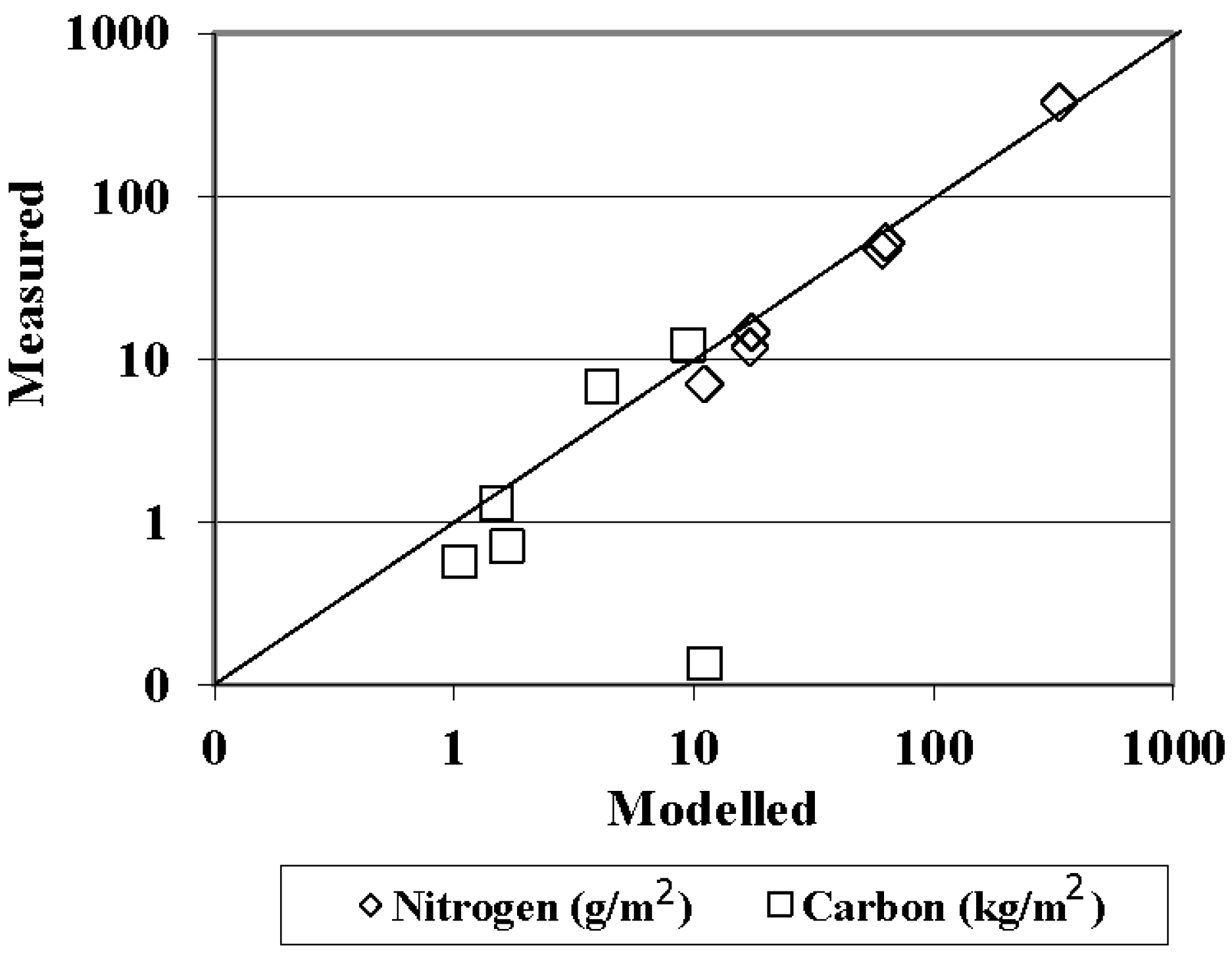
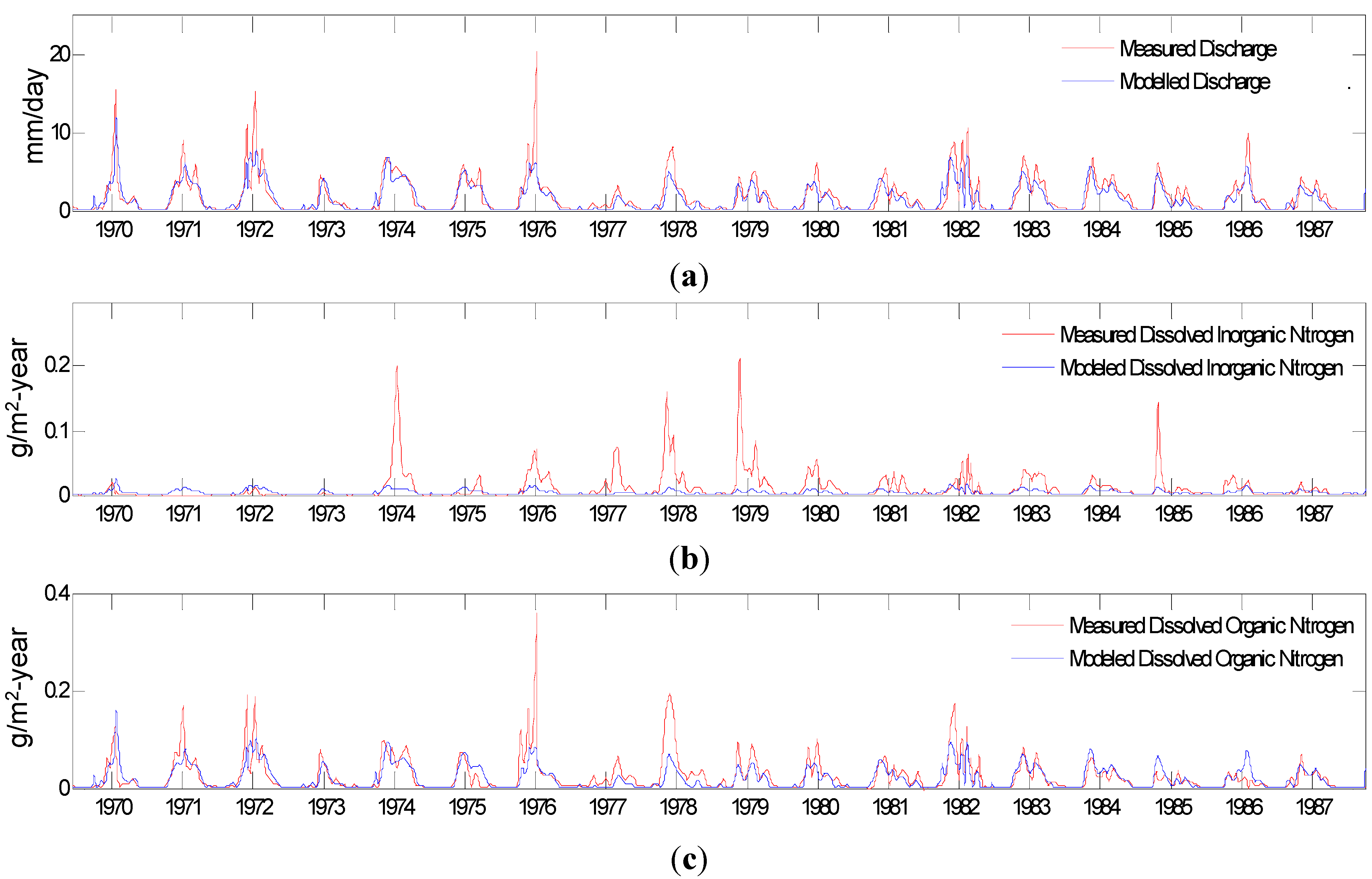
3.1.2. Model Evaluation against Observations

The long-term record, which includes stream water discharge, and DON and DIN export is rare, and provides an opportunity to constrain model operation. A comparison of the time series records to the modeled result is included in Figure 5 and demonstrates that model effectively captures the seasonal pattern that is outlined by the measured discharge and DON. For these variables, the modeled Nash Sutcliffe efficiency [42] values are 0.71 and 0.53 respectively. The efficiency for DIN is −0.12, which clearly indicates that the model does not capture the measured response. This apparent failure of the model is likely because we did not attempt to simulate impacts of the clear-cut harvest that occurred in 1975. The removal of the trees, and pre-treatment activity, led to elevated DIN export after the harvest. The effects on DIN of this disturbance have been explored by [43] and are clearly evident in the long-term record and has been attributed to reduced uptake of N by vegetation. It is worth noting that the calculated Nash-Sutcliffe for years prior to the management activity (1968 to 1973) is higher, 0.33, lending additional support to the suggestion.

Evaluation of against Budget Estimates of N and C Fluxes

Given that the model is capable of representing key long term output measurements of water, DIN and DON, and also the overall trends in storage, the next step is to evaluate the degree to which the model is working for the right reasons—this we accomplish through an evaluation of the internal rate terms. These rates include respiration, mobilization, immobilization, internal solute fluxes and the aquatic processes that follow from them. Here we return to the existing budget studies which provide a set of annual flux estimates which we utilize in calibration, and to better understand model function. Rate terms are broadly grouped into four categories representing carbon fluxes, the sources of nitrogen, SOM dynamics, and processes occurring in the aquatic environment. This division is not to suggest that these categories are independent of one another, but only to facilitate presentation of results. In all cases, we present continuous model results (Figure 6, Figure 7, Figure 8 and Figure 9) and in addition, time-integrated average yearly values (included in Figure 6, Figure 7, Figure 8 and Figure 9 and Table 9 and Table 10), which can be directly compared against yearly values from the budget studies.

Figure 5. Measured versus model time series for stream water discharge (a), dissolved inorganic nitrogen (b) and dissolved organic nitrogen (c). Nash-Sutcliffe efficiencies for discharge is 0.71, for DON is 0.53. For DIN the efficiency is −0.13, as discussed in the text, this is likely due to the clearcut that occurred in the watershed in the early 1970s. The model did not attempt to incorporate the effects of the management.

Figure 5. Measured versus model time series for stream water discharge (a), dissolved inorganic nitrogen (b) and dissolved organic nitrogen (c). Nash-Sutcliffe efficiencies for discharge is 0.71, for DON is 0.53. For DIN the efficiency is −0.13, as discussed in the text, this is likely due to the clearcut that occurred in the watershed in the early 1970s. The model did not attempt to incorporate the effects of the management.

Table 9. Comparison of modeled pool sizes (averaged over the 20 year simulation period) against measured values as reported in (a) [29] from WS10 and from (b) [41] from Wind River, WA. We assumed a carbon content of 50% to estimate C from the dry mass reported in [29]. The standard deviation of the modeled values is included in parenthesis.

Ecosystem Component		C (kg/m2)			N (g/m2)		CN
		a	b	Model	a	Model	a	Model
Vegetation	Wood	42.29	37.87	31.77 (0.04)	52.17	63.3 (0.11)	810.63	501.57
	Foliage	0.69	0.94	2.17 (0.04)	14.44	18.2 (0.38)	48.13	119.20
	Fine Roots	0.06	0.36	1.12 (0.04)	0.69	11.7 (0.16)	80.65	96.34
Detritus	Wood	13.31	9.87	9.54 (0.05)	47.1	61.1 (0.58)	282.59	156.05
	Foliage	1.28	1.78	2.01 (0.02)	11.76	18.1 (0.15)	108.84	110.73
	Fine Roots		0.48	0.593 (0.01)		6.4 (0.11)		93.06
Soil	Root Zone	6.65	9.3	4.28 (0.06)	372.4	338.5 (4.23)	17.88	12.65
	Deep Soil			12.80 (0.33)		220.5 (5.39)		58.07

Table 9. Comparison of modeled pool sizes (averaged over the 20 year simulation period) against measured values as reported in (a) [29] from WS10 and from (b) [41] from Wind River, WA. We assumed a carbon content of 50% to estimate C from the dry mass reported in [29]. The standard deviation of the modeled values is included in parenthesis.

Ecosystem Component		C (kg/m2)			N (g/m2)		CN
		a	b	Model	a	Model	a	Model
Vegetation	Wood	42.29	37.87	31.77 (0.04)	52.17	63.3 (0.11)	810.63	501.57
	Foliage	0.69	0.94	2.17 (0.04)	14.44	18.2 (0.38)	48.13	119.20
	Fine Roots	0.06	0.36	1.12 (0.04)	0.69	11.7 (0.16)	80.65	96.34
Detritus	Wood	13.31	9.87	9.54 (0.05)	47.1	61.1 (0.58)	282.59	156.05
	Foliage	1.28	1.78	2.01 (0.02)	11.76	18.1 (0.15)	108.84	110.73
	Fine Roots		0.48	0.593 (0.01)		6.4 (0.11)		93.06
Soil	Root Zone	6.65	9.3	4.28 (0.06)	372.4	338.5 (4.23)	17.88	12.65
	Deep Soil			12.80 (0.33)		220.5 (5.39)		58.07

Figure 6. Key modeled rate terms associated with carbon cycling. (a) The plot represents the modeled time series, as indicated in the legend, across the 20 year simulation time frame. These data are summarized and presented as a box and whisker plot (b). Note that the y axis is log transformed in the upper plot, but is linear in the lower plot. The combination is provided to more clearly outline the range in variation.

Figure 6. Key modeled rate terms associated with carbon cycling. (a) The plot represents the modeled time series, as indicated in the legend, across the 20 year simulation time frame. These data are summarized and presented as a box and whisker plot (b). Note that the y axis is log transformed in the upper plot, but is linear in the lower plot. The combination is provided to more clearly outline the range in variation.

Figure 7. Key modeled rate terms associated with the input of nitrogen into the system. (a) The plot represents the modeled time series, as indicated in the legend, across the 20 year simulation time frame. These data are summarized and presented as a box and whisker plot (b). Note that the y axis is log transformed in the upper plot, but is linear in the lower plot.

Figure 7. Key modeled rate terms associated with the input of nitrogen into the system. (a) The plot represents the modeled time series, as indicated in the legend, across the 20 year simulation time frame. These data are summarized and presented as a box and whisker plot (b). Note that the y axis is log transformed in the upper plot, but is linear in the lower plot.

Figure 8. Key modeled rate terms associated with root zone SOM. (a) The plot represents the modeled time series, as indicated in the legend, across the 20 year simulation time frame. These data are summarized and presented as a box and whisker plot (b). Note that the y axis is log transformed in the upper plot, but is linear in the lower plot.

Figure 8. Key modeled rate terms associated with root zone SOM. (a) The plot represents the modeled time series, as indicated in the legend, across the 20 year simulation time frame. These data are summarized and presented as a box and whisker plot (b). Note that the y axis is log transformed in the upper plot, but is linear in the lower plot.

Figure 9. Key modeled rate terms associated with SOM processing occurring below the root zone. (a) The plot represents the modeled time series, as indicated in the legend, across the 20 year simulation time frame. These data are summarized and presented as a box and whisker plot (b). Note that the y axis is log transformed in the upper plot, but is linear in the lower plot.

Figure 9. Key modeled rate terms associated with SOM processing occurring below the root zone. (a) The plot represents the modeled time series, as indicated in the legend, across the 20 year simulation time frame. These data are summarized and presented as a box and whisker plot (b). Note that the y axis is log transformed in the upper plot, but is linear in the lower plot.

Table 10. Simulated average annual rates defining the carbon model. The rates in bold are summaries across each of the individual compartments.

Rate	g/m2-year
Gross primary production	935.28
Growth wood	44.34
Growth foliage	177.34
Growth fine roots	217.96
Total growth (NPP)	439.63
Mortality wood	32.56
Mortality foliage	176.62
Mortality fine roots	217.35
Total mortality	426.53
Decomposition from wood	4.37
Decomposition from foliage	127.54
Decomposition from fine roots	185.66
Total decomposition	672.16
Respiration from wood	39.35
Respiration from foliage	0.01
Respiration from fine roots	32.76
Respiration from SOM RZ	173.98
Respiration from SOM BRZ	44.16
Respiration heterotrophic	332.78
Respiration Autotrophic	495.70
Total respiration	828.48
DOC Production RZ	17.4
DOC Production BRZ	4.42
Total DOC production	21.82

Table 10. Simulated average annual rates defining the carbon model. The rates in bold are summaries across each of the individual compartments.

Rate	g/m2-year
Gross primary production	935.28
Growth wood	44.34
Growth foliage	177.34
Growth fine roots	217.96
Total growth (NPP)	439.63
Mortality wood	32.56
Mortality foliage	176.62
Mortality fine roots	217.35
Total mortality	426.53
Decomposition from wood	4.37
Decomposition from foliage	127.54
Decomposition from fine roots	185.66
Total decomposition	672.16
Respiration from wood	39.35
Respiration from foliage	0.01
Respiration from fine roots	32.76
Respiration from SOM RZ	173.98
Respiration from SOM BRZ	44.16
Respiration heterotrophic	332.78
Respiration Autotrophic	495.70
Total respiration	828.48
DOC Production RZ	17.4
DOC Production BRZ	4.42
Total DOC production	21.82

Table 11. Simulated average annual rates defining the nitrogen model. The rates in bold are summaries across each of the individual compartments.

Rate	g/m2-year
DON_Deposition	0.04
DIN_Deposition	0.03
Total deposition	0.08
Symbiotic fixation allocated to wood	0
Symbiotic fixation allocated to foliage	0
Symbiotic fixation allocated to roots	0.43
Total symbiotic fixation	0.43
Uptake allocated to wood	0.04
Uptake allocated to foliage	1.79
Uptake allocated to roots	1.87
Total uptake	3.70
Mortality wood	0.06
Mortality foliage (litterfall)	1.81
Mortality roots	2.33
Total turnover	4.21
Asymbiotic fixation allocated to wood	0.08
Asymbiotic fixation allocated to foliage	0.08
Asymbiotic fixation allocated to roots	0.076
Total asymbiotic fixation	0.22
Decomposition of wood	0.27
Decomposition of foliage	1.93
Decomposition of roots	2.42
Total decomposition	4.64
DON mobilization (RZ)	2.58
DIN mobilization (RZ)	2.58
DIN Immobilization (RZ)	1.19
DON breakdown to DIN (RZ)	2.28
DON transport in RZ	0.34
DIN transport in RZ	0.00
Denitrification RZ	0.00
DON mobilization (BRZ)	1.92
DIN mobilization (BRZ)	1.17
DIN Immobilization (BRZ)	2.67
DON breakdown to DIN (BRZ)	2.23
DON transport in BRZ	0.62
DIN transport in BRZ	0.020
Denitrification BRZ	0.01
Particulate input to aquatic	1.88
DON mobilization	0.00
DIN immobilization	0.00
DIN mobilization	0.00
Denitrification from aquatic	0.00
DIN export	0.00
DON export	0.02
Particulate export	0.02

Table 11. Simulated average annual rates defining the nitrogen model. The rates in bold are summaries across each of the individual compartments.

Rate	g/m2-year
DON_Deposition	0.04
DIN_Deposition	0.03
Total deposition	0.08
Symbiotic fixation allocated to wood	0
Symbiotic fixation allocated to foliage	0
Symbiotic fixation allocated to roots	0.43
Total symbiotic fixation	0.43
Uptake allocated to wood	0.04
Uptake allocated to foliage	1.79
Uptake allocated to roots	1.87
Total uptake	3.70
Mortality wood	0.06
Mortality foliage (litterfall)	1.81
Mortality roots	2.33
Total turnover	4.21
Asymbiotic fixation allocated to wood	0.08
Asymbiotic fixation allocated to foliage	0.08
Asymbiotic fixation allocated to roots	0.076
Total asymbiotic fixation	0.22
Decomposition of wood	0.27
Decomposition of foliage	1.93
Decomposition of roots	2.42
Total decomposition	4.64
DON mobilization (RZ)	2.58
DIN mobilization (RZ)	2.58
DIN Immobilization (RZ)	1.19
DON breakdown to DIN (RZ)	2.28
DON transport in RZ	0.34
DIN transport in RZ	0.00
Denitrification RZ	0.00
DON mobilization (BRZ)	1.92
DIN mobilization (BRZ)	1.17
DIN Immobilization (BRZ)	2.67
DON breakdown to DIN (BRZ)	2.23
DON transport in BRZ	0.62
DIN transport in BRZ	0.020
Denitrification BRZ	0.01
Particulate input to aquatic	1.88
DON mobilization	0.00
DIN immobilization	0.00
DIN mobilization	0.00
Denitrification from aquatic	0.00
DIN export	0.00
DON export	0.02
Particulate export	0.02

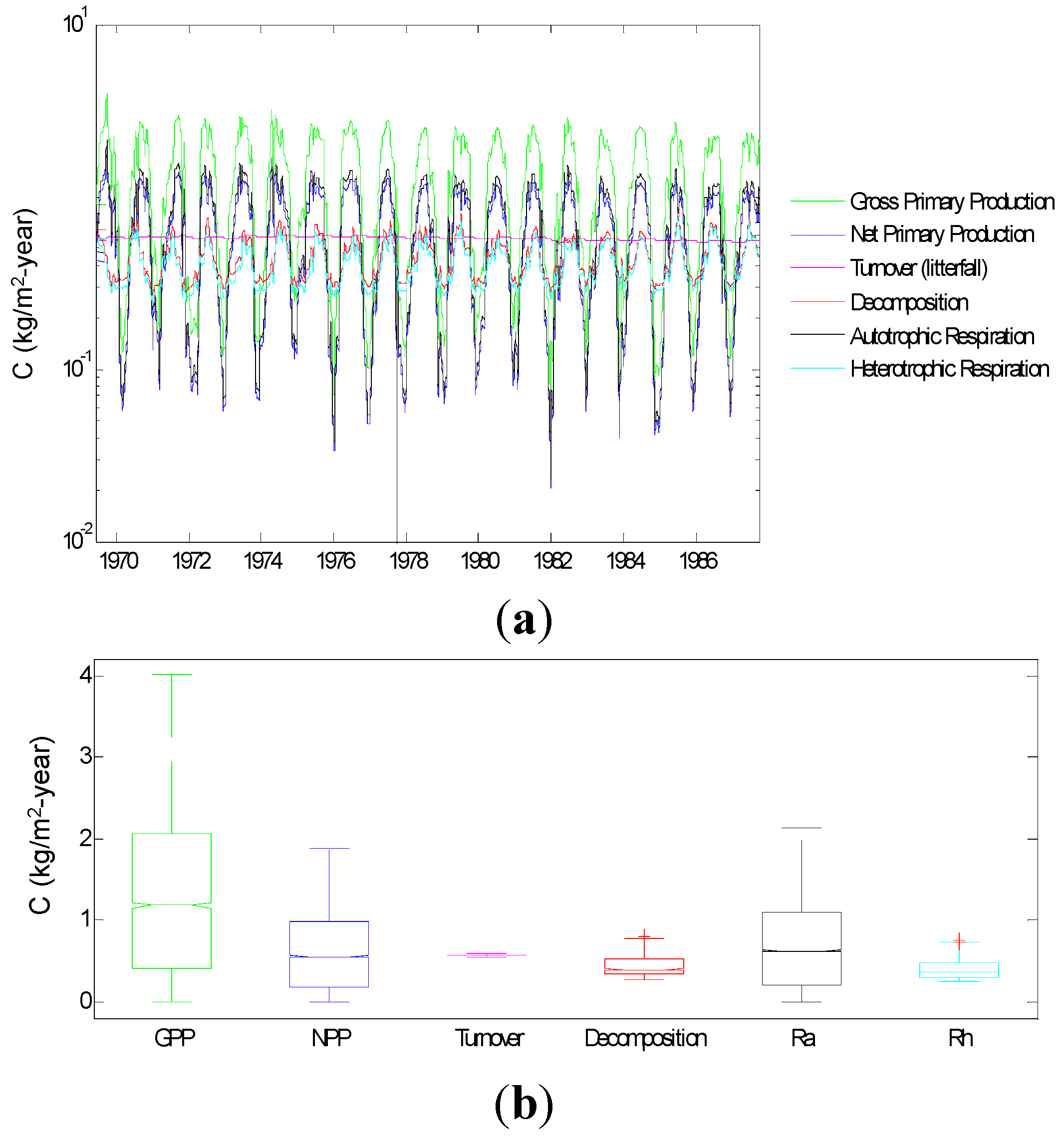
3.1.3. Carbon Fluxes

The key rate terms capturing carbon dynamics are gross and net primary production, turnover (including mortality and litterfall), and both autotrophic and heterotrophic respiration. Model results for each rate term were integrated over the 20 year simulation period, and the yearly average over that time period is presented in Table 9. The average yearly gross primary productivity is estimated as 1.4 kg/m²-year, with the daily rates ranging from nearly 0 kg/m²-year (periodically during the winter period) to over 3 kg/m²-year (Figure 6). The average yearly rate is somewhat lower than the range of 1.4 to 3.3 kg/m²-year estimated by [41] for a similar old growth forest, and within the range of 1.08–1.92 kg/m²-year estimated using remote sensing techniques across a Douglas-fir western hemlock forest on Vancouver Island, Canada by [44]. The simulated values are considerably lower than the 11.1–21.7 kg/m²-year estimated by [28] at HJA in 1970, and different respiration estimates explain the discrepancy. We assumed a respiration value of 47% of GPP, a heuristic model generated as part of the collaborative model development process. The older budgets of [28] resulted in respiration values of 92%–94% of GPP. Given the assumption that Ra is 47% of GPP, the yearly average NPP from the model is 0.60 kg/m²-year. This value is similar to other estimates of NPP reported at other similar sites, for example [41] estimated a range of NPP from 0.45–0.741 kg/m²-year at similar location in Washington State, [28] estimated a range from 0.41 to 0.66 kg/m²-year at HJA and [45] used a model to estimate a stable value of 0.50 kg/m²-year at HJA. Our model estimates are within the wide range of variation possible for NPP. The constant fraction model to estimate R_a explains the similarity in the time series representing NPP and R_a in Figure 6. Turnover is treated as a first order model which does not include any outside dependence (for example air temperature, soil water content, etc.). This is reflected in the low temporal variation displayed for the turnover rate. The modeled value of average yearly turnover (0.572 kg/m²-year) is similar to that measured by [41] which ranged from 0.370 to 0.690 kg/m²-year. Modeled heterotrophic respiration (R_h) is defined to include the production of CO₂ and DOC from litter and soils. The average yearly value of 0.397 kg/m²-year is of within the range of 0.341 to 0.509 kg/m²-year estimated by [43].

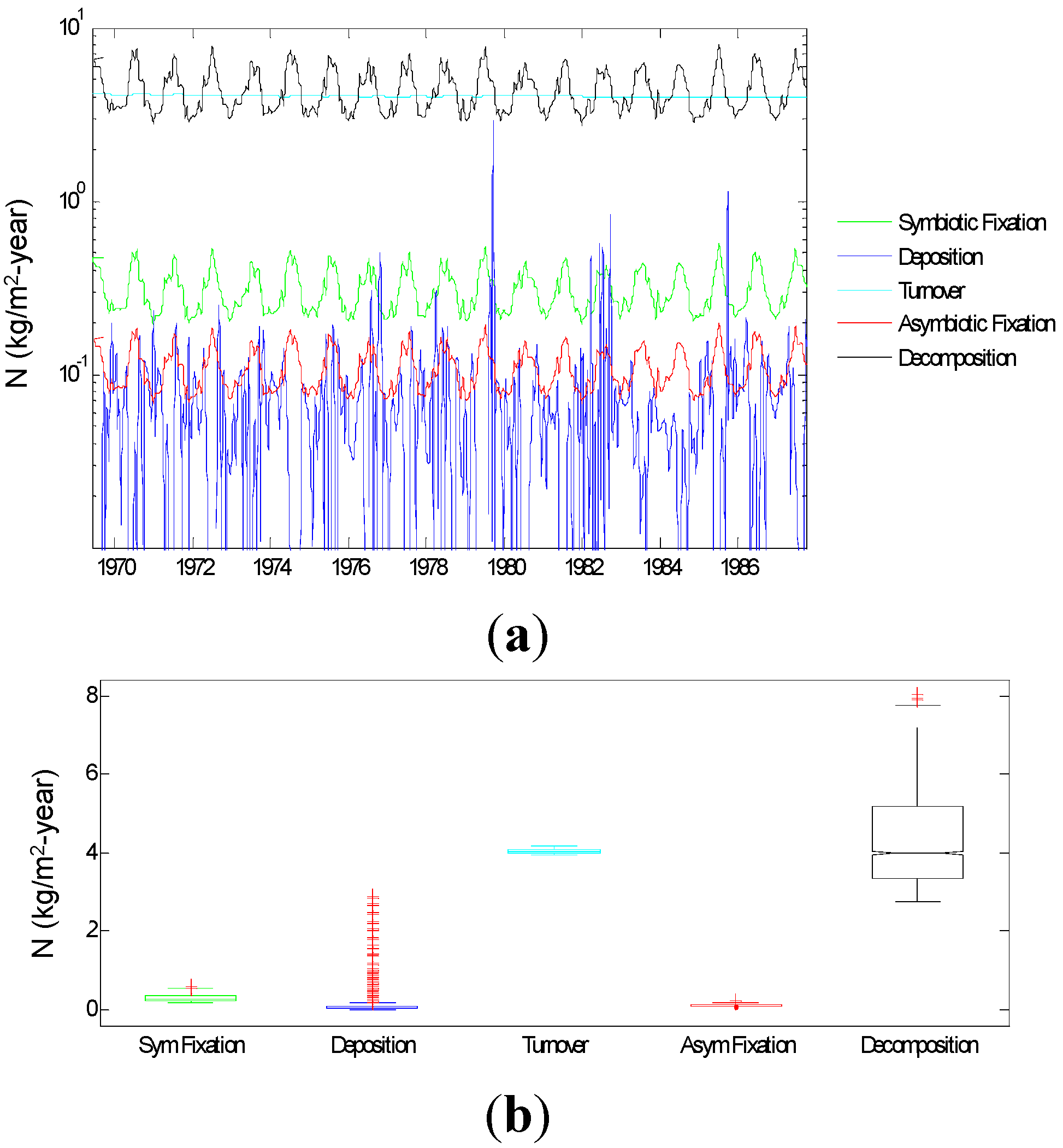
3.1.4. Input of N to SOM

External inputs of N include deposition, and both symbiotic and asymbiotic fixation. Internal inputs of N to SOM include both mortality/litterfall and decomposition. Decomposition and turnover rates—internal recycling—are simulated to be at least an order of magnitude larger than the external rates (Figure 7). The external rates of deposition (which include both DIN and DON) are simply measurements, and the fixation rate terms have been calibrated to mimic the few estimates that are available for these sites. Symbiotic respiration in WS10 have been estimated to be 0.280 g/m²-year [29], which is of a similar order to our average yearly modeled estimate of 0.305 g/m²-year. The modeled estimate of asymbiotic fixation is 0.107 g/m²-year. Actual asymbiotic fixation rates of, on average, 0.45 umol/g/day have been estimated for the tree species which dominated W10 prior to the clearcut in 1975 (Psuedotsuga menziesii) [46]. Given the model’s average annual litter estimate of 43.55 kg/m², this measured fixation rate is equivalent to 0.100 g/m²-year, in close agreement with the model rate. A complete listing of time integrated average nitrogen fluxes is included in Table 10.

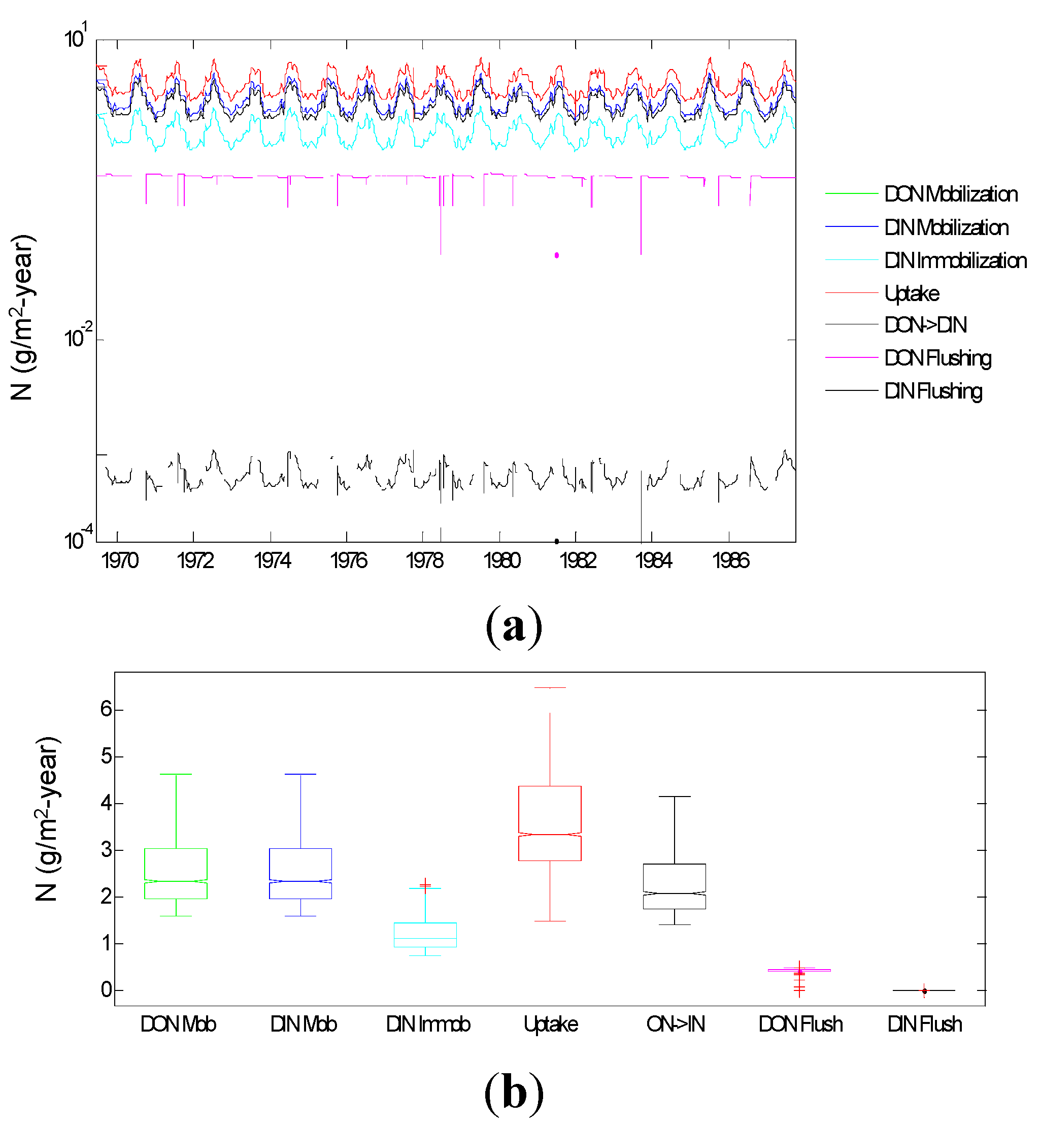
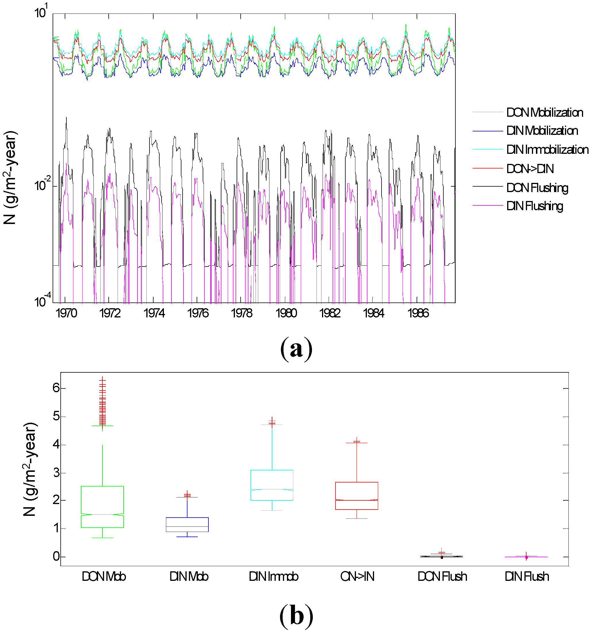
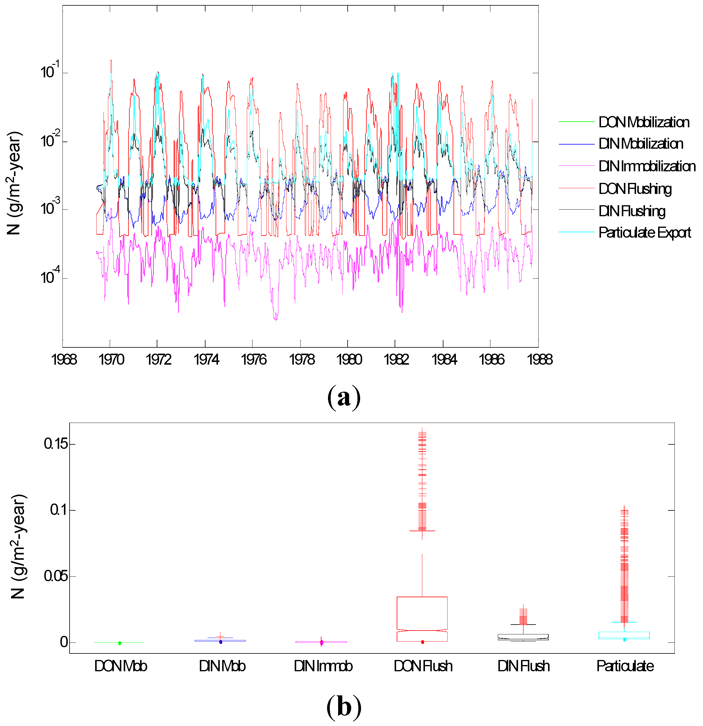
3.1.5. Root Zone N Dynamics

The dynamics of nitrogen in the root zone are defined primarily by a series of seven rate terms, including the mobilization and flushing of DON and DIN, the immobilization and uptake by vegetation of DIN, and the breakdown of DON to produce DIN, which occurs through respiration processes. There is also potential for denitrification as a pathway of loss, however given the well aerated nature of soils in WS10, we assume that denitrification does not occur in the root zone. These terms are outlined in Figure 8, as both time series and box plots. These results indicate a net mobilization (mineralization) of inorganic nitrogen of 2.51 g/m²-year, and that mobilization of DON is 2.51 g/m²-year. The values are equivalent because, without additional data, we simply assume that total nitrogen mobilization was proportional to respiration and that the product was half organic and half inorganic nitrogen. Mobilized DON is continuously decomposed to further add to the DIN pool, most of which is utilized through plant uptake. The average yearly uptake rate is 3.62 g/m²-year, similar to the 2.29 g/m²-year estimated by [13]. The rate of flushing for DON (0.337 g/m²-year) is considerably larger than for DIN, which was effectively 0 for our simulations. This result is consistent with the well-established high N retention capacity of these watersheds. The rates of flushing periodically fall to zero, indicated as breaks in the time series in Figure 8. This occurs when amounts of DIN or DON are not sufficient to support all of the simulated loss pathways.

3.1.6. N Dynamics below the Root Zone

Below root zone dynamics are similar to those simulated in the root zone, with flushing rates of both DON and DIN significantly lower than the rates of internal recycling (Figure 9). However, flushing rates of DON are larger than from within the rooting zone (467.7 mg/m²-year root zone compared to 283.6 mg/m²-year below the root zone), while flushing of DIN is somewhat higher from below the rooting zone (0.36 mg/m²-year root zone compared to 23.61 mg/m²-year below the root zone) primarily because vegetation is no longer able to mediate the flux of DIN from below the rooting zone. The model results indicate that the region below the root zone is a moderate nitrogen sink, with a net mobilization value of −99.40 mg/m²-year. No measurements exist within this region of the watershed, and Figure 9 therefore represents only one possible result which is consistent with both simulated inputs from the root zone, and more importantly, measured outputs of water and dissolved nitrogen from the catchment.

3.1.7. Aquatic Environment

Figure 10. Key modeled rate terms associated with the aquatic environment. (a) The plot represents the modeled time series, as indicated in the legend, across the 20 year simulation time frame. These data are summarized and presented as a box and whisker plot (b). Note that the y axis in log transformed in the upper plot, but is linear in the lower plot.

Figure 10. Key modeled rate terms associated with the aquatic environment. (a) The plot represents the modeled time series, as indicated in the legend, across the 20 year simulation time frame. These data are summarized and presented as a box and whisker plot (b). Note that the y axis in log transformed in the upper plot, but is linear in the lower plot.

The discussion of the aquatic environment focuses on mobilization and immobilization of N, as well as flushing. Particulate export of N dominates the model results in the aquatic region, with simulated values of 1.73 g/m²-year. A value of 2.53 g/m²-year was estimated by [30] for a particular year. The next largest rate term in the aquatic environment, DON export, is 0.024 g/m²-year, and because of the approximately two orders of magnitude difference, particulate export has not been included in Figure 10. Results indicate net immobilization of DIN (3.42 mg/m²-year) occurs in the aquatic region, consistent with [47] for a somewhat larger stream in HJA. The dynamic model results also indicate, however, that during the growing season, the instream biomass can function as a source of N, primarily because DIN limitation caps the growth rate, yet DIN mobilization is treated with first order dependence on the aquatic biomass, and so proceeds at a relatively higher rate during periods of low DIN availability (Figure 10). Nevertheless, even excluding simulated particulate export, model results indicate that more nitrogen is lost from the stream environment on a yearly basis in dissolved forms (24.8 mg/m²-year) that is retained within it by the aquatic biomass (3.42 mg/m²-year).

3.2. Discussion

HJA-N was constructed in an effort to explore relationships between biotic and abiotic processes in the retention and release of nitrogen from small watersheds. An elementary, yet key, finding is that the model can be parameterized so as to produce results that are consistent with a wide range of measurements from WS10 or from similar sites. This result is a prerequisite for any further analysis. Having established consistency with available measurements, the model results can be further evaluated to provide a number of intriguing insights into how watershed components interact over seasonal timescales to recycle nitrogen. The important contribution of the model is that it allows us to quantify the seasonal variability of rate terms, greatly extending the budget based estimates of storage and fluxes which comprise a significant amount of available measurements [28,29,30,41].

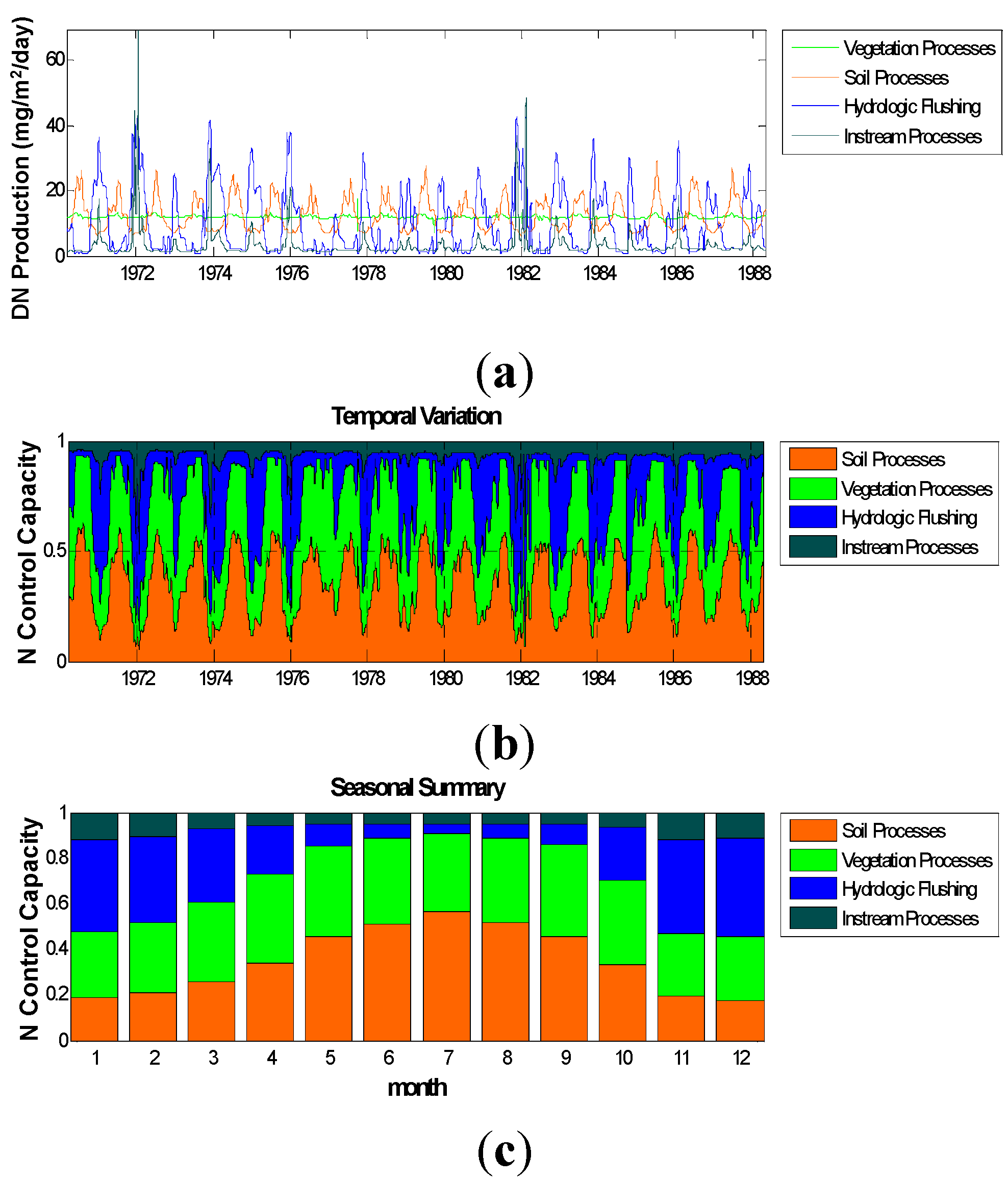
3.2.1. Relative Importance of Various System Components

A key theme of this research is the development of quantitative, internally consistent estimates of the relative roles of watershed components in the retention and release of nitrogen over seasonal timescales. The overall goal is the exploration of the temporally varying relationship between these components—vegetation, soils, hydrology, and the aquatic environment—in regulating the release of nitrogen from the system. In the hydrologic literature, much work in this direction has focused on the concept of hydrologic flushing [48]. At the same time, it is often assumed in both the soils and forest ecology literature (e.g., [49]) that the temporal variation in net mobilization is ultimately responsible for the availability of any nitrogen that might be flushed out of the system by the hydrology. This mobilization potential is particularly relevant in regions, like the PNW, where atmospheric deposition remains low. All the while, the role of the stream channel, as well as the riparian vegetation [47] in immobilizing significant amounts available nitrogen from the aquatic system, and hence modifying cross-weir export measurements, frequently remains unnoticed in catchment studies. And perhaps even more importantly in systems where nitrogen is strongly retained, the particulate export of dissolved organic nitrogen, over which the aquatic system exerts significant control, is often of a similar magnitude, if not considerably larger, than the export of dissolved nitrogen [30].

Our modeling work indicates that hydrologically-mediated fluxes are much smaller in magnitude (DON + DIN export of 22.1 mg/m²-year) than the mobilization fluxes that occur within the vegetation (747.7 mg/m²-year N mobilization, decomposition-uptake) or within the root zone SOM (3838.3 mg/m²-year) N mobilization. This finding is consistent with the wide variety of observational work at HJA [29] and has also been demonstrated at other forested watersheds [43]. However, the hydrologically-mediated fluxes are larger in magnitude to the immobilization potential of the aquatic environment (3.42 mg/m²-year) (Figure 6, Figure 7, Figure 8, Figure 9 and Figure 10). These observations provide a useful means of understanding the system and ranking system components as to their role in the regulation of nitrogen cycling. In addition, the model results provide data that can be evaluated at finer seasonal time scales.

Control Capacity

We interpret the N control capacity ratio as the degree of control that each system components exerts on the release dynamics of nitrogen cycling within the model domain (Figure 11). There is, of course, a degree of subjectivity in the definitions, nonetheless evaluating the results in this fashion provides a unique mechanism to evaluate the relative importance of components, and how this degree of control varies with time. These kinds of analyses are available only through the use of the continuously varying results, which are not typically measured over long periods, providing significant further utility in the application and development of conceptual numerical simulation.

Figure 11. The nitrogen control capacity. (a) The plot outlines the summed rate terms which are used to estimate the control capacity of the watershed components as indicated in the legend. These four time series correspond directly to Equations (1)–(4); (b) The plot represents the control capacity, where the time series from the upper plot have been normalized by the total rate of nitrogen movement. (c) The plot represents the monthly averages of the control capacity, again including comparisons of the four different watershed components.

Figure 11. The nitrogen control capacity. (a) The plot outlines the summed rate terms which are used to estimate the control capacity of the watershed components as indicated in the legend. These four time series correspond directly to Equations (1)–(4); (b) The plot represents the control capacity, where the time series from the upper plot have been normalized by the total rate of nitrogen movement. (c) The plot represents the monthly averages of the control capacity, again including comparisons of the four different watershed components.

As expected given the well-established capacity of these types of watersheds to retain N, vegetation and soils exert a primary control on N dynamics. Hydrologic flushing of nitrogen is well-represented during the winter period, though even during periods of elevated N export and flushing, vegetation and soils still represent important controls (Figure 11). The explanation behind the result is clear—the Mediterranean climate in the Pacific Northwest results in significant winter moisture, which produces increased soil moisture, higher soil water flux, and larger stream discharge than seen during the dry summer period. In addition, the lower temperatures that dominate during the winter period suppress primary production and SOM dynamics. During the growing season, however, hydrologic flushing moves into the background, while control capacity of other components increases. This change in control is most evident in June–August, when mobilization rates tend to increase and flushing rates decrease. SOM contributes a larger portion of available nitrogen than the vegetation during this period of time, and this is primarily because uptake increases and the vegetation acts as a stronger sink of N that SOM during the summer period. This difference is in part a reflection of our lumping of litter and live biomass in our definition of control capacity. Particulate flushing of nitrogen mimics hydrologic flushing because of increased mobilization of aquatic biomass during the wet season, but the signal is muted when compared to hydrologic flushing. The lower seasonal variability develops at least in part because particulate inputs are derived directly from the litterfall/mortality model which did not include seasonal effects.

These results lend credence to the idea that understanding the dynamics of nitrogen, carbon, and water in ecosystems requires a multidisciplinary approach [39]. This approach certainly includes attention to flushing behavior, but the level of attention given to flushing must be on par with that given to production of available nitrogen, which may be dissolved or in particulate forms. Furthermore, the seasonality of the system imposes a series of constraints that result in predictable temporal variation in the activity of different system components. This variation is difficult to approach through standard field-based budget techniques; however numerical modeling can be used to extend budget results to provide a clearer picture of the seasonality.

3.2.2. Limitations of the Modeling Framework

The model framework and analyses presented here represent a step in our evolving understanding of how small catchments at HJA function. There are, however, a number of limitations to this work. The modeling focuses on an approximately monthly time series of input output data, which provides insight into seasonal dynamics. However, this time step is too coarse to understand the finer time dynamics that are often the focus of experimentalists working within the wide variety of contributing disciplines. At the same time, it may be too coarse to understand the longer term evolution of catchments, both in terms of nitrogen availability and changing climate. We envision significant potential to redevelop these modeling ideas to correspond to these different timescales—but the model as presented herein is not suited to either. Similarly, while we included a simple model of instream particulate retention and release, extreme events are not included. These events include for example large storms, mass movement, and fire, and in terms of nitrogen control, it is clear that over long time scales, these are at least as significant as the biotic controls and flushing that we explored here. These limitations simply mean that interpreting the results outside of the timeframe over which the model was run is not possible.

The model outlined here includes a variety of parameters that cannot be measured directly. For example to separate net nitrogen mineralization into gross mineralization and gross immobilization requires a set of measurements that are very difficult to perform at point scales [50]. And further, the relationship between these point scale observations for catchment level simulations is not well-established. Yet competition between vegetation and microbes is a key feature of nitrogen cycling [51], and microbial immobilization and mobilization, as well as plant uptake must be included in a model designed to explore the effects of this competition. The parameters involved in this portion of the model (and others) are developed based solely upon educated guesses, and calibration procedures relying upon evaluation of the resulting rate terms. In the case of models developed for predictive purposes, simpler tends to be more effective, and incorporating net mineralization, which can be more readily measured, would make more sense. Nonetheless, while some of our decisions clearly reduce the predictive capability of the model through increased parameter uncertainty, the more complete structural definition provides a framework to outline both what is known, and what hypothesized about how these catchments function with respect to N cycling.

Some of the most interesting aspects of watershed nitrogen work to emerge in the last two decades involve the role of spatially disaggregated watershed components in the processing of key stocks. This spatial dependence is evident throughout the literature, including terrestrial biogeochemistry, aquatic processes, catchment hydrologic processes, hyporheic zone interactions, climate science, and forest ecology. As constructed, HJA-N does include some quasi spatial distribution, but this distribution simply separates the upslope processes from the near stream processes. From both a biotic and abiotic standpoint, this is a large simplification. An important next step is the incorporation of similar mass balance equations within a spatially-distributed model that would better allow for the incorporation of key differences in spatial distribution of ecosystem processes.

Lastly, a more complete evaluation of the model is needed to provide further guidance in terms of parameter sensitivity and associated model uncertainty. Sensitivity analyses also have the potential to provide insight into the degree of understanding we have regarding different model components, and as such assist in the prioritization of experimental studies designed to improve the both the general understanding of the system, and the predictive capability of the model.

4. Conclusions

The primary goal behind the development of HJA-N was to distill knowledge from a variety of disciplinary scientists, including key observational datasets, to succinctly describe N dynamics in WS10 at HJA. In doing so, we have produced a temporally dynamic simulation, which produces results that are consistent with existing water, N, and C budgets. One of the motivations was to construct a tool that could be used to quantify the relative roles of vegetation, hydrology, soils and SOM, and the near stream zone in controlling the release of N in retentive regions like HJA. The key finding is that each of the different catchment elements plays a significant role in the retention of N, and that those roles vary seasonally. While in and of itself, this is not entirely surprising, the ability to quantify those contributions provides a useful means to more fully understand how the catchment functions with respect to N dynamics.

References

1. Galloway, J.N.; Dentener, F.J.; Capone, D.G.; Boyer, E.W.; Howarth, R.W.; Seitzinger, S.P.; Asner, G.P.; Cleveland, C.C.; Green, P.A.; Holland, E.A.; et al. Nitrogen cycles: Past, present, and future. Biogeochemistry 2004, 70, 153–226. [Google Scholar]
2. Matson, P.; Lohse, K.A.; Hall, S.J. The globalization of nitrogen deposition: Consequences for terrestrial ecosystems. AMBIO J. Hum. Environ. 2002, 31, 113–119. [Google Scholar] [CrossRef]
3. Van Breemen, N.; Boyer, E.W.; Goodale, C.L.; Jaworski, N.A.; Paustian, K.; Seitzinger, S.P.; Lajtha, K.; Mayer, B.; van Dam, D.; Howarth, R.W.; et al. Where did all the nitrogen go? Fate of nitrogen inputs to large watersheds in the northeastern USA. Biogeochemistry 2002, 57, 267–293. [Google Scholar] [CrossRef]
4. Perakis, S.S.; Sinkhorn, E.R. Biogeochemistry of a temperate forest nitrogen gradient. Ecology 2011, 92, 1481–1491. [Google Scholar] [CrossRef] [PubMed]
5. Aber, J.D.; Nadelhoffer, K.J.; Steudler, P.; Melillo, J.M. Nitrogen saturation in northern forest ecosystems. BioScience 1989, 39, 378–286. [Google Scholar] [CrossRef]
6. Stoddard, J.L. Long-term changes in watershed retention of nitrogen. Its causes and aquatic consequences. In Environmental Chemistry of Lakes and Reservoirs, Edition: Advances in Chemistry Series, Edition Advances in Chemistry Series; American Chemical Society: Washington, DC, USA, 1994; Volume 237, pp. 223–284. [Google Scholar]
7. Meixner, T.; Fenn, M. Biogeochemical budgets in a Mediterranean catchment with high rates of atmospheric N deposition—Importance of scale and temporal asynchrony. Biogeochemistry 2004, 70, 331–356. [Google Scholar] [CrossRef]
8. Curtis, C.J.; Evans, C.D.; Goodale, C.L.; Heaton, T.H. What have stable isotope studies revealed about the nature and mechanisms of N saturation and nitrate leaching from semi-natural catchments? Ecosystems 2011, 14, 1021–1037. [Google Scholar] [CrossRef]
9. Whitehead, P.G.; Lapworth, D.J.; Skeffington, R.A.; Wade, A. Excess nitrogen leaching and C/N decline in the Tillingbourne catchment, southern England: INCA process modelling for current and historic time series. Hydrol. Earth Syst. Sci. 2002, 6, 455–466. [Google Scholar] [CrossRef]
10. Cosby, B.J.; Ferrier, R.C.; Jenkins, A.; Emmett, B.A.; Wright, R.F.; Tietema, A. Modelling the ecosystem effects of nitrogen deposition: Model of Ecosystem Retention and Loss of Inorganic Nitrogen (MERLIN). Hydrol. Earth Syst. Sci. Discuss. 1997, 1, 137–158. [Google Scholar] [CrossRef]
11. Fenn, M.E.; Haeuber, R.; Tonnesen, G.S.; Baron, J.S.; Grossman-Clarke, S.; Hope, D.; Jaffe, D.A.; Copeland, S.; Geiser, L.; Rueth, H.M.; et al. Nitrogen emissions, deposition, and monitoring in the Western United States. BioScience 2003, 53, 391–403. [Google Scholar] [CrossRef]
12. Fenn, M.E.; Baron, J.S.; Allen, E.B.; Rueth, H.M.; Nydick, K.R.; Geiser, L.; Bowman, W.D.; Sickman, J.O.; Meixner, T.; Johnson, D.W.; et al. Ecological effects of nitrogen deposition in the Western United States. BioScience 2003, 53, 404–420. [Google Scholar] [CrossRef]
13. Heemskerk, M.; Wilson, K.; Pavao-Zuckerman, M. Conceptual models as tools for communication across disciplines. Conserv. Ecol. 2003, 7, 8. [Google Scholar]
14. Grant, R.F.; Roulet, N.T. Methane efflux from boreal wetlands: Theory and testing of the ecosystem model Ecosys with chamber and tower flux measurements. Glob. Biogeochem. Cycles 2002, 16. [Google Scholar] [CrossRef]
15. Eshleman, K.N. A linear model of the effects of disturbance on dissolved nitrogen leakage from forested watersheds. Water Resour. Res. 2000, 36, 3325–3335. [Google Scholar] [CrossRef]
16. Landsberg, J.J.; Waring, R.H. A generalised model of forest productivity using simplified concepts of radiation-use efficiency, carbon balance and partitioning. For. Ecol. Manag. 1997, 95, 209–228. [Google Scholar] [CrossRef]
17. Aber, J.D.; Ollinger, S.V.; Driscoll, C.T. Modeling nitrogen saturation in forest ecosystems in response to land use and atmospheric deposition. Ecol. Model. 1997, 101, 61–78. [Google Scholar] [CrossRef]
18. Parton, W.J. The CENTURY model. In Evaluation of Soil Organic Matter Models; Springer: Berlin, Germany; Heidelberg, Germany, 1996; pp. 283–291. [Google Scholar]
19. Rastetter, E.B.; Ryan, M.G.; Shaver, G.R.; Melillo, J.M.; Nadelhoffer, K.J.; Hobbie, J.E.; Aber, J.D. A general biogeochemical model describing the responses of the C and N cycles in terrestrial ecosystems to changes in CO2, climate, and N deposition. Tree Physiol. 1991, 9, 101–126. [Google Scholar] [CrossRef] [PubMed]
20. Running, S.W.; Coughlan, J.C. A general model of forest ecosystem processes for regional applications I. Hydrologic balance, canopy gas exchange and primary production processes. Ecol. Model. 1988, 42, 125–154. [Google Scholar] [CrossRef]
21. Whitehead, P.G.; Wilson, E.J.; Butterfield, D. A semi-distributed Integrated Nitrogen model for multiple source assessment in Catchments (INCA): Part I—Model structure and process equations. Sci. Total Environ. 1998, 210, 547–558. [Google Scholar] [CrossRef]
22. Band, L.E.; Tague, C.L.; Groffman, P.; Belt, K. Forest ecosystem processes at the watershed scale: Hydrological and ecological controls of nitrogen export. Hydrol. Process. 2001, 15, 2013–2028. [Google Scholar] [CrossRef]
23. Rastetter, E.B.; Shaver, G.R. A model of multiple-element limitation for acclimating vegetation. Ecology 1992, 73, 1157–1174. [Google Scholar] [CrossRef]
24. Ranken, D.W. Hydrologic Properties of Soil and Subsoil on a Steep, Forested Slope. Master’s Thesis, Oregon State University, Corvallis, OR, USA, 1974. [Google Scholar]
25. Swanson, F.J.; James, M.E. Geology and Geomorphology of the HJ Andrews Experimental Forest, Western Cascades, Oregon. 1975. Available online: http://catalog.hathitrust.org/Record/007405299 (accessed on 20 March 2015).
26. McGuire, K.J.; McDonnell, J.J.; Weiler, M.; Kendall, C.; McGlynn, B.L.; Welker, J.M.; Seibert, J. The role of topography on catchment-scale water residence time. Water Resour. Res. 2005, 41. [Google Scholar] [CrossRef]
27. Vanderbilt, K.L.; Lajtha, K.; Swanson, F.J. Biogeochemistry of unpolluted forested watersheds in the Oregon Cascades: Temporal patterns of precipitation and stream nitrogen fluxes. Biogeochemistry 2003, 62, 87–117. [Google Scholar] [CrossRef]
28. Grier, C.C.; Logan, R.S. Old-growth Pseudotsuga menziesii communities of a Western Oregon watershed: Biomass distribution and production budgets. Ecol. Monogr. 1977, 47, 373–400. [Google Scholar] [CrossRef]
29. Sollins, P.; Grier, C.C.; McCorison, F.M.; Cromack, K., Jr.; Fogel, R.; Fredriksen, R.L. The internal element cycles of an old-growth Douglas-fir ecosystem in Western Oregon. Ecol. Monogr. 1980, 50, 261–285. [Google Scholar] [CrossRef]
30. Triska, F.J.; Sedell, J.R.; Cromack, K., Jr.; Gregory, S.V.; McCorison, F.M. Nitrogen budget for a small coniferous forest stream. Ecol. Monogr. 1984, 54, 119–140. [Google Scholar] [CrossRef]
31. Richmond, B.; Peterson, S. An Introduction to Systems Thinking; High Performance Systems, Incorporated: Honolulu, HI, USA, 2001. [Google Scholar]
32. Bergström, S.; Singh, V.P. The HBV model. In Computer Models of Watershed Hydrology; Singh, V.P., Ed.; Water Resources Publications: Highlands Ranch, CO, USA, 1995; pp. 443–476. [Google Scholar]
33. Shuttleworth, W.J. Evaporation. Handbook of Hydrology; Maidment, D.R., Ed.; McGraw-Hill: New York, NY, USA, 1993. [Google Scholar]
34. Harr, R.D. Water flux in soil and subsoil on a steep forested slope. J. Hydrol. 1977, 33, 37–58. [Google Scholar] [CrossRef]
35. Chen, H.; Harmon, M.E.; Griffiths, R.P. Decomposition and nitrogen release from decomposing woody roots in coniferous forests of the Pacific Northwest: A chronosequence approach. Can. J. For. Res. 2001, 31, 246–260. [Google Scholar] [CrossRef]
36. Hedin, L.O.; Armesto, J.J.; Johnson, A.H. Patterns of nutrient loss from unpolluted, old-growth temperate forests: Evaluation of biogeochemical theory. Ecology 1995, 76, 493–509. [Google Scholar] [CrossRef]
37. Perakis, S.S. Nutrient limitation, hydrology and watershed nitrogen loss. Hydrol. Process. 2002, 16, 3507–3511. [Google Scholar]
38. Neff, J.C.; Chapin, F.S., III; Vitousek, P.M. Breaks in the cycle: Dissolved organic nitrogen in terrestrial ecosystems. Front. Ecol. Environ. 2003, 1, 205–211. [Google Scholar] [CrossRef]
39. Bond, B.J.; Jones, J.A.; Moore, G.; Phillips, N.; Post, D.; McDonnell, J.J. The zone of vegetation influence on baseflow revealed by diel patterns of streamflow and vegetation water use in a headwater basin. Hydrol. Process. 2002, 16, 1671–1677. [Google Scholar] [CrossRef]
40. Haggerty, R.; Wondzell, S.M.; Johnson, M.A. Power-law residence time distribution in the hyporheic zone of a 2nd-order mountain stream. Geophys. Res. Lett. 2002, 29, 18. [Google Scholar] [CrossRef]
41. Harmon, M.E.; Bible, K.; Ryan, M.G.; Shaw, D.C.; Chen, H.; Klopatek, J.; Li, X. Production, respiration, and overall carbon balance in an old-growth Pseudotsuga-Tsuga forest ecosystem. Ecosystems 2004, 7, 498–512. [Google Scholar] [CrossRef]
42. McCuen, R.H.; Knight, Z.; Cutter, A.G. Evaluation of the Nash–Sutcliffe efficiency index. J. Hydrol. Eng. 2006, 11, 597–602. [Google Scholar] [CrossRef]
43. Sollins, P.; McCorison, F.M. Nitrogen and carbon solution chemistry of an old growth coniferous forest watershed before and after cutting. Water Resour. Res. 1981, 17, 1409–1418. [Google Scholar] [CrossRef]
44. Coops, N.C.; Black, T.A.; Jassal, R.P.S.; Trofymow, J.T.; Morgenstern, K. Comparison of MODIS, eddy covariance determined and physiologically modelled gross primary production (GPP) in a Douglas-fir forest stand. Remote Sens. Environ. 2007, 107, 385–401. [Google Scholar] [CrossRef]
45. Abdelnour, A.; McKane, R.B.; Stieglitz, M.; Pan, F.; Cheng, Y. Effects of harvest on carbon and nitrogen dynamics in a Pacific Northwest forest catchment. Water Resour. Res. 2013, 49, 1292–1313. [Google Scholar] [CrossRef]
46. Hicks, W.T.; Harmon, M.E.; Griffiths, R.P. Abiotic controls on nitrogen fixation and respiration in selected woody debris from the Pacific Northwest, USA. Ecoscience 2003, 10, 66–73. [Google Scholar]
47. Ashkenas, L.R.; Johnson, S.L.; Gregory, S.V.; Tank, J.L.; Wollheim, W.M. A stable isotope tracer study of nitrogen uptake and transformation in an old-growth forest stream. Ecology 2004, 85, 1725–1739. [Google Scholar] [CrossRef]
48. Hornberger, G.M.; Bencala, K.E.; McKnight, D.M. Hydrological controls on dissolved organic carbon during snowmelt in the Snake River near Montezuma, Colorado. Biogeochemistry 1994, 25, 147–165. [Google Scholar] [CrossRef]
49. Lajtha, K.; Crow, S.E.; Yano, Y.; Kaushal, S.S.; Sulzman, E.; Sollins, P.; Spears, J.D.H. Detrital controls on soil solution N and dissolved organic matter in soils: A field experiment. Biogeochemistry 2005, 76, 261–281. [Google Scholar] [CrossRef]
50. Bosatta, E.; Ågren, G.I. Theoretical analyses of interactions between inorganic nitrogen and soil organic matter. Eur. J. Soil Sci. 1995, 46, 109–114. [Google Scholar] [CrossRef]
51. Kaye, J.P.; Hart, S.C. Competition for nitrogen between plants and soil microorganisms. Trends Ecol. Evol. 1997, 12, 139–143. [Google Scholar] [CrossRef]