We set out to create a model of measured flow characteristics that is spatially accurate in 3D and contains flow velocities and 3D flow directions of a spatially continuous area as a time-integrated snapshot of the measurement period of about two hours.
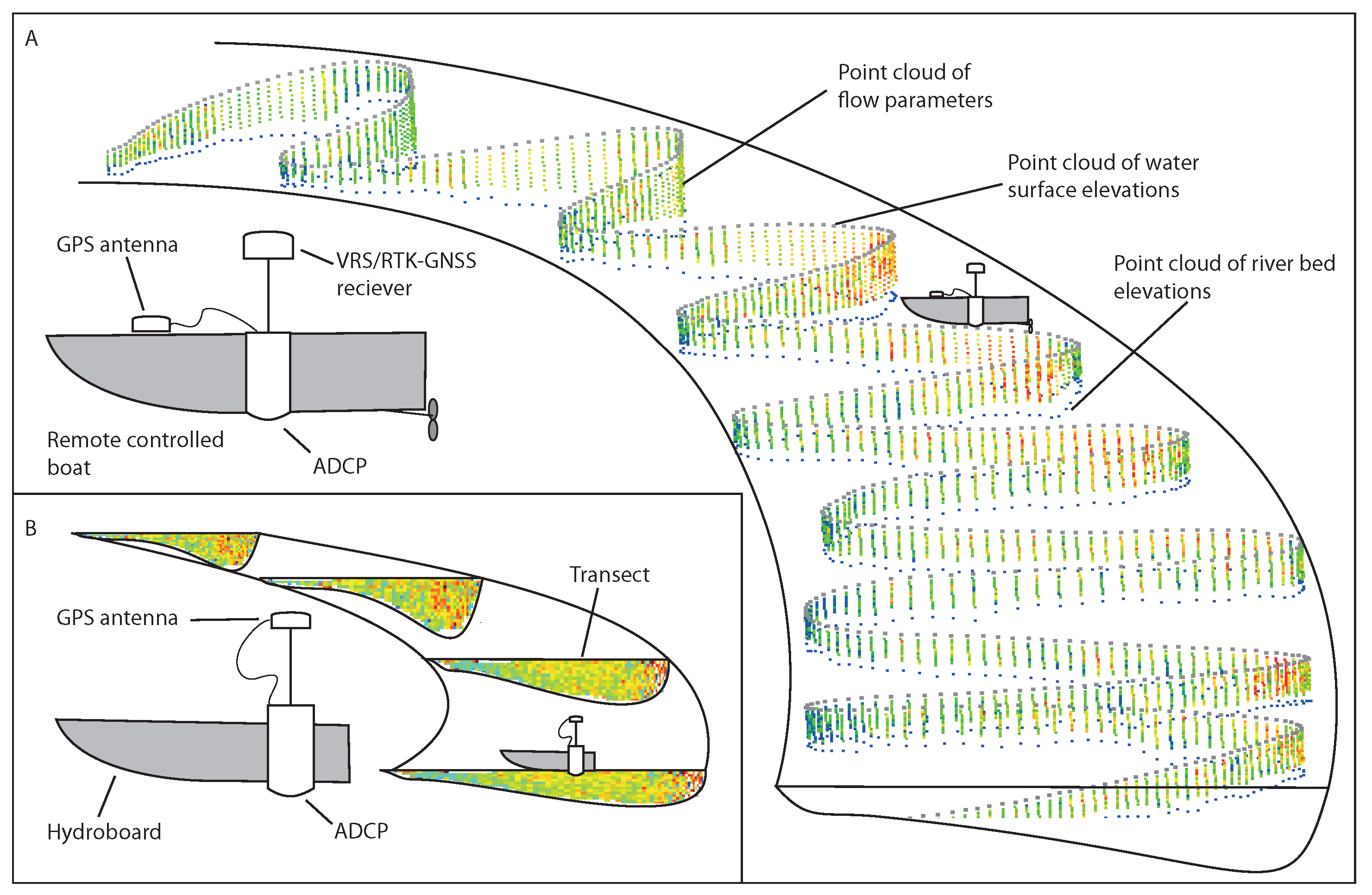
Figure 2.
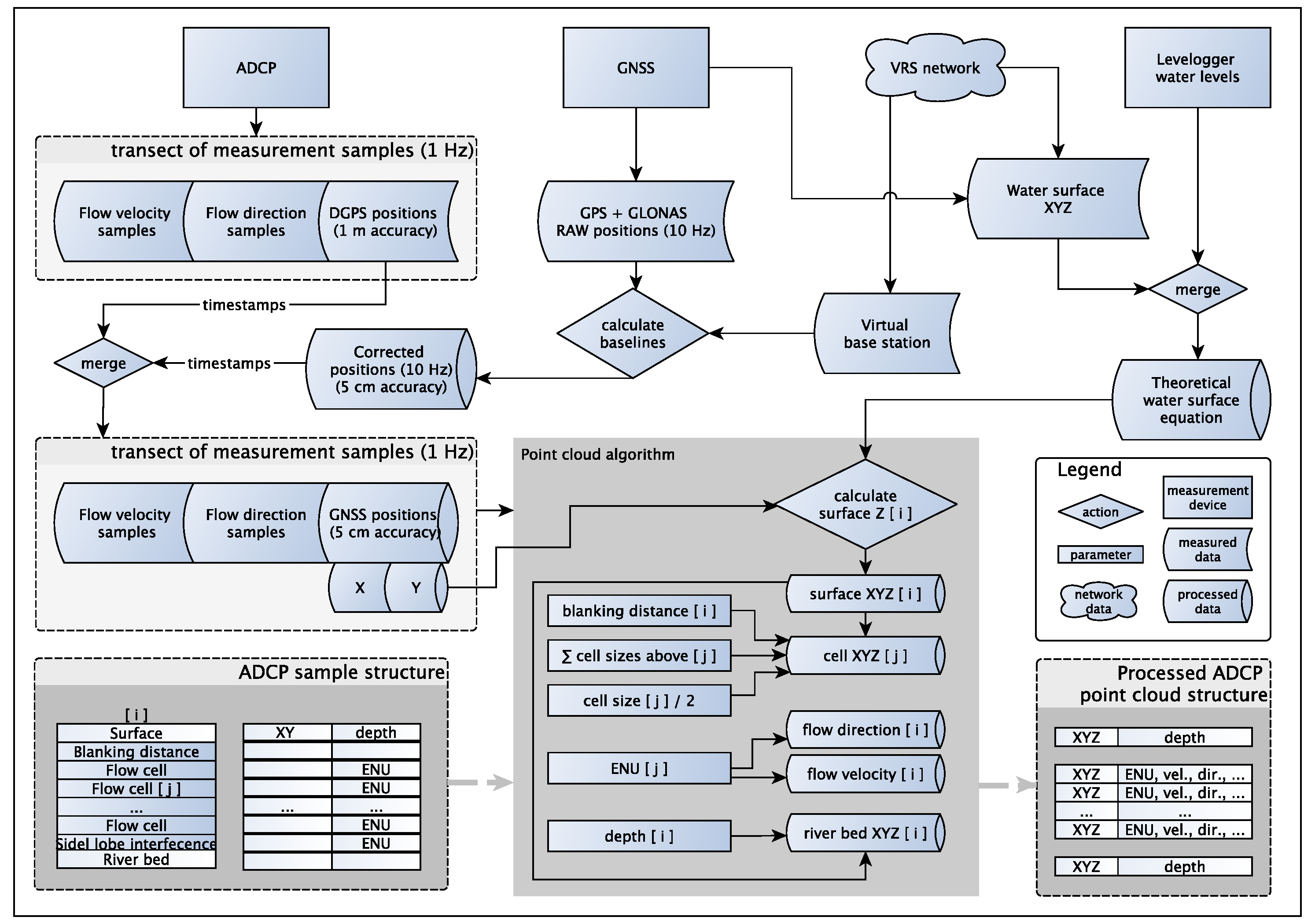
Diagram of the flow measurement set-up and concept. (A) The new spatial modeling of flow vectors as a 3D point cloud containing surface points, flow velocity and direction points in the water column and river bed elevation points; (B) This subfigure contrasts the more traditional method of representing flow as a series of transects.
3.1. Field Data
We conducted field measurements during a nine-day period (16–24 May 2013) that included the rising stage of the spring flood. Flow measurements were conducted daily at the meander bend AOI and every second day over the whole reach studied. Measurements of the meander bend AOI took about two hours to complete.
3.1.1. Remote-Controlled ADCP
We used a Sontek RiverSurveyor M9 ADCP mounted to a custom-built remote-controlled mini-boat (RCflow) to survey a dense pattern of flow measurements at the meander bend AOI. The boat is 1.43-m long and 0.425-m wide with the sensor emerging from the hull without its edge protruding at a water depth of 0.06 m. The hull is designed to minimize drag and turbulence, so that the boat can move against a fairly strong current and cause minimal interference to the measurements. RCflow makes it possible to survey even shallow reaches in sub-meter depths that cannot be accessed by larger boats. The boat is propelled by an electric motor powered by either NiCad or LiPo battery sets providing 20,000 mA/h. This allows for uninterrupted measurements exceeding 2 h, depending on flow conditions and the load required.
To measure the long reaches of the study area, we mounted a Sontek S5 ADCP to a Hydroboard floating platform attached with a pole to a motorboat (
Figure 3). This allowed us to cover a greater distance and better cope with the current than the battery-operated RC boat. We aimed for boat speeds not exceeding 1 ms
−1.
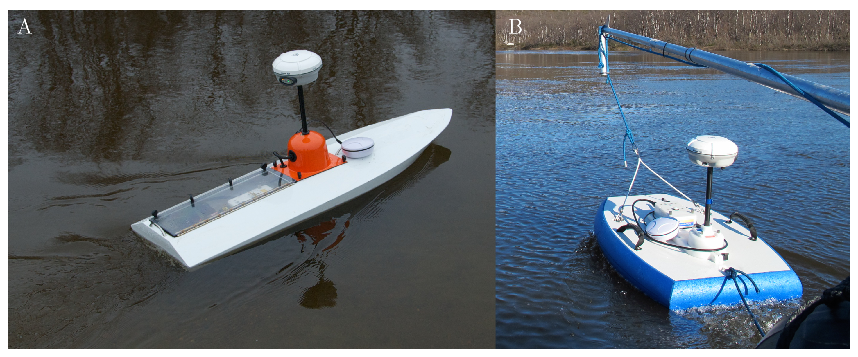
Figure 3.
ADCP-GNSS set-up on a remote-controlled boat (A) and on the Hydroboard tethered to a zodiac (B). A Trimble R8 GNSS receiver is mounted on the GPS pole of the ADCP exactly above the sensor, and the ADCP’s GPS antenna is mounted on the deck of the vessel.
Figure 3.
ADCP-GNSS set-up on a remote-controlled boat (A) and on the Hydroboard tethered to a zodiac (B). A Trimble R8 GNSS receiver is mounted on the GPS pole of the ADCP exactly above the sensor, and the ADCP’s GPS antenna is mounted on the deck of the vessel.
Both ADCPs had the SmartPulseHD feature enabled. Using this measurement mode, the sensor simultaneously emits coherent and incoherent pulses, potentially at multiple frequencies, and a processing algorithm selects the best return signal for the given water depth and velocity. The Sontek M9 uses 3.0-MHz, 1.0-MHz and 0.5-MHz and the S5 uses 3.0-MHz and 1.0-MHz pulses. The ADCP sample measurements were carried out in discharge measurement mode using the ADCPs’ differential GPS (DGPS) for tracking. Bottom tracking was not an option, because the sandy river bed is mobile during the spring flood. Measurements were collected in a zig-zag pattern as very long transects and later exported as raw data in MATLAB format. The ADCPs measure one sample (also referred to as an ensemble) each second, and each sample is divided vertically into separate cells, also referred to as bins. The number of cells depends on water depth, and the cell height is dynamically adjusted depending on depth and speed. Measurement cells may be as small as 2 cm in shallow (<1.5 m), slow moving (<0.4 ms−1) water or as large as 2 m in depths over 20 m. In our case, depths did not exceed 4 m, so the maximum cell size was 0.2 m.
By design, ADCPs average the flow of increasingly large areas into one measurement cell, with increasing distance from the sensor. That is, the measurement sample is in the shape of a pyramid consisting of different layers [
9,
29]. Each layer in the sample pyramid is one measurement cell. The true horizontal size of the measurement cell depends on the angle of the receivers on the sensor. Both Sontek ADCPs have the receivers arranged in a Janus configuration at a 25° angle. This means that, typically, the first cell measured after the blanking distance [
30] (the space too close to the sensor to measure, generally 25 cm) is 0.03 m
2; at a 1-m depth, the cell is 0.45 m
2, and at 2 m depth, the cell is 1.77 m
2 in area, while both cells may be the same thickness, say 0.1 m. Conceptually, however, the measurement sample is treated as a column of stacked cells, each of the same size, the width of which depends on the distance between consecutive samples, which depends on the boat speed. The measured value is often considered as a point located at the center of the cell, vertically and horizontally [
9] centered under the instrument. In fact, the center position of the cell that the measured value is assigned to is never actually measured, since the sensor integrates measured return signals from the four beams that surround the center point, but do not actually cover the area directly below the sensor.
3.1.2. Positioning (GNSS)
Creating 3D point clouds of flow data requires accurate absolute positioning of each measurement. In order to obtain the best possible absolute positioning, we mounted a Trimble R8 Global Navigation Satellite System (GNSS) operating in virtual reference station (VRS) mode onto the RiverSurveyor’s GPS antenna pole instead of the ADCP’s own GPS antenna, which, even when using real-time kinematic (RTK) correction, only achieves a relative positional accuracy of 2 cm, due to the fact that the base station estimates its own position using its own GPS antenna, and does so anew, every time the base station is booted. This gives the ADCP’s positional data DGPS-level accuracy in absolute terms, even though the points within one measurement have RTK-level precision relative to each other. If it were possible to set up the ADCP’s RTK base station over a known reference point and input those coordinates to the station along with the necessary offsets at millimeter accuracy, the use of a second GNSS would not be necessary. The location of the base station’s antenna cannot be input using Sontek’s RiverSurveyor Live software, making an external GNSS solution necessary. However, in the interest of completeness, it should be noted that the more recent optional HydroSurveyor software does give the option to input base station coordinates, which results in absolute RTK-GPS positioning.
VRS-GNSS (also known as network RTK) is a virtualized version of RTK-GNSS, using real-time kinematic positioning, but rather than using a physical base station in the field, the VRS receiver gets its correction data through a GPRS-based (general packet radio service) Internet connection. A computing centre gathers real-time satellite data from a network of base stations around the country, based on which a virtual base station in the vicinity of the rover is computed and the virtual correction data transmitted to the receiver in real time. It is also possible to download the correction data at a later time for post-processing purposes. Given that the field site is within range of a GPRS network, the VRS system is much more convenient and faster to set up than a physical base station. Furthermore, the fact that the virtual base station can be located very closely to the measurement and can even be updated when measurements spread over a large area, minimizes baseline length-dependent errors common in GNSS positioning.
The Trimble R8 GNSS makes use of both the GPS and GLONASS satellite systems, which greatly improves coverage, particularly at these high latitudes. Despite having a large number of satellites available, a river channel remains a challenging environment for rapid and accurate GNSS positioning, particularly near steep banks. Fortunately, trees at the riverbank did not represent much of an obstacle during the spring flood, since they had not grown any foliage yet.
The Sontek’s own GPS antenna was mounted on the bow of the RCflow or the Hydroboard to collect satellite timestamp data (
cf. Figure 2 and
Figure 3). We use GPS timestamps later to merge the GNSS and ADCP data. The appropriate GPS offsets were included in the ADCP set-up parameters, so as not to affect the tracking ability of the ADCP. The integrated GPS receives differential corrections (DGPS) from the Satellite-based Augmentation System (SBAS) satellite network, giving it a nominal accuracy of 1 m or better. These DGPS data are used by the ADCP for tracking (
cf. Section 3.1.1).
The R8 GNSS was set to collect raw data at 10 Hz, while the RiverSurveyor’s internal GPS collects data at 1 Hz, concurrent with its flow measurements. Given that these measurements do not necessarily take place at the peak of each second and that, like many instruments, the specified 1-Hz interval of the ADCP is theoretical and exhibits slight variation about that value in reality, this made it necessary to collect the actual positioning data at 10 Hz. At that rate, it is impossible for the GNSS to process differential corrections in real time, so we opted to post-process the data and calculate the baselines using correction data from the VRS network. This process gives us positional data at a precision of ±0.05 m or better in XYZ. Measurements with lower estimated precision were discarded in post-processing.
The 10-Hz VRS-GNSS positional data were subsequently merged with the 1-Hz flow measurements using the GPS timestamps included in the data from the RiverSurveyor’s own GPS. The precision of the timestamp is 0.1 s, so the possible horizontal error introduced by this process is at most 0.5 × boat speed, that is, half the distance between two subsequent flow measurements, which, given boat speeds of <1 ms
−1, amounts to at most ±0.05 m.
Table 1 gives an overview of the number of GNSS points, ADCP points for each measurement day at the meander bend AOI, as well as the number of points remaining after merging the two datasets.
3.1.3. Water Level Data
Water levels were continuously measured along the study reach at 15-min intervals using pressure transducers (Solinst Gold Leveloggers) mounted to concrete slabs that were sunk to the riverbed at the beginning of the field work period and left to collect data throughout the ice-free period (
Figure 4). The pressure transducers of these devices have an accuracy of ±0.005 m. Seven Leveloggers were positioned throughout the study area, three of which were located at the meander bend under investigation, one upstream, one in the middle of the bend in the deepest part of the meander and one downstream of the bend (
Figure 5). The loggers were positioned far enough from the bank to be in deep enough water to remain submerged during summer low flow conditions.
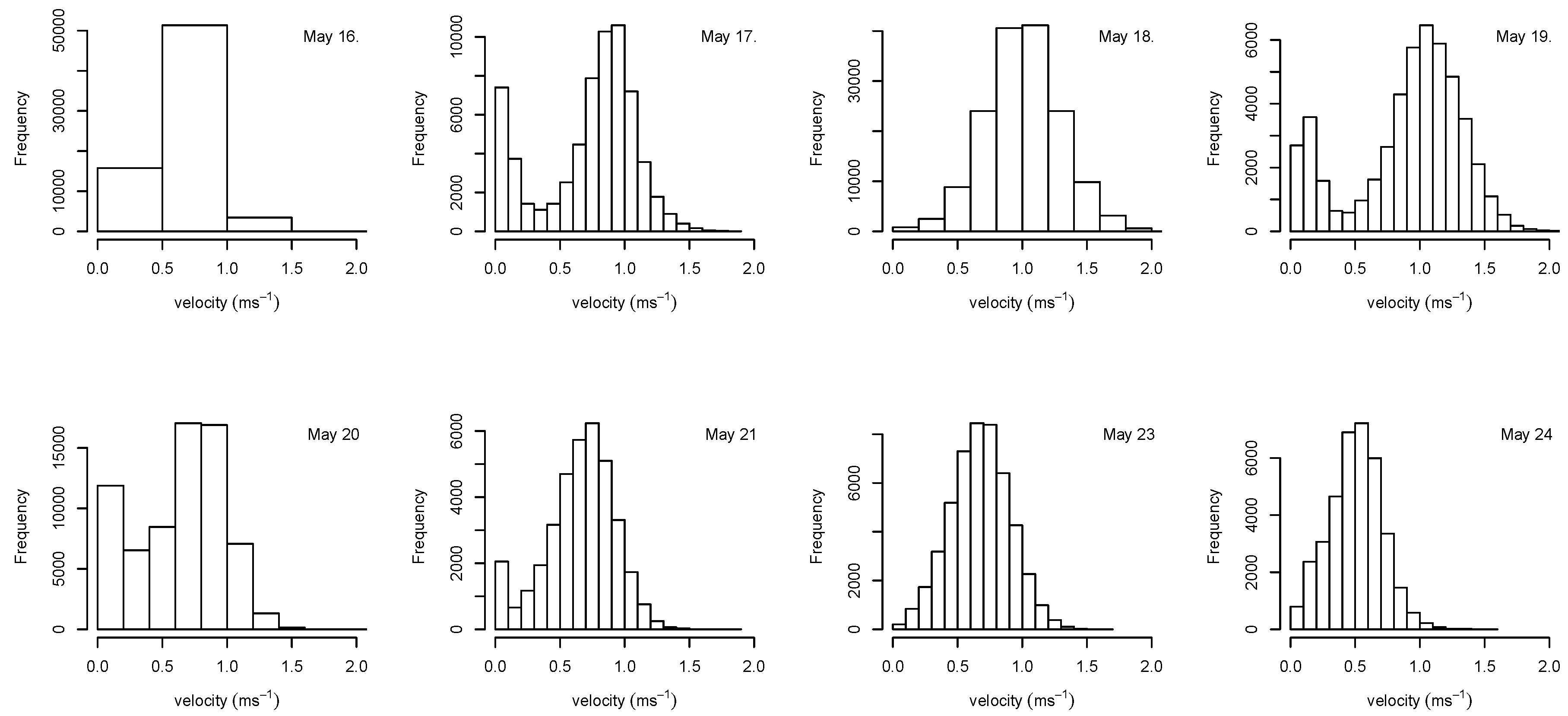
Table 1.
The number of points measured for each day at the meander bend AOI. GNSS points is the number of accepted points after baseline calculation (RMSE <0.05 m). ADCP points are raw measured point samples (ensembles). 3D points are the number of points in the point cloud for each day, and interpolated points are the number of points in the regular matrix interpolated from the original point cloud. 3D point density denotes the number of points per m3 in the meander bend AOI.
| Date | GNSS Points | ADCP Sample Points | 3D Points | Interpolated 3D Points | 3D Point Density in Meander (pts m−3) |
|---|
| May 6 | 82,823 | 7,444 | 70,556 | 2,587 | 15.2 |
| May 17 | 92,047 | 8,006 | 64,944 | 3,030 | 11.9 |
| May 18 | 497,716 | 17,293 | 155,584 | 3,243 | 2.2 |
| May 19 | 110,001 | 6,217 | 49,112 | 4,928 | 5.5 |
| May 20 | 96,532 | 8,552 | 69,397 | 4,983 | 7.7 |
| May 21 | 59,871 | 4,422 | 36,884 | 4,456 | 4.6 |
| May 23 | 87,028 | 6,368 | 49,744 | 5,703 | 4.8 |
| May 24 | 51,064 | 4,138 | 36,708 | 4,836 | 4.2 |
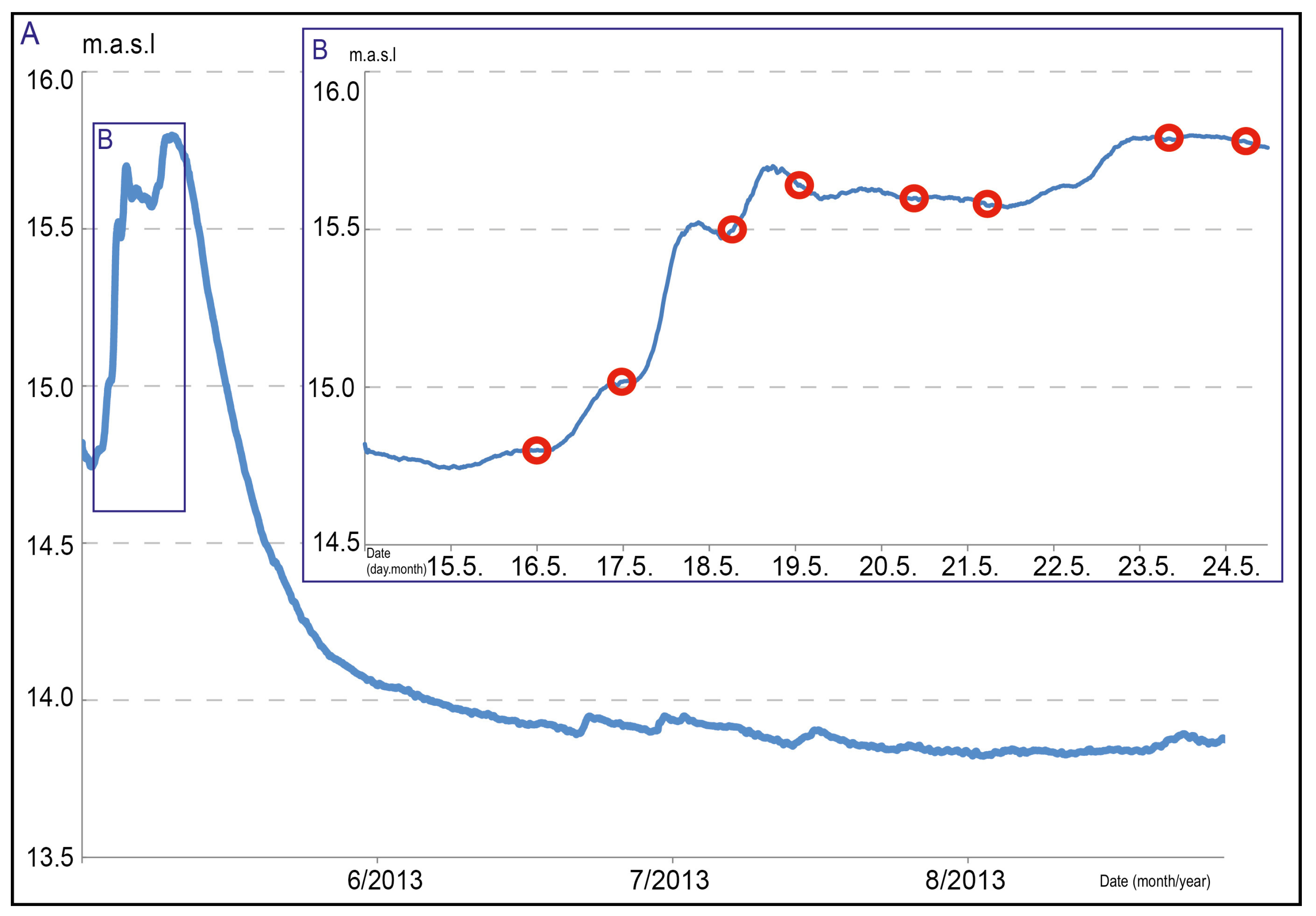
Figure 4.
(A) Hydrograph of the ice-free period for 2013 of the Pulmanki River; (B) The rising stage of the spring flood is in meters above sea level (m.a.s.l). ADCP-flow measurement times are indicated with red circles.
Figure 4.
(A) Hydrograph of the ice-free period for 2013 of the Pulmanki River; (B) The rising stage of the spring flood is in meters above sea level (m.a.s.l). ADCP-flow measurement times are indicated with red circles.
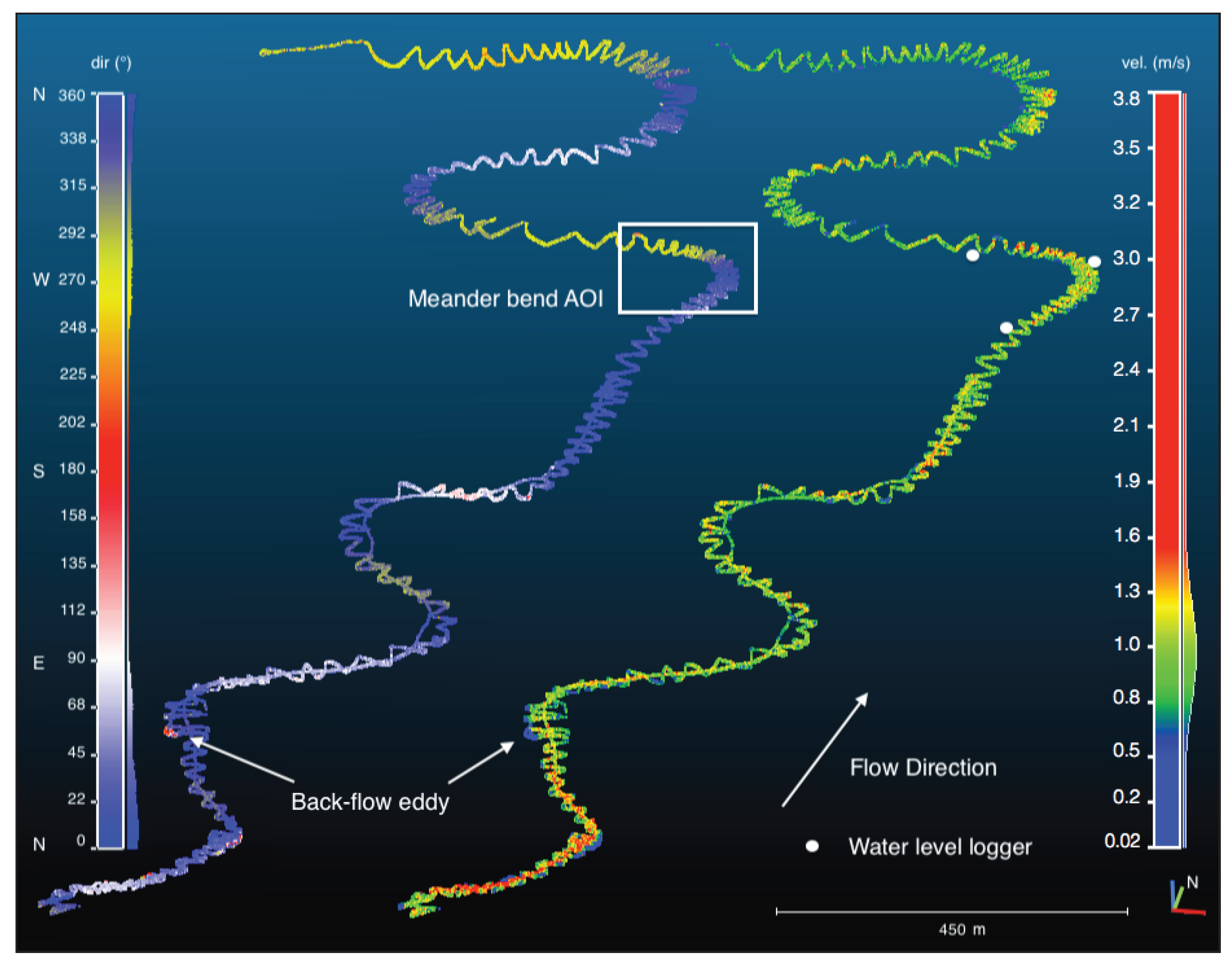
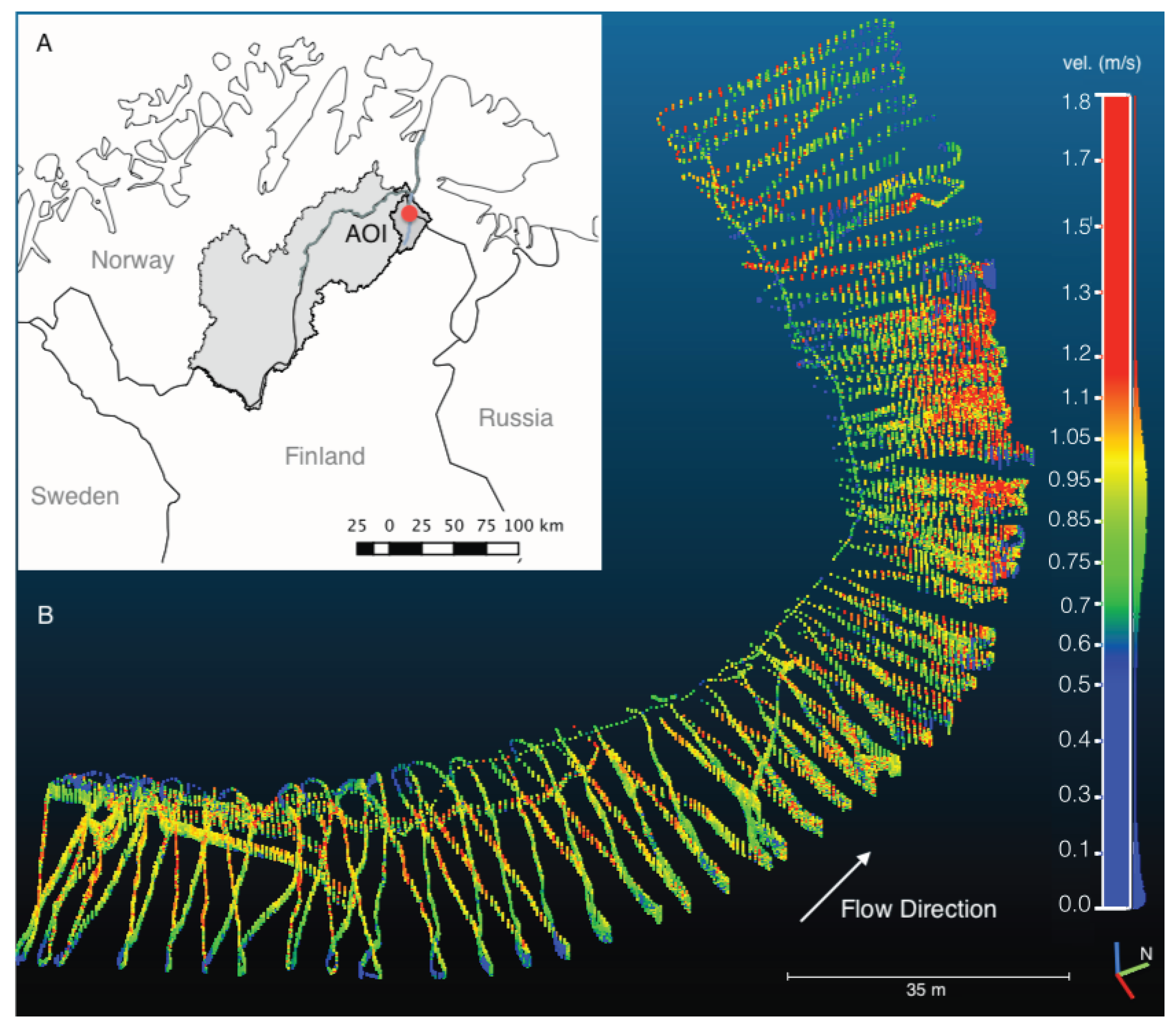
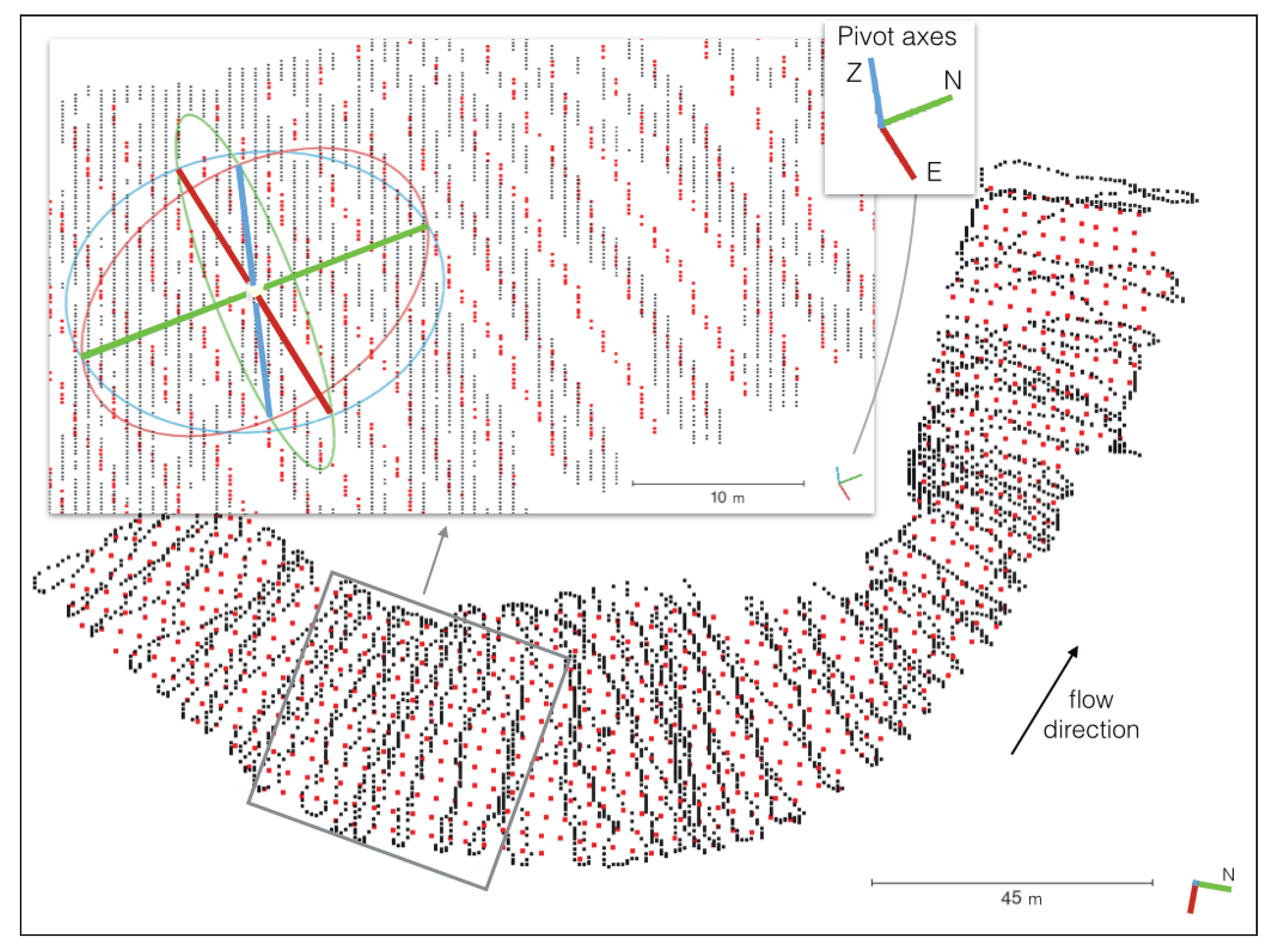
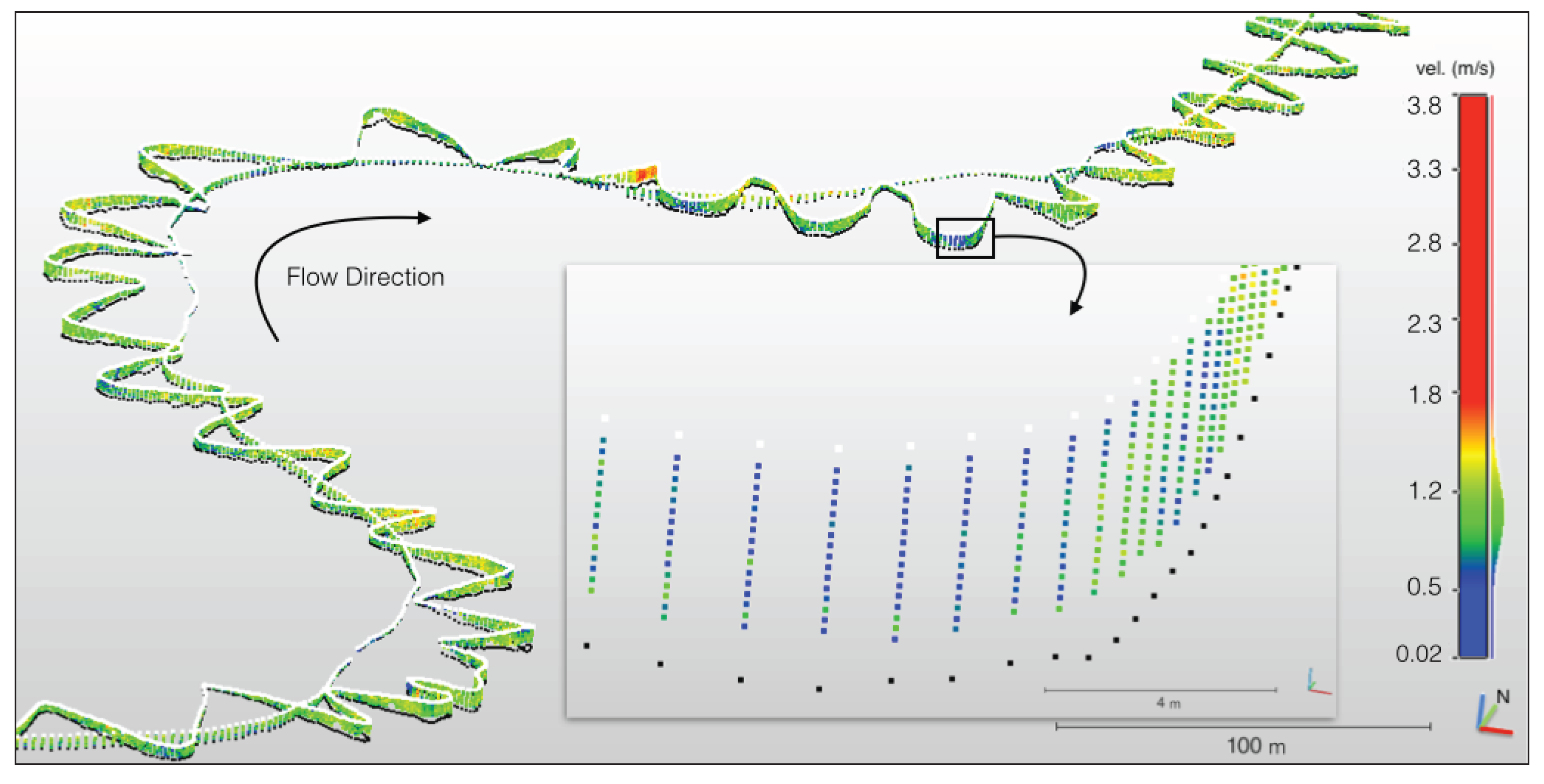
Figure 5.
Point cloud of raw measured flow data of the whole study reach (3.7 km) on 18 May 2013 looking downstream. The left-hand plot shows flow directions in degrees from the north and the right-hand plot shows flow velocities in m/s. A back-flow eddy location is clearly detectable in the plot of flow directions. The location of the meander bend AOI is indicated by a box, and the approximate locations of the water level loggers are indicated by three points. The actual water level loggers were located about 2 m from the shore at low water, but for ease of visualization, approximate locations are shown here.
The water levels were measured at the beginning and the end of the study period using VRS-GNSS topography point measurements. The topography point method involves measuring a series of consecutive points and averaging the resulting coordinates in order to increase accuracy by averaging small positional errors that may result from slight movements of the GNSS receiver. This results in a measurement with better than 2-cm precision [
31], which is suitable, given that the gradient of the river reach translates to a height difference of 0.2 m from the upstream to the downstream end of the reach. RTK-GNSS has previously been successfully used for water surface reconstructions [
32,
33,
34].
The Leveloggers log pressure and temperature data. A Barologger was located near the middle of the study reach to collect atmospheric pressure data for post-processing the pressure data of the Leveloggers into water depths.
Figure 4 shows the hydrograph measured by the water level loggers at the meander bend AOI for the ice-free period of 2013.
3.2. Data Processing
All ADCP data were exported to MATLAB format. The GNSS data were post-processed using VRS correction data from the Finnish virtual reference station network (
http://www.vrsnet.fi). Baselines were calculated, and points with a positional accuracy better than 0.05 m were retained and exported as CSV (
Table 1), including UTC timestamp information.
Further processing was carried out in R [
35].
Figure 6 outlines the conceptual processing flow. The GNSS position data were merged with the ADCP flow data using the GPS timestamps. The continuous water level measurements were used to create a localized time-specific water surface model. The water surface model is created by fitting a plane through the water surface elevations at the three level logger locations at the time of measurement:
where a, b and c are the level logger points; x, y and z are their respective coordinates and d is the distance from a level plane. Given the locations of the water level loggers (
Figure 5) with the upstream and downstream logger near the inside of the meander bend and the middle logger near the outside of the bend at the bend apex, we consider that this surface accounts for the possible superelevation of the water surface that is expected to be found in meander bends. In reality, though, at this particular meander bend, this effect is smaller than the vertical accuracy of the GNSS.
Figure 6.
Conceptual process of creating a point cloud of flow data from ADCP, virtual reference station (VRS)-GNSS and water level measurements. A simplified conceptual view of the original ADCP sample structure is shown, where one measurement sample [ i ] consists of a series of superimposed flow measurement cells [ j ], each of which contains flow parameters. This is contrasted with the processed point cloud structure, where each cell becomes its own unit with spatial information i.e., a 3D spatial point, as well as additionally computed flow parameters (direction from north, velocity), calculated from the ENUvalues of the original cells, that is the velocity magnitude to the east, the north and up. Here, the individual point elements are shown superimposed in the “processed ADCP point cloud structure”, only to show how their positions relate to the original measurement structure.
The flow data were registered to this water surface in order to avoid small remaining inaccuracies in the vertical component of the positioning. Whereas an accuracy of 5 cm or better horizontally is more than adequate for the purpose of 3D flow measurements in a river, in the vertical, this can leave a notable roughness to the water surface that was not present in the field. This artificial surface roughness would propagate to all measurement points in the water column. The water surface of the Pulmanki River is very calm, even during high water, with at most small ripples caused by wind (
cf. Figure 3). For measuring purposes, the water surface can be considered flat. We therefore consider the Levelogger-based water surface to be more accurate as vertical positioning than each measurement’s individual GNSS-measured elevation. The variation in the water surface elevations during the measurement period was considerably smaller than the vertical precision of the VRS-GNSS (
Table 2). The water surface elevation of each flow measurement sample was thus added to the dataset.
The ADCP automatically compensates tilting of the sensor caused by movement of the boat using its internal inertial measurement unit (IMU). The tilt sensor of the ADCP has a angular resolution of 1°.
The RiverSurveyor ADCP measures one sample each second. A sample is one vertical measurement (ensemble) that is divided into a number of cells (bins). In effect, this splits each vertical into a number of measurements, each with its own flow direction and velocity. The number of cells per sample depends on water depth and is dynamically adjusted by the RiverSurveyor’s internal algorithms. In practice, the cell size varies between 0.02 and 0.2 m.
The raw flow velocity measurements for each cell for each beam for each sample were used to calculate 3D flow vectors for each measurement cell. Flow directions were calculated in degrees clockwise from north, and horizontal velocity was calculated using ENU velocity components. This allows representing velocity as a magnitude parameter independent of flow direction.
In order to create a 3D point cloud of 3D flow data, the elevation of each measurement cell was calculated:
where
Ce is the elevation of a flow measurement cell;
Ws is the Levelogger-based water surface elevation at the sample-specific location;
C1 is the depth of the first measurement cell, that is the blanking distance (this varies for each sample, but is generally around 0.25 m);
n is the number of cells in a given sample and
Cs is the cell size of a given sample. This locates the sample elevation vertically in the center of the cell in question, in line with the conceptual location of ADCP measurements (
cf. Section 3.1.1). Similarly, river bed elevation was calculated by subtracting measured depth from the water surface elevation.
Thus, a point cloud of flow measurements was created, containing XYZ coordinates for each measurement, ENU coordinates of measured flow velocities, as well as flow velocity, direction, water surface, water depth, bed elevation and a UTC timestamp.
These points were subsequently interpolated in 3D using MATLAB to create a regular 3D matrix of points to create an evenly-spaced point cloud that is somewhat easier to visually analyze than the raw measured data. The point cloud was interpolated at different densities: 1 m, 2 m, 3 m and 4 m horizontally and 0.2 m vertically. The best interpolation density among these was determined to be 3 m horizontally and 0.2 m vertically. This is closest to the actual spacing of the measured data when considering the spacing of the zig-zag pattern, and while creating a large number of points, it is computationally manageable and visually not overwhelming, so that interpretation of the flow patterns is actually possible. The vertical spacing was selected to correspond to the most common large cell size of the ADCP measurements. A 0.2-m vertical spacing also results in a fair number of layers in shallow water without being overwhelming in deeper sections.
Figure 7 illustrates the spatial relation of the interpolated point cloud data to the originally measured point cloud data.
Table 2.
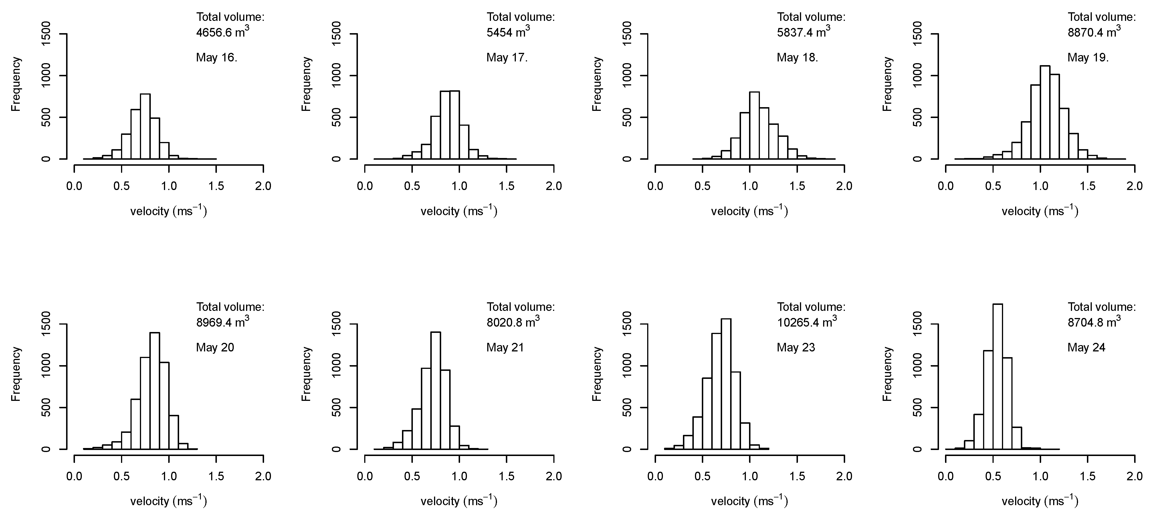
Results of the 3D-interpolated point clouds for Venesärkkä for each day: time of measurement, temperature (°C) mean T and standard deviation σ T during measurement period, water level elevation mean wl (metres above sea level) and standard deviation σ wl, slope (m), minimum velocity min v, mean velocity v, maximum velocity max. v (ms−1), min, mean and max. depths d (m), discharge Q (m3s−1), total volume of water vol (m3), volume of water moving at velocities of <0.5 m3, 0.5–1.0 m3, 1.0–1.2 m3 and >1.2 m3.
Table 2.
Results of the 3D-interpolated point clouds for Venesärkkä for each day: time of measurement, temperature (°C) mean T and standard deviation σ T during measurement period, water level elevation mean wl (metres above sea level) and standard deviation σ wl, slope (m), minimum velocity min v, mean velocity v, maximum velocity max. v (ms−1), min, mean and max. depths d (m), discharge Q (m3s−1), total volume of water vol (m3), volume of water moving at velocities of <0.5 m3, 0.5–1.0 m3, 1.0–1.2 m3 and >1.2 m3.
| Day | Time | T | σ T | wl | σ wl | Slope | Min d | d | Max d | Min v | v | Max v | Q | vol | vol < 0.5 | vol 0.5–1 | vol 1–1.2 | vol > 1.2 |
|---|
| 16 | 19:30–21:35 | 5.0 | 0.056 | 14.818 | 0.006 | 0.0010 | 0.35 | 1.38 | 2.61 | 0.12 | 0.72 | 1.43 | | 4656.6 | 306.0 | 4249.8 | 88.2 | 12.6 |
| 17 | 17:00–19:00 | 6.2 | 0.084 | 15.025 | 0.007 | 0.0013 | 0.30 | 1.55 | 2.83 | 0.17 | 0.88 | 1.52 | 35.28 | 5454.0 | 90.0 | 4329.0 | 937.8 | 97.2 |
| 18 | 19:20–19:40 | 5.0 | 0.002 | 15.493 | 0.002 | 0.0008 | 0.59 | 1.99 | 3.40 | 0.46 | 1.10 | 1.84 | 57.81 | 5837.4 | 3.6 | 1711.8 | 2552.4 | 1569.6 |
| 19 | 13:41–15:25 | 3.5 | 0.100 | 15.64 | 0.004 | 0.0006 | 0.37 | 2.12 | 3.62 | 0.17 | 1.06 | 1.82 | 66.00 | 8870.4 | 70.2 | 3013.2 | 3835.8 | 1951.2 |
| 20 | 17:57–20:05 | 4.7 | 0.163 | 15.601 | 0.001 | 0.0001 | 0.33 | 2.09 | 3.67 | 0.12 | 0.82 | 1.29 | 47.63 | 8969.4 | 300.6 | 7810.2 | 851.4 | 7.2 |
| 21 | 12:52–14:06 | 3.8 | 0.035 | 15.597 | 0.001 | 0.0000 | 0.38 | 2.12 | 3.63 | 0.20 | 0.72 | 1.24 | 42.16 | 8020.8 | 586.8 | 7342.2 | 90.0 | 1.8 |
| 23 | 19:59–21:37 | 9.3 | 0.040 | 15.787 | 0.001 | 0.0000 | 0.39 | 2.25 | 3.90 | 0.10 | 0.69 | 1.19 | 46.42 | 10265.4 | 1087.2 | 9068.4 | 109.8 | 0.0 |
| 24 | 21:17–22:25 | 10.1 | 0.019 | 15.763 | 0.000 | 0.0000 | 0.28 | 2.17 | 3.84 | 0.09 | 0.54 | 1.12 | 33.33 | 8704.8 | 3076.2 | 5626.8 | 1.8 | 0.0 |
Figure 7.
Comparison of original (black) vs. interpolated (red) data example of 19 May in plane view. The insert shows a close-up viewed at an angle (a 3D pivot sphere is included for spatial reference), to illustrate how the vertical dimension compares between the measured and interpolated point clouds. The point density in the interpolation matrix is sparser vertically and compared to the original sample line, along the line. The density is similar when considering the line spacing of the original zig-zag pattern. The pivot axes in this 3D plot, as well as in all subsequent plots indicate the view angle, with the green north-south axis pointing towards the north (substituting the north arrow), the red east-west axis pointing towards the east and the blue vertical axis pointing upwards, normal to the N-E plane.
In order to create a realistic interpolation of the 3D flow structure in the stream, a Delaunay triangulation-based interpolation was applied to interpolate the velocity, angle, direction, surface elevation and depth values of the raw point cloud. A 3D network of triangular planes is created using the scattered raw points; the network is then sampled into a regular voxel space (a 3D matrix) of a defined resolution (here, 3 m × 3 m × 0.2 m). A natural neighbor interpolation is used to interpolate values of each voxel (each cell in the matrix) using the Delaunay network. All input data, as well as all the interpolations use the exact same section of the river. That is, all point clouds have the same length of thalweg; only the width of the water area changes with the stage of the flood.


 ,
, 


