Seasonal Demand Dynamics of Residential Water End-Uses

Abstract

Water demand prediction by end-use at an appropriate spatial and temporal resolution is essential for planning water supply systems that will supply water from a diversified set of sources on a fit-for-purpose basis. Understanding seasonal, daily and sub-daily water demand including peak demand by end-uses is an essential planning requirement to implement a fit-for-purpose water supply strategy. Studies in the literature assume that all indoor water uses except evaporative cooler water use are weather independent and do not exhibit seasonal variability. This paper presents an analysis undertaken to examine seasonal variability of residential water end-uses. The analysis was repeated using two sets of data to ensure the validity of findings. The study shows that shower water use is significantly different between winter and summer, in addition to irrigation, evaporative cooler and pool water end-uses, while other water end-uses are not. Weather is shown to be a significant determinant of shower water use; in particular it affects shower duration which increases with lower temperature. Further analysis on shower water use suggests that it is driven by behavioural factors in addition to weather, thus providing useful insights to improve detailed end-use water demand predictions.

1. Introduction

Supplying water to the world’s population between now and 2030 from an absolutely finite supply is identified as a clear and significant challenge [1]. This is due to the fact that only one percent of the world’s total water is fresh and drinkable and is poorly managed [1]. While population growth is a key factor affecting water scarcity, improving living standards, urbanisation and supply variability due to climate change also add pressure on water scarcity in different parts of the world [2,3,4,5].

Australia is a highly urbanised country (89 per cent of the population lives in towns and cities), and the urban population is expected to grow rapidly over the next 40 years [6]. Furthermore, Australia has experienced prolonged and severe drought conditions from 2002 to 2008 particularly, in the south eastern part of the country [7,8]. This is believed to be as a result of climate change [8]. Dependence primarily on the water stored in dams makes Australian water supply heavily vulnerable to drought [6]. All these factors together with a growing population have increased pressure on Australian cities to act on water availability and secure it for the future. This pressure has intensified demand management programs such as education, permanent water saving rules, rebates, incentives, water restrictions, provision of rain water tanks and other methods of alternative water supplies. In this context, the need for detailed knowledge of water end-use behaviours has led water authorities and researchers to conduct studies to understand water use patterns of households including detailed surveys and end-use measurement programs. A large number of water end-use studies around the world in the last decade [5,9,10,11,12,13] highlight the importance of the detailed knowledge that these end-use studies are generating, irrespective of their high costs. This also emphasises the need for a fine scale understanding of water end-uses in addressing the critical issue of water scarcity. In Australia, a number of studies have been conducted on water end-uses [14,15,16,17,18] to understand percentages of water use by each end-use, their variability over the years and over seasons, factors that affect water end-uses, and to measure end-use variables (e.g., frequency, duration, flow rate, peak demands and demand patterns).

Available water end-use data were used to build a number of end-use models across the world [2,9,19,20,21,22]. While the scope and output scales of these models are different, the majority of these models predict water end-uses at small temporal and spatial scales including daily or sub-daily scale and at per person or household scale [2,19,21,22,23]. Blokker et al. [21] showed the importance of end-use water demand predictions at small time scales (per second or per minute at household scale) for modelling of water quality of drinking water distribution systems. Rathnayaka et al. [24] showed the importance of end-use water demand predictions at small time and spatial scales for planning water supply sources employing the fit-for-purpose water use concept. For both these purposes, it is important to investigate temporal and spatial variability of water end-uses and their underlying variables. Though, the available end-use studies have widened the knowledge on the variability of demographic characteristics and appliance efficiency across households and their effect on water end-use, studies on temporal variability of water end-use are limited. Although the models that predict demand at sub-daily time scales consider diurnal demand patterns of all water end-uses [19,21], studies on seasonal and daily variability of end-uses are limited to outdoor uses [2,9,19,23]. This is because of the prevailing assumption that indoor water uses except evaporative cooler water use are non-seasonal and the short periods for which end-use data are available. This study is aimed to expand the scope of the previous studies mentioned above by testing the variability of all residential water end-uses between winter and summer. This has not been addressed in these previous studies. Consistent with this identified gap, this paper analyses the seasonal variability of residential water end-uses between winter and summer. The study discusses shower and irrigation water use in detail as end-uses that have seasonal variability. The importance of these end-uses lies in that they are the largest water end-uses (about 30% or more in total) in Australia according to the recent studies [17,22]. The study also identified temperature as a sensitive variable for those seasonal water end-uses. This understanding is crucial to improve the accuracy of forecasting seasonal peak water demand which in turn supports planning and management of urban water resources.

2. Data

2.1. Water End-Use Data and Survey Data

This analysis makes use of measured water end-use data and survey data of household characteristics. The household water end-use data were collected by Yarra Valley Water (YVW) and City West Water (CWW) in winter 2010 and summer 2012. These water utilities have used high resolution water measurement meters (known as smart meters) to measure household water use. The data were captured using data loggers at five-second intervals which was then disaggregated into individual end-use events using the Trace Wizard^© (Trace Wizard^© is developed by Aquacraft Inc. Water Engineering and Management [25]) water use analysis tool [17]. This data set includes details on shower, toilet, tap, bath, dishwasher, clothes washer, irrigation, evaporative cooler, pool and leaks end-uses. Tap use includes all kitchen, laundry and bathroom taps. The data on volume, duration and flow rate for each individual event at five-second intervals enabled the derivation of daily end-use event frequency, event duration and daily volume of end-uses at individual household level.

Demographic and household data were collected from the households at the time of installing household data loggers. These data include information on household size, typology of dwelling, and the presence of different water using appliances such as dishwasher and evaporative cooler. Both YVW and CWW data samples consisted of similar features in terms of household size, dwelling type and presence of children as shown in Table 1.

Table 1. Key characteristics of data samples. YVW: Yarra Valley Water; CWW: City West Water.

Key Characteristics	YVW	CWW
Average household size	3.1	3.1
Dwelling composition	Flat-3%, Semi-detached-11%, Detached-86%	Semi-detached-5%, Detached-95%
Households with children under 12 years	With children-29%, Without children-71%	With children-33%, Without children-67%

Table 1. Key characteristics of data samples. YVW: Yarra Valley Water; CWW: City West Water.

Key Characteristics	YVW	CWW
Average household size	3.1	3.1
Dwelling composition	Flat-3%, Semi-detached-11%, Detached-86%	Semi-detached-5%, Detached-95%
Households with children under 12 years	With children-29%, Without children-71%	With children-33%, Without children-67%

While Section 3.1 describes the steps taken to minimise data uncertainties, we recognize that there are other sources of uncertainty. They arise from measurement device errors, and assuming household size over the observation period during which there may have been temporal variation in the number of occupants in households. These sources of uncertainty are not quantified in this study.

2.2. Data Collection

Water authorities in Melbourne installed high-resolution water meters and data loggers in 337 households [17]. Our study used data from 117 households collected by YVW and CWW in this measurement program. YVW is the biggest water retailer in Melbourne and provides service to over 1.7 million people in Melbourne’s northern and eastern suburbs [26]. CWW provides service to approximately 276,000 residential customers in Melbourne’s central business district, inner and western suburbs [27]. Winter data were collected during a two week period in July and August, 2010 by both utilities. In Melbourne, winter months are from June to August and summer months are from December to February. As the summer of 2010/2011 was unusually wet (average summer rainfall was 102 mm/month compared to 51 mm/month of long-term average rainfall) and hence does not represent regular summer in Melbourne [17], the authorities collected summer data in a two week period in January 2012.

2.3. The Situational Context

The end-use data was collected while Stage 1 and Stage 3 water restrictions were in place. Stage 1 water restrictions allowed garden and lawn watering using a hand held hose fitted with a trigger nozzle at any time while other irrigation systems were subject to day and time limitations [28]. Filling pools up to 2000 litres and washing vehicles were allowed under Stage 1 water restrictions with minor limitations on the method [28]. Stage 3 water restrictions banned lawn watering using drinking water completely while garden watering was allowed but limited to specified time of the day and only using either a hand held hose fitted with a trigger nozzle or dripper systems [28]. Filling swimming pools, spas and water toys were restricted and washing vehicle at home was subject to severe limitations under Stage 3 water restrictions [28]. The winter of 2010 was under Stage 3 water restrictions while the summer 2012 was under Stage 1 water restrictions [29]. However, both these restrictions did not impose limitations on indoor water end-uses. Irrigation water use was not seriously restricted during summer but had restrictions on the method of water application. Water restrictions may have affected pool water use but filling of pools up to 2000 L was allowed under Stage 1 water restrictions which were in place during the summer measurements.

Table 2 shows the weather conditions during the 13 days in which data from two locations-YVW area and CWW area were collected for this study. Weather data were obtained for the weather stations nearest to the study areas. These are station number 086071 (Melbourne Regional Office) for YVW and 086039 (Flemington Racecourse) and 087031 (Laverton) for CWW [30]. It is important to note that this study did not use all the collected end-use data during this period, while weather data were observed only for days that end-use data were used in this study. Section 3.1 still provide further details on data collection.

Table 2. Weather data in YVW and CWW area during summer and winter data collection period. YVW: Yarra Valley Water; CWW: City West Water.

Weather Variables	YVW Summer	CWW Summer	YVW Winter	CWW Winter
Average maximum daily temperature (°C)	27.8	29.4	13.6	14.9
Average minimum daily temperature (°C)	18.5	15.9	8.0	6.2
Number of days exceeded 30 °C	7	7	-	-
Long-term average maximum daily temperature of the month/s which data were collected (°C)	25.9	25.7	15	14.9
Average rainfall (mm/d)	0.6	0.2	2.0	2.1
Number of days with no rainfall	10	10	3	6
Long-term average rainfall of the month/s which data were collected (mm/d)	1.6	1.4	1.6	1.5

Table 2. Weather data in YVW and CWW area during summer and winter data collection period. YVW: Yarra Valley Water; CWW: City West Water.

Weather Variables	YVW Summer	CWW Summer	YVW Winter	CWW Winter
Average maximum daily temperature (°C)	27.8	29.4	13.6	14.9
Average minimum daily temperature (°C)	18.5	15.9	8.0	6.2
Number of days exceeded 30 °C	7	7	-	-
Long-term average maximum daily temperature of the month/s which data were collected (°C)	25.9	25.7	15	14.9
Average rainfall (mm/d)	0.6	0.2	2.0	2.1
Number of days with no rainfall	10	10	3	6
Long-term average rainfall of the month/s which data were collected (mm/d)	1.6	1.4	1.6	1.5

The CWW area shows overall a warmer and drier weather compared to YVW area during the study period (Table 2) although the magnitude of the difference is not considerable. While, the maximum daily temperature of the period is closely representative of its long-term (all year) averages in winter, summer temperatures were slightly higher than the long-term averages (Table 2). Further, daily average rainfall recorded during the measurements was lower in summer than the long-term averages while rainfall recorded during winter measurements was slightly higher than the long-term averages (Table 2). Therefore, the effect of rainfall on seasonal variability of water end-uses was not studied in this study.

3. Method

The data were analysed using a number of statistical techniques explained in Section 3.2 to observe the seasonal variability of water end-uses. The analysis was repeated using two sets of data collected by YVW and CWW to ensure the validity of findings. This section discusses the data preparation and the statistical techniques used in this study.

3.1. Data Preparation

Although the expected sample size of the end-use data collected by CWW and YVW was 100 households in each sample, a smaller number of households were willing to participate in the survey during the summer program. Winter and summer data from the same group of households was used in the analysis to ensure consistency of data and to eliminate variations between samples due to people’s behaviour and household characteristics. This has further reduced the sample size to 61 households in the CWW sample and 56 households in the YVW sample, but improved the accuracy of results.

The summer data collection period consists of a greater number of days in which people are not at home during the whole day and hence, the total water use recorded in those days is limited to leakage losses. Only days in which there was an actual use of water, were selected for the analysis to avoid the effect of people being absent from home. Days in which people were present at home, were identified as those days in which non-leakage end-uses have occurred. The number of days fitting these criteria was greater in winter. In addition, the days that data was collected in the measurement program did not overlap among all households. To test the response of all households to the same weather conditions, we used data from the same set of days from all participating households in winter and in summer. This reduced the number of days for which data was analysed to 13 in each season for each household in each sample (26 days in total for winter and summer). These steps allowed consistent comparison and interpretation of the difference in water use between winter and summer.

The average daily water end-use volume per person (L/p/d) (Litres per person per day) was estimated separately for winter and summer and for the YVW and CWW samples. This average was obtained from the per person water use of 56 and 61 households in each sample. Although shower, toilet, clothes washer and tap uses were available in all households, bath and dishwasher were available from fewer households in each sample. A garden was present in all the houses except two houses in the YVW sample. Therefore, the calculation of average daily end-use volume (L/p/d) in households with bath, dishwasher and irrigation only includes those households where those end-uses are present.

3.2. Data Analysis

The end-uses analysed in this study include shower, toilet, tap, bath, irrigation, dishwasher and clothes washer, for which records are available in both seasons. However, evaporative cooler and pool water use data were only available during summer. As such, they are considered to be seasonal end-uses.

Scatter plots, descriptive statistics and paired t-tests were used to observe the seasonal difference in water end-uses [31]. Paired t-tests allowed accounting for variability in water use of same set of households between the two seasons resulting in a smaller error term, thus increasing the sensitivity of the hypothesis test or confidence interval. The condition of normality of the data for the test was verified tested showing that the data met the condition. Probability plots of all end-use data showed that data are normally distributed and showed p values greater than 0.1 at 95% confidence interval.

Shower and irrigation water end-uses were further analysed using the Ordinary Least Squares (OLS) regression method [32]. The data used in this analysis show that they are in agreement with the assumptions of OLS regression analysis in that the regression model has linear coefficients, residuals have a mean of zero, all predictors are uncorrelated with the residuals, residuals do not show serial correlation, residuals have a constant variance, no multicolinearity and residuals are normally distributed [33].

4. Seasonal Dynamics of Water End-Uses

4.1. Seasonal Variability of Water End-Uses in the YVW Data Sample

Shower, toilet and irrigation water end-uses in the YVW data sample are considerably different between winter and summer while end-uses, tap, bath, dishwasher and clothes washer do not show such difference (Figure 1). While shower and toilet water use were lower during summer compared to winter, irrigation use was as expected higher during summer (Figure 1). Irrigation water use was recorded even in winter and showed a similar magnitude to dishwasher and bath water end-uses. Further, daily irrigation water use in summer shows a clear increase with increasing maximum daily temperature (Figure 1). This behaviour was not observed in other end-uses.

Figure 1. Scatter plots of seasonal water end-use volume and maximum daily temperature categorised by season for YVW data.

Figure 1. Scatter plots of seasonal water end-use volume and maximum daily temperature categorised by season for YVW data.

Table 3 shows that the p value for shower, toilet and irrigation water use is lower than a commonly chosen α value (0.05) that suggests a statistically significant difference in those water end-uses between summer and winter (Table 3). The p values for other water end-uses are greater than 0.05 and their confidence interval includes zero (Table 3), thus providing evidence that there is no statistically significant difference in those water end-uses between the two seasons.

Table 3. Summary of outcomes from the paired t-tests using YVW data (L/p/d).

End-use	Average water use		Mean difference (Summer-Winter)	95% CI for difference	T value	p value
	(L/p/d)
	Summer	Winter
Shower	31.03	39.01	−7.98	(−10.07, −5.89)	−8.33	0.00
Bath	3.31	4.71	−1.4	(−3.45, 0.64)	−1.49	0.16
Toilet	18.41	21.12	−2.71	(−3.89, −1.54)	−5.04	0.00
Tap	20.82	20.15	0.67	(−0.97, 2.31)	0.89	0.39
Dishwasher	1.78	1.97	−1.9	(−0.48, 0.10)	−1.42	0.18
Clothes washer	19.67	22.37	−2.7	(−8.51, 3.11)	−1.01	0.33
Irrigation	20.13	3.72	16.41	(9.70, 23.12)	5.33	0.00

Table 3. Summary of outcomes from the paired t-tests using YVW data (L/p/d).

End-use	Average water use		Mean difference (Summer-Winter)	95% CI for difference	T value	p value
	(L/p/d)
	Summer	Winter
Shower	31.03	39.01	−7.98	(−10.07, −5.89)	−8.33	0.00
Bath	3.31	4.71	−1.4	(−3.45, 0.64)	−1.49	0.16
Toilet	18.41	21.12	−2.71	(−3.89, −1.54)	−5.04	0.00
Tap	20.82	20.15	0.67	(−0.97, 2.31)	0.89	0.39
Dishwasher	1.78	1.97	−1.9	(−0.48, 0.10)	−1.42	0.18
Clothes washer	19.67	22.37	−2.7	(−8.51, 3.11)	−1.01	0.33
Irrigation	20.13	3.72	16.41	(9.70, 23.12)	5.33	0.00

As expected, irrigation water use shows the greatest mean difference between the two seasons compared to others (51.3 L/hh/d or 16.4 L/p/d). Shower water use is also significantly different between summer and winter and the difference on average is 25.0 L/hh/d or 8.0 L/p/d. Although toilet water use in summer and winter is statistically different, the magnitude of the difference is rather small (8.5 L/hh/d or 2.7 L/p/d) and equal to half of an average flush volume that is 5.6 L/event [17].

4.2. Seasonal Variability of Water End-Use in CWW Data Sample

The seasonal difference in shower and irrigation water use between summer and winter for CWW corroborates the results of the same analysis carried out using CWW data (Figure 2 and Table 4).

Figure 2. Scatter plots of water end-use volumes and maximum daily temperature categorised by season for CWW data.

Figure 2. Scatter plots of water end-use volumes and maximum daily temperature categorised by season for CWW data.

Table 4. Summary of outcomes from the paired t-tests using CWW data (L/p/d).

End-Use	Average Water Use		Mean Difference (Summer-Winter)	95% CI for Difference	T value	p value
	(L/p/d)
	Summer	Winter
Shower	44.49	39.59	4.90	(1.20, 8.59)	2.88	0.01
Bath	5.26	6.94	–1.68	(–5.95, 2.60)	–0.85	0.41
Toilet	20.18	20.53	–0.35	(–1.828, 1.109)	–0.53	0.60
Tap	29.61	19.01	10.60	(8.531, 12.674)	11.15	0.00
Dishwasher	2.12	1.99	0.13	(–0.459, 0.703)	0.46	0.66
Clothes washer	18.79	24.39	–5.60	(–9.57, –1.63)	–3.08	0.01
Irrigation	34.08	4.47	29.61	(16.71, 42.51)	5.00	0.00

Table 4. Summary of outcomes from the paired t-tests using CWW data (L/p/d).

End-Use	Average Water Use		Mean Difference (Summer-Winter)	95% CI for Difference	T value	p value
	(L/p/d)
	Summer	Winter
Shower	44.49	39.59	4.90	(1.20, 8.59)	2.88	0.01
Bath	5.26	6.94	–1.68	(–5.95, 2.60)	–0.85	0.41
Toilet	20.18	20.53	–0.35	(–1.828, 1.109)	–0.53	0.60
Tap	29.61	19.01	10.60	(8.531, 12.674)	11.15	0.00
Dishwasher	2.12	1.99	0.13	(–0.459, 0.703)	0.46	0.66
Clothes washer	18.79	24.39	–5.60	(–9.57, –1.63)	–3.08	0.01
Irrigation	34.08	4.47	29.61	(16.71, 42.51)	5.00	0.00

Results from CWW data analysis show that shower, tap and irrigation water use are significantly greater during summer compared to winter (Figure 2 and Table 4). The average irrigation water use is 29.6 L/p/d (92.7 L/hh/d) greater in summer than in the winter. This difference in irrigation water use between summer and winter in the CWW data is considerably greater than the seasonal difference in YWV data of 16.4 L/p/d. This difference could be attributed to the difference in weather in the two locations as discussed in Section 2.3 that is the CWW area is located in an area of lower precipitation and comparatively higher temperatures than the YVW area. Furthermore, summer irrigation water use shows an increase in water use with increasing maximum daily temperature, a trend that was also observed in shower and tap uses (Figure 2). This increase in shower use with maximum daily temperature in summer may be explained by an increase in shower frequency, which is discussed in Section 5. However, it is difficult to explain the seasonal difference in tap water use based on the available data. It is possible that some irrigation use may have been classified as tap use because people do bucket watering to irrigate their vegetable gardens and it could not be identified separately in the absence of water use diaries. In addition, clothes washer water use in CWW data is greater in winter than summer (Table 4) but such difference was not observed in YVW data. This difference could be due to one data point that shows the largest clothes washer water use in winter (Figure 2) that belongs to weekend. These 13 days over which the data had been collected in winter consisted of four weekend days while the summer data collection period consisted of three weekend days which is approximately similar.

In summary, both YVW and CWW data show that irrigation and shower water use are significantly different between winter and summer. This difference prompted an investigation in more detail of how and why these end-uses vary seasonally.

5. Weather Sensitivity of Shower Water Use

Shower water use is the largest water end-use recorded in the 2010–2012 end-use measurement campaign and it is a common end-use for all households [34]. An important aspect of the data analysis is that shower water use is affected by weather. Beal and Stewart [16] explained the considerably lower shower water use recorded in South East Queensland (SEQ) in summer 2010–2011 (December 2010–February 2011) by the extremely wet weather conditions during this period in SEQ. This is additional evidence that weather affects shower water use. Table 5 compares winter and summer water use data from Melbourne with that in SEQ. Only the end-uses available in all households were compared to ensure the consistency of the comparison. SEQ data also agrees with our findings on seasonal water uses showing shower water use is seasonally different (Table 5).

Table 5. Comparison of average end-use water consumptions (L/p/d).

End-Use	Season	Average Water Use (L/p/d)-Melbourne		Average Water Use * (L/p/d) [16]
		YVW	CWW	SEQ
Shower	Summer	31.0	44.5	36.2
	Winter	39.0	39.6	42.7
Toilet	Summer	18.4	20.2	23.0
	Winter	21.1	20.5	23.7
Tap	Summer	20.8	29.6	27.4
	Winter	20.1	19.0	27.5
Clothes washer	Summer	19.7	18.8	26.5
	Winter	22.4	24.4	31.0

Note: *: Data were taken from winter 2010 and summer 2010/2011.

Table 5. Comparison of average end-use water consumptions (L/p/d).

End-Use	Season	Average Water Use (L/p/d)-Melbourne		Average Water Use * (L/p/d) [16]
		YVW	CWW	SEQ
Shower	Summer	31.0	44.5	36.2
	Winter	39.0	39.6	42.7
Toilet	Summer	18.4	20.2	23.0
	Winter	21.1	20.5	23.7
Tap	Summer	20.8	29.6	27.4
	Winter	20.1	19.0	27.5
Clothes washer	Summer	19.7	18.8	26.5
	Winter	22.4	24.4	31.0

Note: *: Data were taken from winter 2010 and summer 2010/2011.

While shower water use shows sensitivity to weather, the YVW data shows less shower water use in summer than in winter in contrast to CWW data. Thus a relationship between temperature and shower volume cannot be identified. In order to further elucidate this question, shower water use was further analysed from the frequency and duration of shower events which are key behavioural variables determining shower water use.

The average shower duration is higher in YWV data than in CWW data both in winter and summer (Table 6 and Figure 3). In addition, the average shower duration in winter is longer than in summer (Figure 3), possibly due to longer time needed for the water to reach a warm temperature, people keeping the tap open without interrupting and enjoying long warm showers in cold weather. This provides evidence of a possible relationship between average shower duration and weather.

Table 6. Average shower frequency and shower duration in two seasons in CWW and YVW data samples.

Variable	Data Source	Season	Mean	Standard Deviation
Average shower frequency/p/d	CWW	summer	1.07	0.12
		winter	0.82	0.04
	YVW	summer	0.68	0.05
		winter	0.73	0.04
Shower duration (Seconds/event)	CWW	summer	365	20.17
		winter	400	17.98
	YVW	summer	373	14.74
		winter	460	22.15

Table 6. Average shower frequency and shower duration in two seasons in CWW and YVW data samples.

Variable	Data Source	Season	Mean	Standard Deviation
Average shower frequency/p/d	CWW	summer	1.07	0.12
		winter	0.82	0.04
	YVW	summer	0.68	0.05
		winter	0.73	0.04
Shower duration (Seconds/event)	CWW	summer	365	20.17
		winter	400	17.98
	YVW	summer	373	14.74
		winter	460	22.15

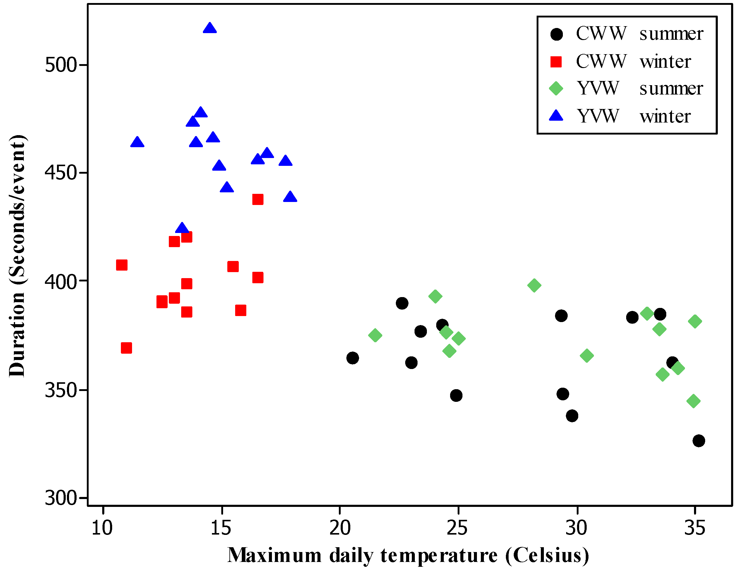
Figure 3. Scatter plot of average shower duration (seconds/event) and maximum daily temperature.

Figure 3. Scatter plot of average shower duration (seconds/event) and maximum daily temperature.

OLS Regression analysis between average shower duration (seconds/event) and maximum daily temperature (°C) shows a negative correlation between these two variables (Table 7). A p value lower than 0.05 suggests that the relationship is statistically significant (Table 7).

The ability to explain this difference in shower duration by temperature is moderate (R² = 0.43). This suggests that there are other causes involved in driving shower duration. Relative humidity which, is another weather variable that may have an effect on shower water use, of the two locations was found approximately similar (Relative humidity for YVW location for winter is 73%, for CWW location it is 79% and summer relative humidity for both locations is 63% [30]. Therefore, it may not have any impact. Since the respondents are from the same group of households, by ensuring consistency of other physical factors such as efficiency of showerheads and demographic factors such as age, the difference in shower duration can be ascribed to unobserved behavioural factors which need further study.

Table 7. Results of the regression analysis between average shower duration and maximum daily temperature.

Tested Variables	T value	p value	R2	Regression Coefficient
Average shower duration (Seconds/event) vs. maximum daily temperature (°C)	−6.11	0.000	0.43	–3.37

Table 7. Results of the regression analysis between average shower duration and maximum daily temperature.

Tested Variables	T value	p value	R2	Regression Coefficient
Average shower duration (Seconds/event) vs. maximum daily temperature (°C)	−6.11	0.000	0.43	–3.37

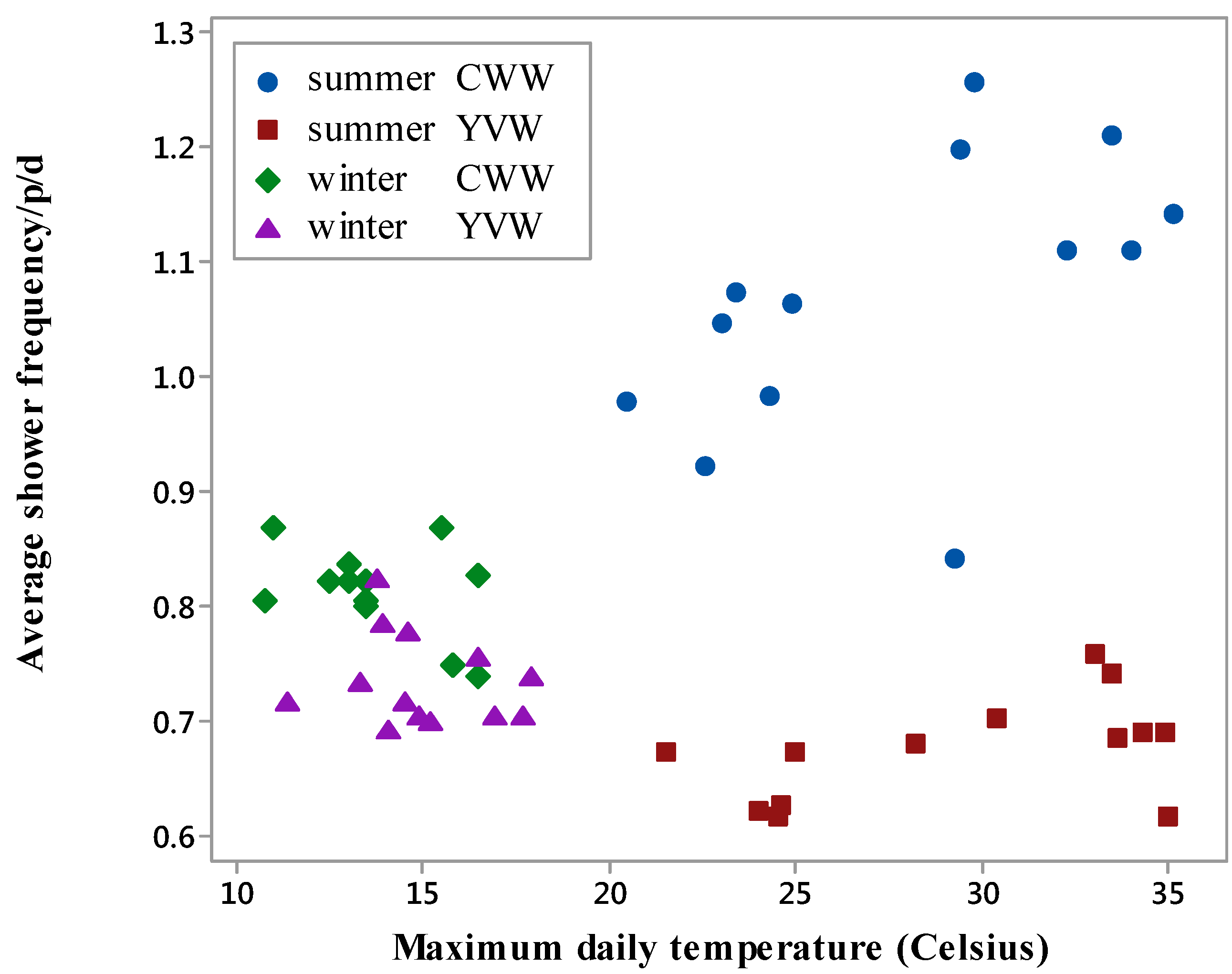
In addition to shower duration, shower frequency was also subjected to further analysis. The average shower frequency in CWW data is greater than in YVW data and the shower frequency in summer is higher than it is in winter (Table 6 and Figure 4), a fact that can be explained by comparatively warm and dry weather. Further, an increase in shower frequency is observed with increasing temperature in the CWW data sample (Figure 4). Conversely, the YVW data shows a slightly greater shower frequency in winter than in summer (Table 6). It must be noted that other outdoor activities such as swimming pools and spas during hot days can also affect in-house shower frequency in summer. A closer observation of the data confirms this assumption for the YVW data, showing considerable percentage of summer days (11%) with no shower use in YVW households while water use was recorded for all other end-uses.

Figure 4. Scatter plot of average shower frequency/p/d and maximum daily temperature.

Figure 4. Scatter plot of average shower frequency/p/d and maximum daily temperature.

In conclusion, considerably longer shower duration in winter in the YVW data may explain its greater winter shower water use, while greater shower frequency in summer in the CWW data may explain the greater summer shower water use. This leads to the conclusion that temperature affects shower water use and the likely but unverified impact on shower water use. These observations suggest that extreme weather conditions can increase shower water use as cooler weather increases shower duration while hot weather increases shower frequency, which is a noteworthy finding in terms of managing water demand with respect to extreme weather conditions projected for the future [35].

6. Weather Sensitivity of Irrigation Water Use

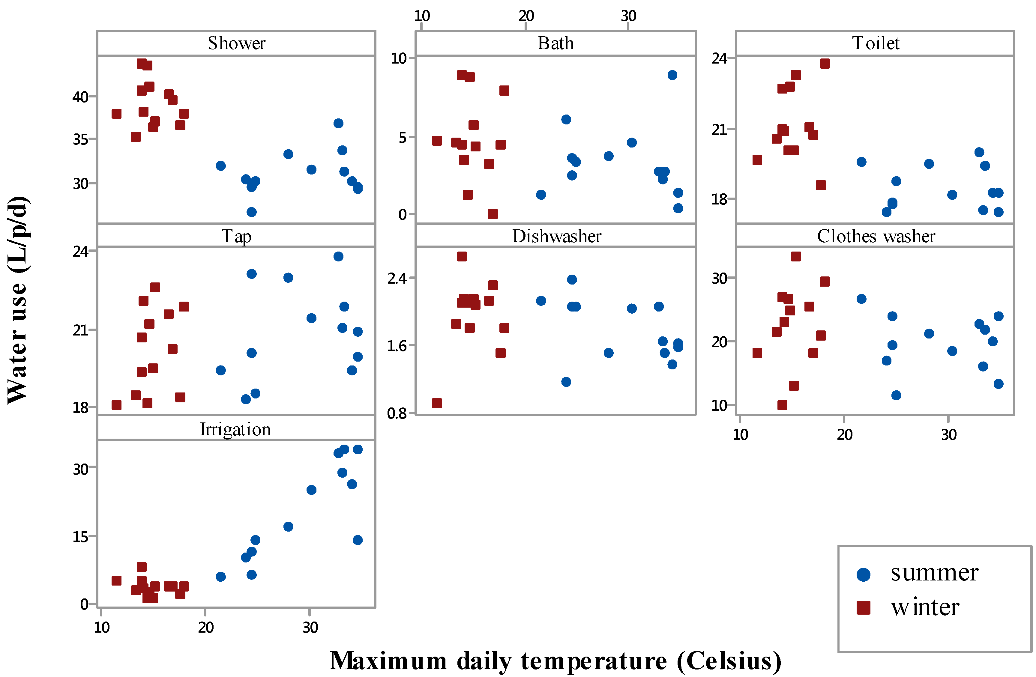
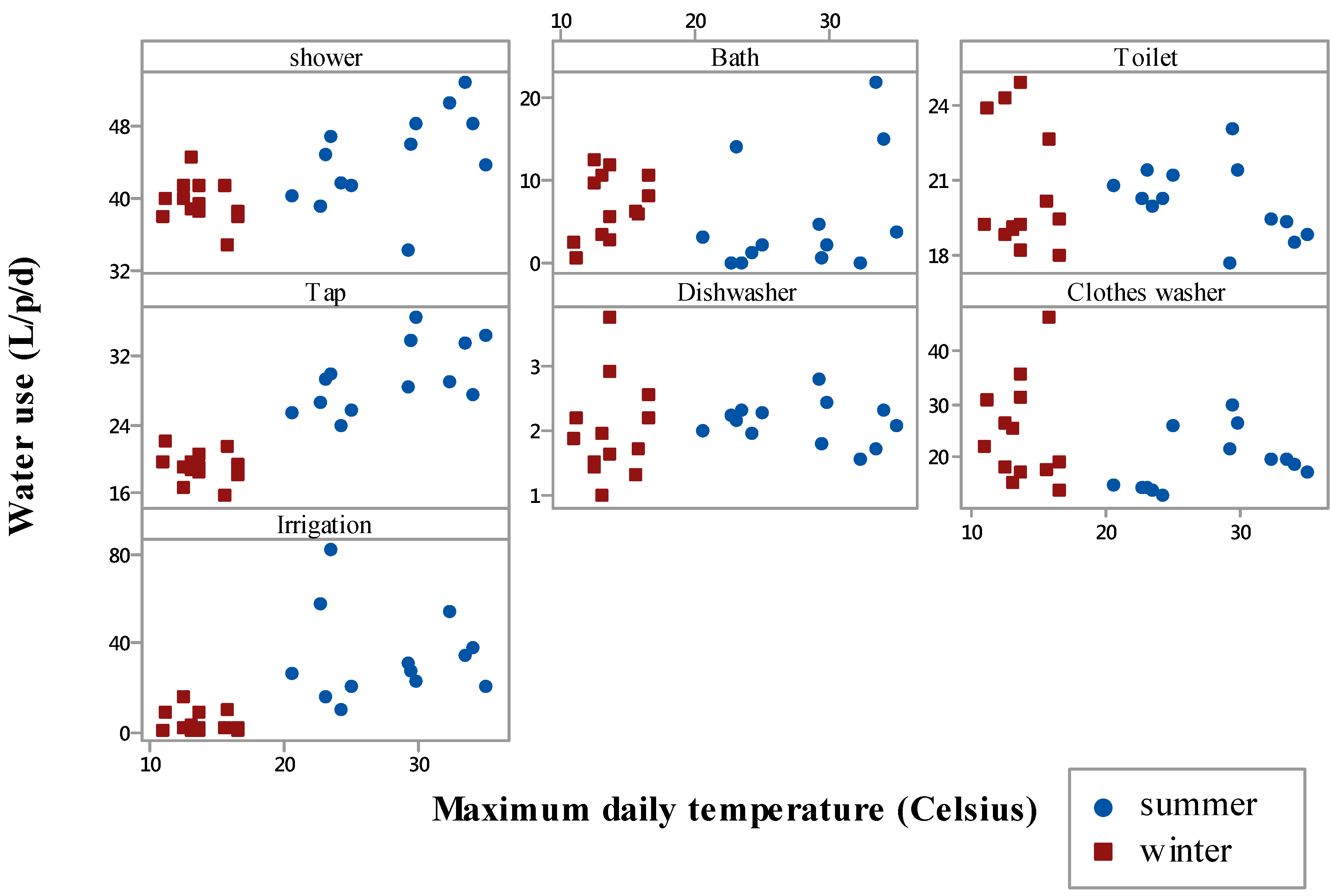
Irrigation is the second most predominant water use identified in the 2010–2012 end-use measurement campaign [34]. Both CWW and YVW data show that irrigation water use is greater in summer than in winter and increases with maximum daily temperature while winter irrigation does not show such a relationship (Figure 1 and Figure 2).

Further analysis between irrigation variables and maximum daily temperature was carried out using OLS regression analysis to investigate their relationship. This analysis was carried out using an ensemble of the CWW and YVW samples as they both show a relationship with temperature (Figure 1 and Figure 2).

The volume of irrigation water use shows a close relationship with maximum daily temperature (Table 8 and Figure 2) thus agreeing with the findings of Duncan and Mitchell [19] which show the maximum daily temperature is the best single explanatory variable of garden irrigation water use in Melbourne. The correlation of the occurrence of irrigation water use with maximum daily temperature is moderate and the correlations between average duration and flow rate with daily irrigation water use are poor (Table 8). These relationships were observed during average winter and summer conditions in Melbourne when people use efficient irrigation methods, predominantly responding to water restrictions in place. As such, a large number of other variables including garden size, behavioural factors, occurrence and magnitude of rainfall, irrigation method and availability of alternative water sources can affect irrigation water use. Further analysis would be needed to understand the effects of these explanatory variables. However, this is precluded by the lack of available data at present given that data is only available for a period of 13 days.

Table 8. Results of regression analysis between irrigation variables and maximum daily temperature.

Tested Variables	T value	p value	R2	Regression Coefficient	Coefficient of Variation
Average occurrence (times/hh/d vs. maximum daily temperature (°C)	7.14	0.000	0.58	0.01	50.97
Average duration (Seconds/d) vs. maximum daily temperature (°C)	2.64	0.012	0.15	77.53	85.97
Average event flow rate (L/min) vs. maximum daily temperature (°C)	2.39	0.022	0.13	0.10	20.05
Average volume (L/hh/d) vs. maximum daily temperature (°C)	8.38	0.000	0.65	4.55	102.43

Table 8. Results of regression analysis between irrigation variables and maximum daily temperature.

Tested Variables	T value	p value	R2	Regression Coefficient	Coefficient of Variation
Average occurrence (times/hh/d vs. maximum daily temperature (°C)	7.14	0.000	0.58	0.01	50.97
Average duration (Seconds/d) vs. maximum daily temperature (°C)	2.64	0.012	0.15	77.53	85.97
Average event flow rate (L/min) vs. maximum daily temperature (°C)	2.39	0.022	0.13	0.10	20.05
Average volume (L/hh/d) vs. maximum daily temperature (°C)	8.38	0.000	0.65	4.55	102.43

7. Conclusions

The purpose of this study was to understand the seasonal demand variability of water end-uses and to improve the current understanding of factors that influence the seasonal variability of residential water end-use. The study used two sets of data collected from CWW and YVW in Melbourne, Australia.

The study shows that bath, dishwasher, toilet, tap and clothes washer end-uses are not significantly different between winter and summer, while shower and irrigation, which are the main water end-uses are significantly different resulting in 6.5 and 23 L/p/d difference, respectively.

Weather is shown to be a significant determinant of shower water use; in particular as it affects shower duration which decreased with maximum daily temperature. Shower frequency shows an increase with maximum daily temperature in the CWW data set. However, the causes of this behaviour warrant further research since the absence of people from their residence during day time in the YVW data set may have affected the results. The results also suggest that shower water use may increase with extreme weather conditions as cooler weather increases shower duration while hot weather increases shower frequency. Irrigation water use exhibits seasonal difference in both the YVW and CWW data sets with greater summer consumption of 16.4 L/p/d and 29.6 L/p/d, respectively. This difference is partially explained (65%) by maximum daily temperature while study suggests many other variables, which need further research.

This analysis in turn can support modelling of residential end-use water demand, and inform the development of effective demand management programs such as awareness campaigns and supply-demand balance assessment of diversified water supply systems.