Hydraulic Conductivity Estimation Test Impact on Long-Term Acceptance Rate and Soil Absorption System Design

Abstract

The aim of this paper was to verify the common methods of hydraulic conductivity estimation for soil assessment in respect to wastewater disposal. The studies were conducted on three types of sandy soils. Hydraulic conductivity was determined using a scale effect-free laboratory method, empirical equations and compared with measurements estimated from a laboratory infiltration column with identified head loss. Based on the hydraulic conductivity values, the long-term acceptance rates (LTAR) [1] were calculated. The differences in LTAR values were about one order of magnitude smaller than differences in hydraulic coefficient. The study showed a good convergention of the results obtained from the constant head method (CHM) by solving the Glover Equation for medium and coarse sands. In low permeability soil (fine sand), the best result was obtained using CHM-a with a capillary rise consideration (a is a factor included in the flow in the unsaturated and saturated zones calculated from a capillary rise). From a practical point of view the relatively small value of LTAR underestimation (20%-for constant head method) is responsible for the extended surface area of the system and provides a security margin (the avoidance of clogging risk). The use of the falling head method, based on the Van Hoorn equation, can be said to be highly overestimated. For medium and coarse sandy soils the underestimation of LTAR calculated and based on CHM test determination is 14%–18%. The total cost of soil absorption system (SAS) designed-based on CHM in comparison to that designed-based on real hydraulic conductivity value in Poland is only about 7%–9% higher.

1. Introduction

Hydraulic conductivity is the main parameters used for estimation water and wastewater applicability in saturated soils.

Based on the determination of hydraulic conductivity the long-term acceptance rate can be calculated. The term “long term acceptance rate” (LTAR) is the daily volume of wastewater that can be applied over an indefinite period of time to a unit of soil surface area. LTAR values were determined using the equation [1]:

$$LTAR=5K_s-\frac{1.2}{{\log }_{10}{K}_s}$$

(1)

where,

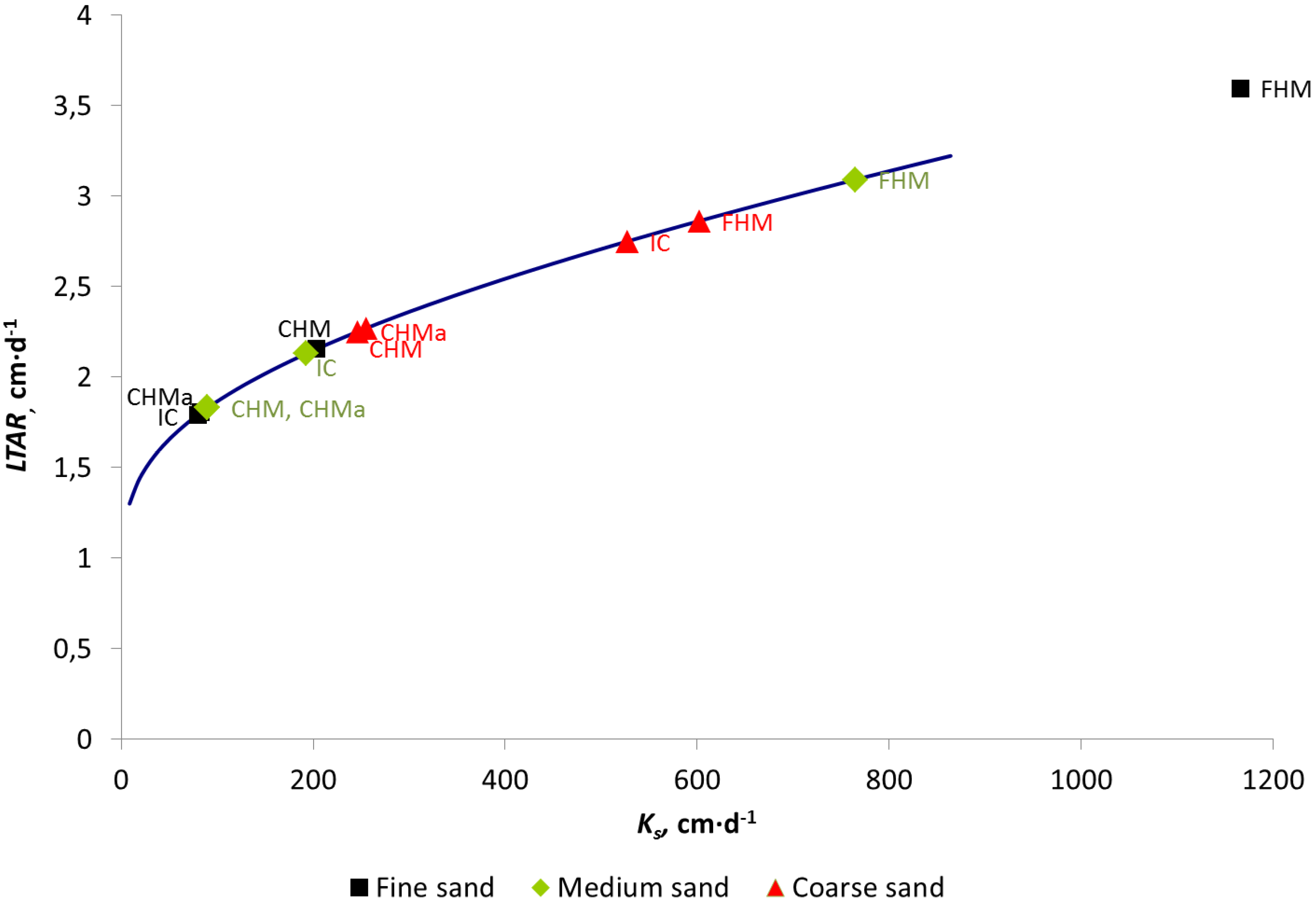
• LATR–long term acceptance rate, gal·ft⁻²·d⁻¹, the utilization range between 0.32 and 0.80 gal·ft⁻²·d⁻¹ (1.3 and 3.2 cm·d⁻¹);
• K_s–hydraulic conductivity, ft·min⁻¹.

Several studies can be found in the literature and related papers were published in accordance with LTAR [2,3,4].

There are many different methods to estimate hydraulic conductivity of soils under various conditions, which may have impact on hydraulic conductivity. For example, some methods are used to estimate hydraulic conductivity to obtain contamination migration velocity and others, to estimate hydraulic conductivity of soil for sub-surface disposal of waste-water. Some authors [5] have utilized the hydraulic conductivity decrease as a factor of biofilm growth (clogging factor).

Methods of estimation of hydraulic conductivity can be mainly divided into field and laboratory. The former are conducted in natural conditions where factors, such as temperature, pressure and the level of the water table, may affect the result. An additional advantage of field methods in comparison to laboratory ones is the opportunity to take into account the local conditions in a given research context. The most popular method among field methods is a percolation test which can be conducted in situ, where a given subsurface disposal system will be completed [6]. During the recent past, the percolation tests were modified and now can be divided into tests conducted in steady-state (constant head-CHM) and unsteady-state (falling head-FHM) conditions.

Laboratory methods can be divided into direct and indirect ones. Direct methods use soil samples with an unbroken or broken structure taken from where a subsurface drainage is planned. Hydraulic conductivity is often estimated using a filtration column where measurements are conducted in steady or unsteady conditions. This research is simple and inexpensive but the problem is how to obtain a representative size of soil sample. Indirect methods are based on information about the physical characteristics of investigated soils, e.g., bulk density, effective porosity, grain size distribution, and solid matrix properties, such as grain shape, pore shape, specific surface, tortuosity and organic matter content, to estimate hydraulic conductivity [7,8,9].

One of the first researchers who described the relationship between porosity and hydraulic conductivity was Slichter [10]. Aronovici [11] showed a correlation between the content of silts and clay in a cohesive soil and its impact on the soil hydraulic conductivity estimated in laboratory conditions. Oosterbaan and Nijland [12] reported that Smedema and Rycroft in 1983 presented the hydraulic conductivity in a range of soils as a function of grain size distribution. Additionally, the authors pointed out that in the case of soils with the same texture but different structure, the results of hydraulic conductivity can be differentiated a great deal more. De Ridder and Wit [13] described a method to estimate hydraulic conductivity using the ratio of irregular particles to regular ones contained in a sample measuring 1 cm in diameter. In the authors’ opinion, the range of method validity is limited only to homogeneous and isotropic soils, which are rather rare in nature.

Knowledge about grain size distribution can be used to calculate hydraulic conductivity using one of the well-known empirical formulae [14,15].

The empirical equations can be divided into two groups depending on the input data as follows:

• utilizing information about grain size distribution only, e.g., USBR (The United States Bureau of Reclamation) or Seelheim formula,
• demanding more information about the soil porosity or specific surface area, etc. as per the modified version of Hazen, the Krüger or Kozeny—Carman formula.

During the last few years the methods used to estimate hydraulic conductivity based on drainage porosity [16] have gained more popularity. In this paper the methods based on drainage porosity have not been verified by reason of difficulties in obtaining drainage porosity values.

There is no simple relation between wastewater infiltration rate and K_s decrease due to the complex nature of the clogging process and numerous related conditions and terms affecting such a process. There are many experimental research results showing that the infiltration rates through the biomat or sub-biomat soil layer in permeable, sandy soils can be between 1.4 and 7.5 cm/d [17,18,19]. The hydraulic gradient in fine sand below the biomat (clogging layer) was measured and its value came approximately to 7. For the minimum value of LTAR: 1.3 cm/d the corresponding K value is 8.64 cm/d and calculated (taking into consideration hydraulic gradient equal 7) permeability is about 61 cm/d. This value is almost 50 times higher than the LTAR value (1.3 cm/d). This shows the relation between LTAR value and soil permeability potentially clogged by wastewater. Such a small LTAR value compared to partly clogged soil permeability means that using the recommended daily dosing rate (LTAR) the possibility of full clogging is very low. In this paper, the methods used to estimate hydraulic conductivity for the assessment of soil in respect to wastewater subsurface disposal (soil absorption system) are described in brief and subsequently compared.

The main aim of this paper is the verification of commonly used methods to estimate hydraulic conductivity. The results of hydraulic conductivity measured, using a scale effect-free laboratory method were compared with the estimation from the infiltration column with a constant head of water. In addition, hydraulic conductivity was obtained using an empirical equation. The reason for choosing IC data as reference K_s values was the need to take into account the given water flow according to Darcy’s law. This was made possible because during research head loss on sand filter depth was measured. Taking into consideration that the result of hydraulic gradient was close to unity, the use of Darcy law was seen to be appropriate.

2. Experimental Procedures

2.1. Characteristic of Investigated Soils

Measurements were conducted on soils, which potentially can be used as a soil absorption system with different physical parameters (Table 1).

Table 1. Comparison of physical properties of investigated soils.

Soil type	Soil texture				Soil grain diameter		Bulk density	Porosity
	Percentage
	Gravel	Sand	Silt	Clay	d10	d20	P	n
	%				mm		g·cm−3	%
fine sand	0.1	99	0.9	-	0.08	0.14	1.6	39
medium sand	0.5	98	1.5	-	0.14	0.20	1.8	32
coarse sand	15	85	-	-	0.27	0.30	1.85	30

Table 1. Comparison of physical properties of investigated soils.

Soil type	Soil texture				Soil grain diameter		Bulk density	Porosity
	Percentage
	Gravel	Sand	Silt	Clay	d10	d20	P	n
	%				mm		g·cm−3	%
fine sand	0.1	99	0.9	-	0.08	0.14	1.6	39
medium sand	0.5	98	1.5	-	0.14	0.20	1.8	32
coarse sand	15	85	-	-	0.27	0.30	1.85	30

The investigated soils were taken from pits without initial processing, thus the research was conducted on materials with almost natural properties. Before the soil samples were taken, the porosity and humidity were measured. The soil samples were placed in the model with density and moisture predetermined. The samples were disturbed (broken) in structure, then, the research set-up was filled with the layers of sand with compaction to achieve natural soils density identified before samples taken. During filling the porosity and moisture were verified.

2.2. Laboratory Measurements in Infiltration Column

The investigations were conducted in an infiltration column of a diameter of 15 cm (Figure 1).

Figure 1. Scheme of infiltration columns (IC) for samples with disturbed structure.

Figure 1. Scheme of infiltration columns (IC) for samples with disturbed structure.

Before measurements the soil samples were saturated. The saturation was conducted by an upwards flow of water (in the opposite direction) to push all the air trapped in the soil. The water used for research purposes was de-aired. During the measurements with constant head pressure the water level was maintained using a Mariotte bottle with outflow above the soil sample. In the case of measurements conducted with a falling water level (falling head pressure) the inflow to the column was stopped and the corresponding change of water level in time was recorded. Calculation of hydraulic conductivity was according to the well-known equation:

$$K_s=\frac{V}{I}=\frac{\text{Q}}{A}\cdot \frac{L}{\text{Δ}{h}_l}$$

(2)

where,

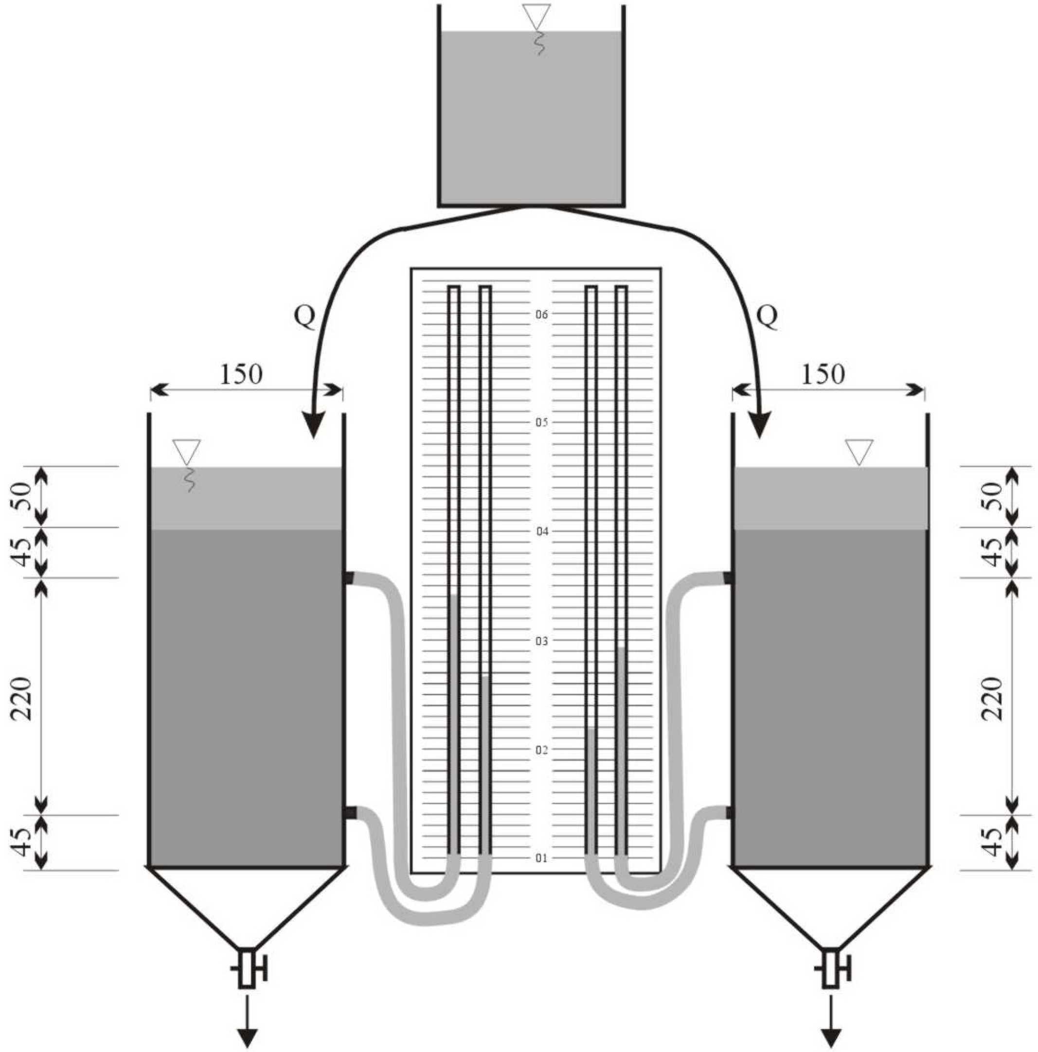
• K_s–hydraulic conductivity, m·s^−1;
• A–cross-section area of infiltration column, m^2;
• Δh_l–differenced in piezometer heights (head loss), m;
• L–length of the sample, m;
• V–seepage velocity, m·s⁻¹;
• Q–discharge of flow, m³·s⁻¹;
• I–hydraulic gradient;

Hydraulic conductivity was calculated using measurements made in the infiltration column. Additionally, relevant values of hydraulic conductivity were calculated, using well-known formulae based on physical parameters of the investigated soils. The first was the Hazen Formula in the form presented by Lange [20] where value of hydraulic conductivity also depends on porosity:

$$K_s=\left[400+40\cdot \left(n-26\right)\right]\cdot d_{10}^2$$

(3)

where,

• K_s–hydraulic conductivity, m·d⁻¹;
• d₁₀–effective grain size, mm;
• n–porosity, %.

The sand mine specification indicated d₁₀ as 0.1 mm, however, the d₁₀ estimated using sieving analysis was 0.08 mm on average. Taking into consideration this divergence (related probably to measurement precision) the d₁₀ value was approximated to 0.1 mm.

Hydraulic conductivity was also calculated using the USBR Formula as follows:

$$K_s=0.36\cdot d_{20}^{2.3}$$

(4)

where,

• K_s–hydraulic conductivity, cm·s⁻¹;
• d₂₀–effective grain size, mm.

2.3. Scale Effect-Free Laboratory Method Conducted in Controlled Conditions

2.3.1. Research Set-Up Description

Measurements were conducted on a research set-up_presented in Figure 2. The front sidewall of the tank was built out of a transparent plexiglass. The tank bottom with a centrally designed outflow was covered by a 0.1 m layer of gravel. The tank was filled with the investigated soil with a density corresponding to natural occurrence. After filling, at the soil surface a hole had been prepared according to the Amoozegar [21] instruction. Only one half of the hole of diameter of 0.15 m and depth 0.30 m was created at the transparent wall to observe water level and streamlines. The wall of the hole was protected against collapse by a brass mesh screened by a fabric filter [22]. Water used for the experiments was deaerated, as a direct application of tap water in this type of research may give the wrong results [23].

Figure 2. Scheme of the research set-up of the scale effect-free laboratory method.

Figure 2. Scheme of the research set-up of the scale effect-free laboratory method.

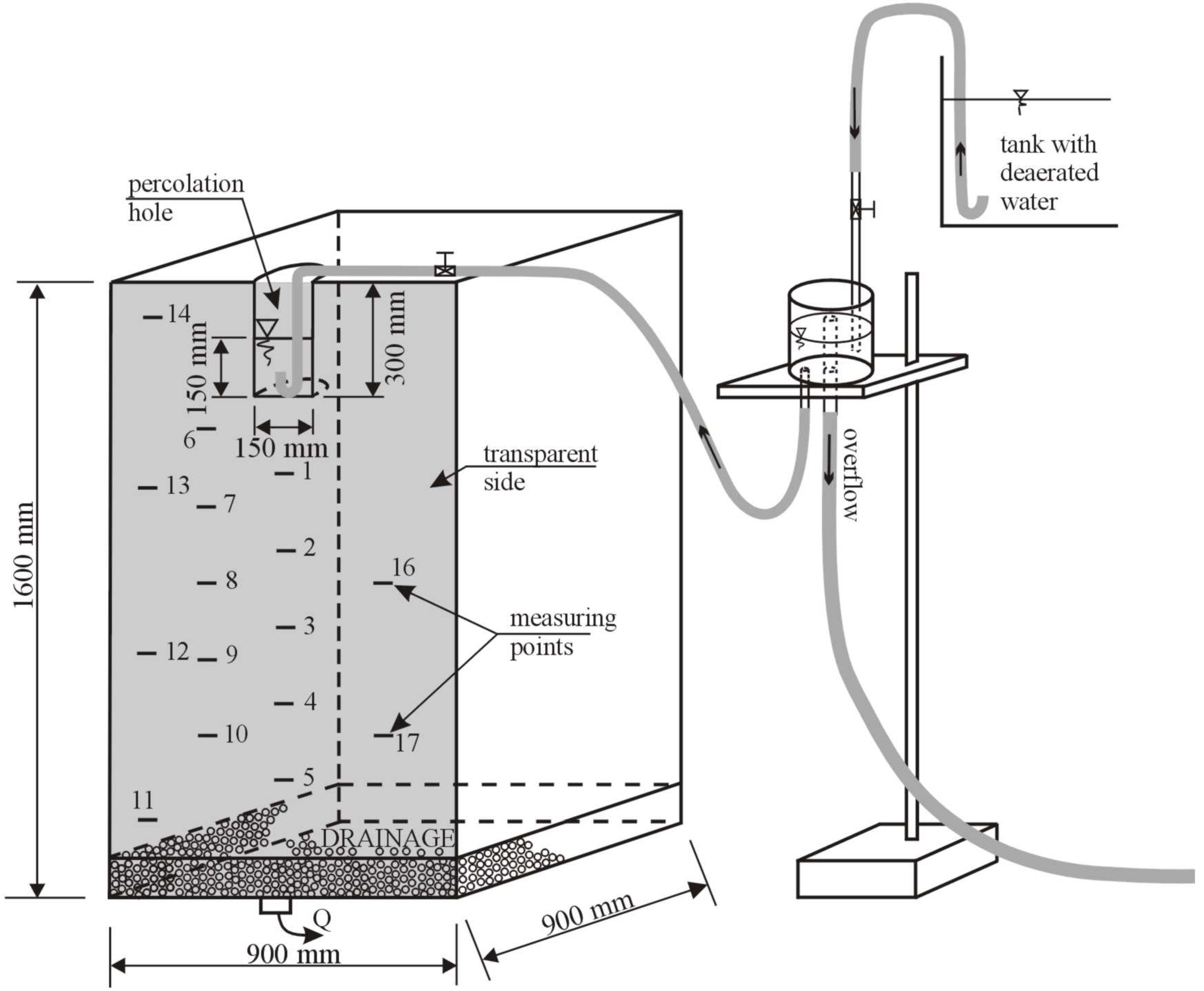
2.3.2. Calculations of Hydraulic Conductivity

Soil saturation was measured using the TDR method (Time Domain Reflectometry). During and after full saturation, percolation tests were conducted according to schedule. Two kinds of tests were used. The first consisted of maintaining a constant level of water equal to 0.15 m in the hole (steady-state condition). The second was a falling head test, where the time taken to the drop of water level from 0.15 m to zero (bottom) was recorded in each test. Calculations of hydraulic conductivity in falling head tests were conducted using the Van Hoorn equation [1]:

$$K_s=1.15r\frac{\log \left(H_0+\frac{r}{2}\right)-\log \left(H_1+\frac{r}{2}\right)}{t}$$

(5)

where,

• H₀–initially water level in the hole, m;
• H₁–final water level in the hole, m;
• r–radius of the hole, m;
• t–water falling time, s.

The above-presented equation is used to calculate the value of hydraulic conductivity in American tests known as the inversed auger hole method. In the French literature, this test is known as the Porchet method [12].

In steady-state tests the values of hydraulic conductivity were obtained by the Glover equation [24]. In a steady-state condition for a hole of cylindrical shape it holds:

$$K_s=Q\cdot \frac{{\sinh }^{-1}\left(\frac{H}{r}\right)-{\left[{\left(\frac{r}{H}\right)}^2+1\right]}^{\frac{1}{2}}+\left(\frac{r}{H}\right)}{2\cdot \pi \cdot H^2}$$

(6)

where,

• K_s–hydraulic conductivity, m·s⁻¹;
• Q–quantity water needed to hold a constant water level at H, m³·s⁻¹;
• H–constant water level in the hole, m.

In this paper additionally, the Philip equation was used to estimate hydraulic conductivity [24]:

$$K_s=\frac{\text{Q}}{C_p\cdot r^2}$$

(7)

$$C_p={\left(\frac{H^2}{r^2}-1\right)}^{\frac{1}{2}}\cdot \left\{\frac{4.117\cdot \left(\frac{H}{r}\right)\cdot \left(1-\frac{r^2}{H^2}\right)}{\ln \left[\frac{H}{r}+{\left(\frac{H^2}{r^2}-1\right)}^{\frac{1}{2}}\right]-{\left(1-\frac{r^2}{H^2}\right)}^{\frac{1}{2}}}+\frac{\left(8.056+5.034\cdot \frac{r}{H}\right)}{a\cdot r\cdot \ln \left[\frac{H}{r}+{\left(\frac{H^2}{r^2}-1\right)}^{\frac{1}{2}}\right]}\right\}$$

(8)

where,

C_p-factor, which depends on the shape of the hole, and takes into consideration both saturated and unsaturated components of water flow around the auger hole.

This equation allows to calculate the value of hydraulic conductivity for both saturated and unsaturated flow of water out of the hole. Coefficient a must be determined independently or to be estimated for a given type of soil from values reported by Erlic but presented by Amoozegar [21]. The a depends on the type of soil, as follows:

• a = 1–compacted clays;
• a = 4–unstructured fine-textured soils;
• a = 12–most structured soils from clays to loam and unstructured medium and fine sand and sandy loam;
• a = 36–coarse and gravelly sands.

3. Results and Discussion

Laboratory Measurements

Hydraulic conductivity was calculated using measurements made in the infiltration column. The results for a water temperature of 10 °C are presented in Table 2. Additionally, relevant values of hydraulic conductivity were calculated using the Hazen and the USBR formulae.

Table 2. Results of hydraulic conductivity obtained by different methods.

Soil type	Method	Mean value of K10	N number of measurements	LTAR *	Percentage variation comparing to IC
		(m·d−1)	-	(cm·d−1)	%
fine sand	IC	0.80 ± 0.01	85	1.79
	FHM	11.66 ± 0.11	45	3.60	101%
	CHM	2.03 ± 0.03	47	2.15	20%
	CHM a = 4	0.83 ± 0.01	47	1.80	1%
	Hazen	5.9	-	2.85	59%
	USBR	3.4	-	2.44	36%
medium sand	IC	1.93 ± 0.12	25	2.13
	FHM	7.65 ± 0.57	104	3.09	45%
	CHM	0.90 ± 0.03	31	1.83	−14%
	CHM a = 36	0.90 ± 0.03	31	1.83	−14%
	Hazen	12.5	-	3.70	73%
	USBR	7.7	-	3.10	45%
coarse sand	IC	5.27 ± 0.1	102	2.75
	FHM	6.02 ± 0.39	147	2.86	4%
	CHM	2.46 ± 0.08	295	2.25	−18%
	CHM a = 36	2.55 ± 0.09	295	2.13	−23%
	Hazen	40.8	-	6.57	139%
	USBR	19.5	-	4.47	62%

Notes: Not measured; ** LTAR is calculated using the formula presented by Laak-scale effect-free laboratory tests conducted in controlled conditions.

Table 2. Results of hydraulic conductivity obtained by different methods.

Soil type	Method	Mean value of K10	N number of measurements	LTAR *	Percentage variation comparing to IC
		(m·d−1)	-	(cm·d−1)	%
fine sand	IC	0.80 ± 0.01	85	1.79
	FHM	11.66 ± 0.11	45	3.60	101%
	CHM	2.03 ± 0.03	47	2.15	20%
	CHM a = 4	0.83 ± 0.01	47	1.80	1%
	Hazen	5.9	-	2.85	59%
	USBR	3.4	-	2.44	36%
medium sand	IC	1.93 ± 0.12	25	2.13
	FHM	7.65 ± 0.57	104	3.09	45%
	CHM	0.90 ± 0.03	31	1.83	−14%
	CHM a = 36	0.90 ± 0.03	31	1.83	−14%
	Hazen	12.5	-	3.70	73%
	USBR	7.7	-	3.10	45%
coarse sand	IC	5.27 ± 0.1	102	2.75
	FHM	6.02 ± 0.39	147	2.86	4%
	CHM	2.46 ± 0.08	295	2.25	−18%
	CHM a = 36	2.55 ± 0.09	295	2.13	−23%
	Hazen	40.8	-	6.57	139%
	USBR	19.5	-	4.47	62%

Notes: Not measured; ** LTAR is calculated using the formula presented by Laak-scale effect-free laboratory tests conducted in controlled conditions.

During research using the FHM in gravel and medium sand higher variations of the results were noted. Infiltration rates were found to be gradually decreasing during percolation tests.

The results of hydraulic conductivity obtained using the CHM showed a relatively low variation.

In the Philips equations, the parameter a was calculated using capillary rise measurements (h_k = 0.48 m) for fine sand. Assuming that the value of capillary rise is equal to the matrix potential the latter was calculated as a reciprocal of a, as follows [25]:

$$a=2{\left|\psi \right|}^{-1}=2h_k^{-1}$$

(9)

where,

• h_k–capillary rise in m H₂O;
• ψ–matrix potential m H₂O.

The value of a calculated using the Equation (9) a = 4.17 was close to the assumed value of the parameter (a = 4.0). In the calculation of a, the value was estimated and based on literature data. In the case where capillary rise is less then about 6 cm the value of a being equal to 36 has been found to be correct. Calculations of hydraulic conductivity in fine sand using Glover equations, comparing to those which neglect capillary rise, gave overestimated results.

The results of hydraulic conductivity obtained by empirical formulae based only on grain size distribution should be treated carefully, because the formulae are oversimplified. The results can be only used as a preliminary assessment of hydraulic conductivity.

Analysis of variance was completed with a significance level set on α = 0.05 confirmed significant differences in the compared tests. Therefore, it was important to conduct post hoc tests that can explain which values were responsible for rejecting the null hypothesis. The Tukey method was chosen to find which means are significantly different from one another. This test compare every group mean with every other group mean and typically incorporate some method of controlling for Type I errors.

Although Pedescol [26] did not explain the obtained result, the author reported that hydraulic conductivity of gravel soil obtained using the falling head method was about 38% higher than that obtained using a constant head method. However, the results of hydraulic conductivity obtained by both methods in a coarse sand were not significant (p < 0.05) despite the fact that the mean value estimated by the falling head method was several times higher than that obtained using the constant head method.

Comparison of hydraulic conductivities obtained by the falling head method and constant head method confirmed significant differences in the parameter (p < 0.05) between investigated soils obtained earlier by the author [27]. Comparable results were obtained by Spychała and Nieć [28], values obtained using the FHM test were higher than using CHM in the same conditions (geo-textile supplied with wastewater) but the difference was not as high (0.057 m/d and 0.047 m/d, respectively).

For fine and medium sand (most common soil types in practice) the relatively small values of the variation coeffcient (20% for fine sand and −14% for medium sand) for the 47 and 31 measurements respectively were made.

For the same types of soil the impact of differences between column measurements and constant water head test (CHM) measurement mean values on longterm acceptance rate (LTAR) [1] were relatively small. The hydraulic coefficient measurement points were located on the plotted LTAR function line (Figure 3). The significant differences in results for the same type of ground but using different methods (CHM, CHM-a and FHM) can be observed. These differences in hydraulic coefficient values implicates much smaller differences in LTAR values.

The best agreements were given by the method of constant head measurement for the calculation of hydraulic conductivity using the Glover equation, which gave similar results obtained, using the Philip equation for a parameter (which was equal to 36) as presented in Table 2. The differences between both variants of this test (without and with regard to capillary rise), for all types of sand, and infiltration column mean values were lower than 25%.

Figure 3. The hydraulic coefficient measurement points plotted on the LTAR function line.

Figure 3. The hydraulic coefficient measurement points plotted on the LTAR function line.

Taking into consideration that even filter column tests values were relatively highly differentiated (about 16%–31%) it seems that the differences between CHM test values and infiltration column mean values of about 20%–25% could be accepted. Values obtained from the CHM test were acceptable for medium and coarse sand (−14% and −18%, respectively) but less acceptable for fine sand (20%). The values with a minus sign mean that assessed hydraulic loading is lower than probably more certain values obtained from an infiltration column test. This is the reason that a potentially designed system will have a surface area of about 20% larger than optimal. From a practical point of view the 20% is a relatively small value and designing a larger surface area system gives some security margin, allowing for a decrease in clogging risk. In the case of fine sand the CHM-a test is preferred by authors for applications in practice than the CHM test, as it gives results in the long-term acceptance rate (calculated and based on the hydraulic coefficient) overestimated in comparison to the infiltration column. The value is not high but the sign is adverse due to the resulting smaller infiltration surface area than optimal (calculated based on infiltration column measurement). The difference between CHM-a test mean values and infiltering column test measurement values has the same sign but is very small—1% only, so it can be assumed that a measurement using this test is almost optimal. Taking this into consideration the authors of this paper suggest using CHM tests for medium and coarse sand and CHM-a for fine sand, or the CHM-a test for all types of soil.

For medium and coarse sandy soils (medium are the most common as a system location) the underestimation of calculated LTAR based on CHM test determination gives 14%–18% value of system infiltration surface area. In Poland the full cost of the most common type of on-site wastewater system (septic tank with soil absorption system in sandy soil for one four-person family) is about 2,000 EUR and soil absorption systems cost is about a half of the total cost (1,000 EUR). The cost of SAS designed systems, based on CHM in comparison to those designs based on real hydraulic conductivity value, is up to 7%–9% of total higher than on-site wastewater plant cost. This relatively low cost (70–90 EUR) gives some security value of infiltration surface area (14%–18%), preventing the system from clogging. For large surface area systems other methods or apparatuses should be recommended and used to determine K in the field—e.g., infiltrometers.

The FHM and well-known equations are not recommended by the authors for soil permeability and infiltration systems assessment due to the high difference compared to infiltration columns measurement results. The above can be used, however, for investigations of particular factors and their impact on soil permeability, indicating, e.g., wastewater solids [29].

4. Conclusions

Based on this study the following conclusions can be drawn:

• the differences in long-term acceptance rate values were about one magnitude smaller than differences in the hydraulic coeffcient (Figure 3), which is related to plotted function line slope;
• the research on medium and coarse sand showed that a similar result for hydraulic conductivity to that obtained from infiltration columns, which can be obtained using constant head tests; for the same types of soil the impact of difference between column measurements and constant water head test (CHM) measurement mean values on long-term acceptance rate value were relatively small–up to 14%–18%;
• studies conducted in fine sand confirmed a good convergence of hydraulic conductivity, using the infiltration column with constant head tests when the value of hydraulic conductivity is calculated with regard to capillary rise-the best agreements were given by the method of constant head measurement for the calculation of hydraulic conductivity, using the Philip equation for a parameter of 4;
• In the authors’ opinion the CHM tests measurements are acceptable for small systems (e.g., one family household). This test gives some overestimation, however it can be treated as a security factor preventing clogging risk. For calculating LTAR for low permeable soils (fine sand) the authors of this paper suggest using the CHM-a test where the unsaturated flow of water (common in small grain and pore diameter soils) can be determined thanks to a capillary rise determined by the test. For large surface area systems other, more precise methods or tests should be used to determine K in the field, e.g., infiltrometers;
• the cost of SAS designed based on CHM in comparison to designed based on real hydraulic conductivity value is higher up to 7%–9% of total on-site wastewater plant cost only;
• the result of hydraulic conductivity obtained in the falling head test can be overestimated due to the higher value of hydraulic gradient than unity assumed in development of the calculation formulae;
• the authors of this paper suggest using CHM-a especially for low permeable soils (e.g., fine sand) where the unsaturated flow of water occurs with regard to capillary rise so as to calculate hydraulic load as a LTAR.

References

- Laak, R. Subsurface Soil System. In Wastewater Engineering Design for Unsewered Areas; Technomic Publishing Company: Lancaster, PA, USA, 1986. [Google Scholar]
- Amoozegar, A. Report No.316, Impact of Wastewater Quality on the Long-Term Acceptance Rate of Soils for On-Site Wastewater Disposal Systems; WRRI Project No. 70140; Water Resources Research Institute of the University of North Karolina, North Carolina State University: Raleigh, NC, USA, July 1998. [Google Scholar]
- Beal, C.D.; Gardner, E.A.; Kirchhof, G.; Menzies, N.W. Long-term flow rates and biomat zone hydrology in soil columns receiving septic tank effluent. Water Res. 2006, 40, 2327–2338. [Google Scholar]
- Radcliffe, D.E.; West, L.T. Spreadsheet for converting saturated hydraulic conductivity to long-term acceptance rate for on-ste wastewater systems. Soil Surv. Horiz. 2009, 50, 20–24. [Google Scholar]
- Pedescoll, A.; Uggetti, E.; Llorens, E.; Granés, F.; García, D.; García, J. Practical method based on saturated hydraulic conductivity used to assess clogging in subsurface flow constructed wetlands. Ecol. Eng. 2009, 35, 1216–1224. [Google Scholar]
- Scott Purdy; Vector Engineering Inc.; Joel Peters; Vector Chile Ltda. Comparison of Hydraulic Conductivity Test Methods for Landfill Clay Liners. In Proceedings of the Beacon Conference “Sanitary Landfills for Latin America”, Buenos Aires, Argentina, 8–10 March 2004.
- Sobieraj, J.A.; Elsendbeer, H.; Vartessy, R.A. Pedotransfer functions for estimating saturated hydraulic conductivity: Implications for modeling storm flow generation. J. Hydrol. 2001, 251, 202–220. [Google Scholar]
- Islam, N.; Wallander, W.W.; Mitchell, J.P.; Wicks, S.; Howitt, R.E. Performance evaluation of methods to the estimation of soil hydraulic parameters and their suitability in a hydrologic model. Geoderma 2006, 134, 135–151. [Google Scholar]
- Ghanbarian-Alavijeh, B.; Liaghat, A.M.; Sohrabi, S. Estimating saturated hydraulic conductivity from soil physical properties using neural networks model. World Acad. Sci. Eng. Technol. 2010, 4, 108–113. [Google Scholar]
- Slichter, C.S. Theoretical Investigations of the Motion of Ground Waters; 19th Annual Report, Part II; U.S. Geological Survey: Lei Sidui, VA, USA, 1899. [Google Scholar]
- Aronovici, V.S. The mechanical analysis as an index of subsoil permeability. Soil Sci. Soc. Am. J. 1947, 11, 137–141. [Google Scholar]
- Oosterbaan, R.J.; Nijland, H.J. Determining the saturated hydraulic conductivity. In Drainage Principles and ApplicationsILRI Publication 16, 2nd ed.; Ritzema, H.P., Ed.; ILRI Publication: Wageningen, the Netherlands, 1994. [Google Scholar]
- De Ridder, N.A.; Wit, K.E. A comparative study on the hydraulic conductivity of unconsolidated sediments. J. Hydrol. 1965, 3, 180–206. [Google Scholar]
- Odong, J. Evaluation of empirical formulae for determination of hydraulic conductivity based on grain-size analysis. Available online: http://www.engineerspress.com/pdf/IJAE/2013-01/a1%20_IJAE-133101_.pdf (accessed on 18 September 2014).
- Vuković, M.; Soro, A. Determination of Hydraulic Conductivity of Porous Media from Grain-size Composition; Water Resources Publications: Littleton, CO, USA, 1992; p. 83. [Google Scholar]
- Spychalski, M.; Kaźmierowski, C.; Kaczmarek, Z. The possibilities of indirect filtration coefficient assessment in soil. Polski Towarzystwo Geologiczne Oddział w Poznaniu 2004, Tom XIII, 48–56. (In Polish) [Google Scholar]
- Bouma, J. Unsaturated flow during soil treatment of septic tank effluent. J. Environ. Eng. 1975, 101, 967–983. [Google Scholar]
- Kropf, F.W.; Laak, R.; Healy, K.A. Equilibrium operation of subsurface absorption systems. J. Water Pollut. 1977, 49, 2007–2016. [Google Scholar]
- Beach, D.; McCray, J.; Lowe, K.; Siegrist, R. Temporal changes in hydraulic conductivity of sand porous media biofilters during wastewater infiltration due to biomat formation. J. Hydrol. 2005, 311, 230–243. [Google Scholar]
- Lange, O.K. Basic Hydrogeology (Osnovi Gidrogeologii); Moskovskii Gosudarstvenii Univerzitet: Moscow, Russia, 1958. (In Russian) [Google Scholar]
- Amoozegar, A. Comparison of saturated hydraulic conductivity and percolation rate: Implication for designing septic system. In proceedings of Symposium on the Site Characterization and Design of On-Site Septic Systems, New Orleans, LA, USA, 16–17 January 1997.
- Bagarello, V.; Giordano, G. Comparation of procedures to estimate steady flow rate in field measurement of saturated hydraulic conductivity by the Guelph Permeameter method. J. Agric. Eng. Res. 1999, 74, 63–71. [Google Scholar]
- Hayashi, M.; Quinton, W.L. A Constant-head well permeameter method for measuring field-saturated hydraulic conductivity above impermeable layer. Can. J. Soil Sci. 2004, 84, 255–264. [Google Scholar]
- Bronders, J. Field and Laboratory Measurements to Determine Hydraulic Conductivity; Faculty of Applied Science Laboratory of Hydrology, Free University Brussels: Brussels, Belgium, 1991. [Google Scholar]
- Elrick, D.E.; Reynolds, W.D.; Tan, K.A. Hydraulic conductivity measurements in the unsaturated zone using improved well analyses. Ground Water Monit. Remediat. 1989, 9, 184–193. [Google Scholar]
- Pedescoll, A.; Samo, R.; Romero, E.; Puigagut, J.; Garcia, J. Reliability, repeatability and accuracy of the falling head method for hydraulic conductivity measurements under laboratory conditions. Ecol. Eng. 2011, 37, 754–757. [Google Scholar] [CrossRef]
- Nieć, J. Comparison of hydraulic conductivity determination methods for wastewater drainage. Seria Melior. Inż. Środ. 2005, 26, 293–304. (In Polish) [Google Scholar]
- Spychała, M.; Nieć, J. Impact of septic tank sludge on filter permeability. Environ. Prot. Eng. 2013, 39, 77–89. [Google Scholar]
- Spychała, M.; Nieć, J.; Pawlak, M. Preliminary study on filamentous particle distribution in septic tank effluent and their impact on filter cake development. Environ. Technol. 2013, 34, 2829–2837. [Google Scholar]
© 2014 by the authors; licensee MDPI, Basel, Switzerland. This article is an open access article distributed under the terms and conditions of the Creative Commons Attribution license (http://creativecommons.org/licenses/by/3.0/).
Share and Cite
Nieć, J.; Spychała, M. Hydraulic Conductivity Estimation Test Impact on Long-Term Acceptance Rate and Soil Absorption System Design. Water 2014, 6, 2808-2820. https://doi.org/10.3390/w6092808
Nieć J, Spychała M. Hydraulic Conductivity Estimation Test Impact on Long-Term Acceptance Rate and Soil Absorption System Design. Water. 2014; 6(9):2808-2820. https://doi.org/10.3390/w6092808
Chicago/Turabian StyleNieć, Jakub, and Marcin Spychała. 2014. "Hydraulic Conductivity Estimation Test Impact on Long-Term Acceptance Rate and Soil Absorption System Design" Water 6, no. 9: 2808-2820. https://doi.org/10.3390/w6092808