Next Article in Journal
Improved Energy Recovery by Anaerobic Grey Water Sludge Treatment with Black Water
Previous Article in Journal
The Energy Efficiency of Hot Water Production by Gas Water Heaters with a Combustion Chamber Sealed with Respect to the Room
 
 
Correction published on 25 September 2014, see Water 2014, 6(9), 2847-2848.
Article

Principal Component and Multiple Regression Analyses for the Estimation of Suspended Sediment Yield in Ungauged Basins of Northern Thailand

by
Piyawat Wuttichaikitcharoen
* and
Mukand Singh Babel
Water Engineering and Management Program, School of Engineering and Technology, Asian Institute of Technology, P.O. Box 4, Klong Luang, Pathumthani 12120, Thailand
*
Author to whom correspondence should be addressed.
Water 2014, 6(8), 2412-2435; https://doi.org/10.3390/w6082412
Submission received: 4 May 2014 / Revised: 21 July 2014 / Accepted: 29 July 2014 / Published: 12 August 2014

Abstract

:
Predicting sediment yield is necessary for good land and water management in any river basin. However, sometimes, the sediment data is either not available or is sparse, which renders estimating sediment yield a daunting task. The present study investigates the factors influencing suspended sediment yield using the principal component analysis (PCA). Additionally, the regression relationships for estimating suspended sediment yield, based on the selected key factors from the PCA, are developed. The PCA shows six components of key factors that can explain at least up to 86.7% of the variation of all variables. The regression models show that basin size, channel network characteristics, land use, basin steepness and rainfall distribution are the key factors affecting sediment yield. The validation of regression relationships for estimating suspended sediment yield shows the error of estimation ranging from −55% to +315% and −59% to +259% for suspended sediment yield and for area-specific suspended sediment yield, respectively. The proposed relationships may be considered useful for predicting suspended sediment yield in ungauged basins of Northern Thailand that have geologic, climatic and hydrologic conditions similar to the study area.

Graphical Abstract

1. Introduction

An estimation of suspended sediment yield is required for engineering practices that deal with improved land and water management practices in a river basin. The transport of sediment in rivers implies a series of negative effects, such as reservoir siltation and channel bed modification. Such effects may disturb the sediment balance in the basin. In particular, sediment that is eroded from sloping areas can accumulate in the river’s network, thereby affecting channel water conveyance [1]. Moreover, several problems due to soil erosion, such as the loss of fine and nutrient-rich topsoil that reduces land productivity, as well as the pollution of surface water bodies, are evident [2,3,4,5]. The study of erosion and sediment yield has long established itself as an important area of hydrological research due to the economic significance of the processes involved.
Similar to other developing Southeast Asian countries, land degradation is a major problem in Thailand. This problem manifests itself in terms of the soil structure and its fertility deterioration, in particular for sloping land [6]. Cultivation on sloping areas influences the environment in terms of siltation, flash floods, poor crop yields, etc. [7]. The estimation of sediment yield is required in planning and designing water resource development projects, especially for studying the feasibility of a dam or a barrage, assessing sediment budgets and examining the delivery of sediment and contaminants to the estuarine or ocean system, which also provides a valuable means of studying the denudation process [8]. However, sediment data is rarely available due to the lack of monitoring. Erosion and sediment transport are complex phenomena, and these processes are affected by several factors, such as climatic and geomorphological conditions, land use, etc.
The approaches employed to estimate sediment yield can be divided into four main groups [9], namely: (1) the soil erosion and sediment delivery approaches, wherein estimated soil erosion rates are factored by a sediment delivery ratio, which is often based on basin characteristics; (2) the physically-based and/or distributed basin modeling approaches, wherein the movement of water and soil is estimated in a distributed way throughout the basin; (3) the models relating sediment concentration or the load to the river flow, wherein measured sediment concentration data is related to river flow characteristics; and (4) empirical models based on broad basin and climate descriptors, wherein sediment yield equations are derived from known basin characteristics. The soil erosion and sediment delivery approaches are usually based on the Universal Soil Loss Equation (USLE) [10] and the concept of the sediment delivery ratio (SDR) [11]. Although many combinations of erosion and sediment delivery modelling are available [12,13,14,15,16], they still require calibration and, thus, cannot be transferred from the study area to other catchments and environments. Moreover, USLE cannot be applied easily to non-agricultural land uses or to areas outside of the range of the original development and application [9].
The physically-based model describes the physical processes involved in the flow and transport of sediment, and these processes use the laws of the conservation of mass, momentum and sediment transport to explain the inherent processes; however, the physically-based model requires extremely onerous input data. When the input data is scarce, the large number of involved parameters may cause significant uncertainty in soil erosion estimates [1]. Furthermore, the simulation of sediment transport at the basin scale is still computationally very expensive. The models relating sediment concentration or load to river flow are most commonly used in practice. These models assume that river flow, rather than sediment supply, is the dominant factor in sediment yield. However, such models also require a large amount of data to give realistic estimates of long-term average annual sediment yield. This approach is based on “what has happened” rather than “what may happen”. Understanding sediment supply and transport processes is required to extrapolate their potential consequences during unmonitored future climate and/or land-use scenarios. The empirical model is based on limited knowledge of the processes and relies on the data describing input and output behavior. This method, however, is able to make abstractions and generalizations of the process and often complements the physically-based model [17].
Several authors have shown the effectiveness of statistical relationships, which allow one to estimate river sediment transport depending on easily available geomorphologic, hydrological and climatic parameters [1,18,19,20,21,22,23,24,25,26,27,28,29,30,31,32,33]. Sediment yield is controlled by factors that control erosion and sediment delivery, including local topography, soil properties, climate, vegetation cover, catchment morphology, drainage network characteristics and land use [26,28]. Langbein and Schumm [32] studied the relationship between mean annual precipitation and sediment yield in the United States, while Walling and Webb [31] concluded that no simple relationship exists between climate and sediment yield, because climate’s effect on sediment load is very complex. Anderson [33] proposed three major groups of explanatory variable as being involved in relating sediment yield to watershed variables. These are the hydrologic event variables, the watershed conditions and land use variables, as well as the inherent watershed variables, such as area, geology and physiography. He also mentioned that sediment measuring device and its efficiency is also important in having accurate sediment measurements. Bray and Xie [29] identified six categories of variables that can be related to the processes associated with the generation and delivery of suspended sediment to the basin outlet in Canada, which are hydroclimatic conditions, basin topographic features, land surface features, soil characteristics, channel network features and human activities. Ciccacci et al. [30] and Grauso et al. [1] investigated the correlation between the sediment yield and some geomorphologic, hydrological and climatic parameters in Italy. They found a significant relationship between average yearly sediment yield per unit watershed area and the drainage density. Restrepo et al. [23] developed a multiple regression model for estimating the sediment yield in a South American watershed. They reported six catchment variables that predict sediment yield, including runoff, precipitation, precipitation peakedness, mean elevation, mean water discharge and relief, while the mean annual runoff is the dominant control factor. Syvitski and Milliman [22] provided a description of factors influencing the estimation of sediment loads from rivers, which are drainage area size, basin relief, geologic condition, climate and vegetation cover. They successfully estimated the long-term flux of sediment delivered by rivers to the coastal zone (488 global rivers) by the BQART model, which is influenced by geomorphic and tectonic characteristics, geography, geology and human activities. Recently, Cohen et al. [19] introduced a comprehensive global fluvial sediment predictor named WBMsed (Water Balance Model with sediment), a distributed global-scale riverine sediment flux model. The major important inputs for the model are anthropogenic factors, ice cover, lithology, reservoir sediment trapping, drainage area size, maximum basin relief, daily temperature and daily discharge.
The statistical method for reducing a large number of interrelated variables into a smaller number of dominant variables is called principal components analysis (PCA) and has been used in many areas of scientific research [17,34,35,36,37,38,39,40]. Recently, Tayfur et al. [41] investigated sediment load prediction and generalization from the laboratory scale to the field scale using principle component analysis (PCA) in conjunction with data-driven methods of artificial neural networks and genetic algorithms. In spite of these several uses, there is a disadvantage to PCA: the interpretability of the second and higher components may be limited. For this reason, Varimax rotation is applied to the PCA’s solution to enhance the interpretability of the components by maximizing a simple structure. An alternative rotational approach is known as the independent component analysis (ICA) [42,43,44], which finds a linear representation of non-Gaussian data, so that the components are statistically independent. Westra et al. [44] report that the PCA and Varimax rotations provide fairly accurate interpretations for global and local phenomena, respectively, while the interpretability of ICA results appears to be less successful.
The objectives of this study are to propose a complementary methodology that can be used in the prediction of suspended sediment yield in an ungauged basin (i.e., one where the river flow data is unavailable) based on a data-driven modeling approach. The use of the PCA with Varimax rotation to identify the key factors affecting sediment yield and the use of multiple regression analysis to establish the relationships between suspended sediment yield and the basin’s characteristics in terms of geomorphology and climate are also investigated.

2. Study Area

The study basin covers an area of 102,636 km
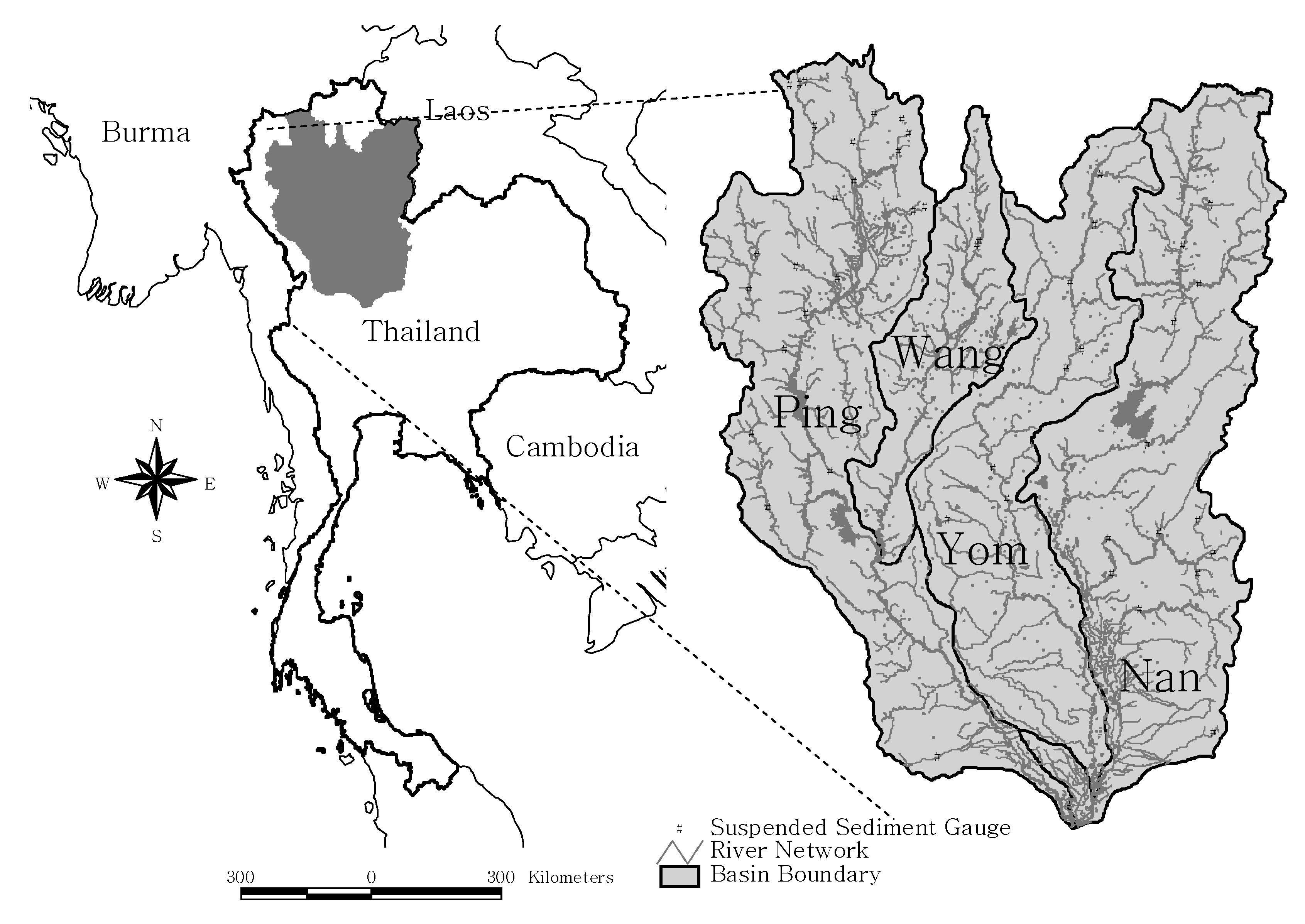
2 of Ping, Wang, Yom and Nan river basins in Northern Thailand. It is located between 15°30′ N and 20°00′ N latitudes and 98°00′ E and 101°30′ E longitudes (Figure 1). The Ping, Wang, Yom and Nan rivers are the main tributaries of the Chao Phraya River, the most important river of Thailand. These four tributaries originate from the Phi Pannam Mountain and course through mountainous areas before merging with each other in the alluvial plains of the Nakhon Sawan Province to form the Chao Phraya River.
Figure 1. The study area showing the locations of suspended sediment gauging stations.
Water 06 02412 g001
The study area is mountainous, with agriculturally productive valleys. The Ping, Wang, Yom and Nan rivers travel from north to south. The climate of the study area is dominated by seasonal monsoons. The rainy season that lasts from May to October is influenced by the southwest monsoon from the Indian Ocean and the depressions originating in the Pacific Ocean. The average monthly temperature ranges from 15 °C in December to 40 °C in April, except in high altitude locations. The study area can be classified as a tropical rainforest with high biodiversity. The general description of the study area [45] is presented in Table 1.
Table 1. A general description of the study area.
Basin CharacteristicPingWangYomNan
Drainage area (km2)33,89610,79123,61634,331
Main river length (km)740460735770
Forest area (percent)73.6676.0749.6845.14
Mean annual discharge (m3·s−1)276.5951.26115.95381.07
Mean annual runoff (106 m3·yr−1)8725.301617.503656.6012,014.80
Mean annual rainfall (mm·yr−1)1125109911591241
No. of selected rain gauge stations45232334
No. of selected suspended sediment gauging stations221410
In terms of soil erosion, Alford’s report [46] on mountain watersheds informs us that the Chao Phraya river basin, in Northern Thailand, showed no evidence of a significant increase in sediment yield during the period extending from the late 1950s to the mid-1980s. However, the Northern region of Thailand is very vulnerable to soil erosion, due to its undulating topography, steep slopes and high rainfall. Due to rapid economic development and population growth in the area, the forest-covered land in this northern region decreased from 68.54% in 1961 to 54.27% in 2004 [47]. The most vulnerable area is steeply sloping land, which is under cultivation (more than 35% of sloping land). In recent times, human encroachment on forest areas in the upper part of the study area and land use changes with respect to agriculture have become problematic [48].

3. Framework of the Analysis

The overall study framework involves basin data collection, principal component analysis (PCA) and multiple regression analysis. The data used in the analysis were obtained from hydro-meteorological stations, topographic maps, soil maps and land use maps of the study area. PCA is employed to determine the most prominent variables, which are then used in multiple regression analysis. The details of the data compiled and the methodology employed are presented in the following sections.

3.1. Basic Data

3.1.1. Geomorphic Parameters

The topography of the study area was acquired as a 30-m digital elevation model (DEM) from the Geo-Informatics and Space Technology Development Agency (GISTDA). The 30-m DEM was aggregated to 150-m resolution. This aggregation was done for the further use of the DEM in the physically distributed watershed model, Distributed Hydrology Soil Vegetation Model (DHSVM) [49], in the next phase of this research, which will be published in the near future. The characteristics of each of the sub-basins within the study area were then derived using HEC-GeoHMS 10.1 [50]. These characteristics include basin area, basin perimeter, basin length, basin slope, main channel length, distance between the basin outlet and a point on the stream nearest to the centroid of the basin area, total channel length, drainage density, basin relief, relief ratio, basin elongation and basin circularity. Most of the extracted basin areas and river networks match well with the existing GIS maps published by the Department of Water Resources (DWR) [51]. It is worth noting that a few sub-basins could not be delineated in areas that are relatively plains, which create difficulties in delineating the river and basin boundary. The river network’s properties, namely the hierarchical anomaly index and the hierarchical anomaly density [1,21,30,52,53], were estimated based on the digitized river network derived from 1:50,000 topographical maps obtained from the Royal Thai Survey Department, which was satisfactorily compared to the existing river network [51]. To elaborate on the river network’s properties, let us assume G as the number of first order streams necessary to make a drainage network perfectly ordered in a binary tree-shaped structure with streams of order K flowing into streams of order K + 1, and N is the number of first order streams present in the drainage network. The hierarchical anomaly index (DA) is given by the ratio of G to N, while the hierarchical anomaly density (GA) is the ratio of G to the basin area in square kilometers. These two parameters express the organization degree of drainage networks. Ciccacci et al. [30] and Grauso et al. [21] provide more details of these two parameters.

3.1.2. Soil Properties

The soil map of the study area was drawn using the Soil Program software [54], which derives 5-min resolution (about 10 km) soil data from the World Inventory of Soil Emission Potentials (WISE) pedon database [55], developed by the International Soil Reference and Information Centre (ISRIC) and the FAO-UNESCO Digital Soil Map of the World [56]. In this study, the soil clay content as a percentage was extracted and used as the soil’s representative property.

3.1.3. Land Use

The digital land use map, obtained from the Land Development Department (LDD) of the Royal Thai Government, was employed in this study. It was derived from Landsat 5 satellite imagery with 30-m resolution and the ground truth survey of 2000–2003. The forest and agricultural areas were extracted from each of the sub-basins to represent the land cover property used in the analysis.

3.1.4. Hydro-Meteorological and Sediment Data

The daily suspended sediment yield data, observed at 37 gauging stations operated by the Royal Irrigation Department (RID) and the Department of Water Resources (DWR) of the Royal Thai Government, were obtained as presented in Table 2. Daily suspended sediment data were calculated using the Sediment-discharge rating curve technique. The rating curve is derived using at least 20 measurement points per year for each station. The United States standard sampling method and equipment e.g., depth integrating sampler (US DH-48, US DH-49 and US DH-59) or point integrating sampler (US-P-46, US-P-61, US-P-63 and US-P-50), are employed based on water depth and the accessibility of each measurement point [57]. The examples of sediment-discharge rating curve equations provided by RID for the year 2000 for Ping, Wang, Yom and Nan river basins are: QS = 4.8767 QW1.323 (R2 = 0.811, 32 observation points at P.65 for Ping), where QS is suspended sediment load in tons day−1 and QW is river discharge in m3·s−1; QS = 3.0996 QW1.39 (R2 = 0.945, 27 observation points at W.16A for Wang); QS = 6.0248 QW1.244 (R2 = 0.886, 63 observation points at Y.34 for Yom); and QS = 0.1792 QW1.9793 (R2 = 0.922, 31 observation points at N.42 for Nan); respectively. Since there are no existing water infrastructures upstream of the gauging stations, the data are free from the effects of regulating structures. The daily rainfall data, monitored by RID and the Thai Meteorological Department (TMD), were obtained from 125 stations located in the study area. Since land use data were available for 2000–2002, both sediment and rainfall data collected from 1995 to 2007 (based upon availability) were used in the study, assuming that the land use remains the same and that there are no major man-made changes taking place for the study data period.
The annual suspended sediment yield was calculated using the daily data for each of the selected sub-basins. Table 2 shows the general description of the suspended sediment gauging stations in this study. For climate characteristics, annual rainfall, wet season rainfall (May–October), dry season rainfall (November–April) and the precipitation concentration index [58] were estimated. The mean areal rainfall was estimated by the Thiessen polygon method using the ArcView ArealRain Extension [59]. In each of the sub-basins, the time series data—suspended sediment yield, annual rainfall, etc.—were averaged as long-term average data for further analysis. The glossary and summary statistics of the variables used in this study are given in Table 3.

3.2. Principle Component Analysis

Principal component analysis (PCA) was applied in this study to identify the factors influencing suspended sediment yield. The PCA is a method of data reduction that aims to identify a small number of derived variables from a larger number of original variables in order to simplify the subsequent analysis of the data [60,61]. Moreover, the PCA has been used in the present study as the preliminary step in the development of a prediction model [62]. The sequence of the main steps involved in the PCA, as applied by Halim et al. [38], were adapted and are described below:
(1)
Selection of a set of basin characteristics and meteorological indicators for the study area. The initial set consisted of 17 basin characteristics and 4 climate factors (Table 3).
(2)
Assessment of the suitability of data for the PCA using the Kaiser–Meyer–Olkin (KMO) measure of sampling adequacy [63] and Bartlett’s test of sphericity [64]. KMO tests the ratio of item correlations to partial item correlations. If the partials are similar to the raw correlations, it means that the item does not share much variance with other items. This is a necessary criterion, since PCA assumes that common factors are the source of variance for the variables under investigation. The range of KMO is from 0.0 to 1.0; however, the score of 0.50 is suggested as the minimum value for a good PCA [65]. Bartlett’s test of sphericity checks for the hypothesis that the correlation matrix is an identify matrix, which means that all of the variables are uncorrelated. The significance value for this analysis led us to reject the null hypothesis and conclude that there are correlations in the data set that are appropriate for the PCA. The score from Bartlett’s test of sphericity with significance at 95% (p < 0.05) is considered appropriate for the PCA [61]. In addition, Tabachnick and Fidell [66] also recommend that, for the PCA, the correlation matrix should show at least some correlations, with the correlation coefficient being greater than or equal to 0.30.
(3)
Determination of dominant factors. The PCA with Varimax rotation is performed to identify the principal components (PCs) or subsets from a larger data set. For selecting the dominant factors, Kaiser’s criterion or the eigenvalues rule, i.e., only components with eigenvalues of 1.0 or more are retained for further investigation [38,67,68], was employed.

3.3. Regression Analysis

The regression relationships between suspended sediment yield and the dominant factors obtained from the PCA, i.e., biophysical and climate factors, were established using Equation (1). In order to avoid the negative lower boundary of estimation, a logarithmic transformation was used. The regression coefficients were obtained by ordinary least squares linear regression on logarithms of response and predictor variables. Finally, a back-transformed relationship was obtained in the form [62]:
Y = β0X1β1X2β2Xpβp
where Y is the response variable (suspended sediment yield in this study), X1, X2, …, Xp are the predictor variables (the factors influencing suspended sediment yield) and β0, β1, β2, …, βp are constants derived by the multiple linear regression analysis. The most commonly used procedure for selecting the best regression equation is stepwise linear regression analysis (using an F probability of 0.05 for the selected factor), as described by Landau and Everitt [60], was performed using SPSS for Windows Release 11.5.
Generally, the size of the drainage area is an important factor for both suspended sediment yield and area-specific suspended sediment yield. The relationship between the size of the drainage area and suspended sediment yield is complicated by many other factors, such as rainfall, plant cover, texture of the sediment and land use [69]. In order to evaluate the effect of each dominant factor in predicting suspended sediment yield in various categories of basin sizes [70] and based on the available data, regression models were generated based on 4 groups of data: (1) 7 sub-basins with a drainage area of less than 100 km2 (small basins); (2) 15 sub-basins with a drainage area of more than 100 km2, but less than 1000 km2 (medium basins); (3) 8 sub-basins with a drainage area of more than 1000 km2 (large basins); and (4) all 37 sub-basins irrespective of drainage area size.
Table 2. List of suspended sediment gauging stations in this study.
No. *Station CodeStation Name or LocationData PeriodBasin Area ** (km2)Avg. Annual Rainfall (mm·yr−1)Avg. Annual Runoff (mm·yr−1)Avg. Annual Sediment (ton km−2·yr−1)
Ping
1060201Nam Mae Mae at Ban Mae Na ***1995–200747.54129248253.84
2060202Nam Mae Pam at Sop Huai Mae Mat (Down Stream)1995–2007205.631034295120.36
3060301Nam Mae Ngat at Ban Teen That1997–200785.2896953526.88
4060302Nam Mae Saluam at Ban Thung Ku1997–200743.65115228650.43
5060401Huai Mae Hat at Ban Na Mon1997–200475.02103635618.05
6060406Nam Mae Taeng at Ban San Pa Sak (Upstream)1997–2004875.05117029164.90
7060602Nam Mae Rim at Ban Nong Gai1995–2004163.35105330824.73
8060701Nam Mae Wan at Aban Mae Wan1998–200547.66129172860.96
9060704Huai Ma Klaing at Ban Pa Maing Pang Bong2000–20055.021425932122.34
10060804Nam Mae Sapok at Ban Mae Sapok (Upstream)1996–200636.41135235220.97
11060808Nam Mae Khan at Ban Piang1995–20071199.95131818153.82
12061202Nam Mae Mu at Ban Mae Mu1995–200667.10135037313.99
13061302Nam Mae Chaem at Bana Kong Kan1996–20072055.651152309134.58
14061501Nam Mae Tun at Ban Pa Kha1995–20071588.79995454140.61
15P14Nam Mae Chaem at Kaeng Ob Luang Chiang Mai2000–20053828.311256274216.25
16P24ANam Mae Klang at Pracha Uthit Chiang Mai1997–2005449.33105131649.58
17P35Khlong Khlung at Ban Pang Wai Kamphaeng1995–2001745.22140646873.51
18P4ANam Mae Taeng at Ban Sanmahaphon Chiang Mai1995–20071892.48116118044.84
19P56ANam Mae Ngat at Ban Sahakhon Chiang Mai2000–2007546.39108234655.33
20P64Nam Mae Tun at Highway Bridge Chiang Mai1997–2002494.51102141999.19
21P65Nam Mae Teang at Ban Muang Pog Chiang Mai1995–2001233.71104139845.81
22P70Nam Mae Taeng at Ban Huai Khrai Chiang Mai1997–2000173.141049324110.05
Wang
23W16ANam Wang at Ban Hai Lampang2000–20071330.071,29924374.91
Yom
24Y24Nam Pi at Highway Bridge Phayao1997–2005591.191,25123344.12
25Y26Nam Mae Mok at Ban Mae Phu Lampang1998–2006787.01122225313.93
26Y34Nam Mae Lai at Ban Mae Lai Phrae1997–2002333.23129530632.58
27Y36Mae Nam Khuan at Ban Pa Kha Phayao2000–2005851.54128544878.34
Nan
28N22Khwae Noi at Ban Yang Phitsanulok1997–20064648.481340443125.12
29N24Nam Khek at Ban Wang Nok Phitsanulok1998–20061816.701383524149.53
30N40Khwae Noi at Ban Nong Bon Phitsanulok1999–20044180.451420507156.74
31N42Nam Wa at Ban Hat Khao Nan1997–20022085.9113161013255.52
32N49Nam Yao at Highway Bridge Nan2000–2005157.661456986160.89
33N53Khlong Butsabong at Ban Huai Tum Phetchabun1999–2006100.781472577342.75
34N58Nam Fua at Ban Kok Muang Phitsanulok2001–2006296.531263437301.56
35N59Lam Nam Khan at Ban Na Chan Phitsanulok2001–2006404.371,336551186.64
36N63Nam Haeng at Highway Bridge Nan1997–2005739.961,11218770.46
37N69Nam Nan at Ban Na Thung Yai Phitsanulok2000–2004168.75122763396.81
Notes: * Stations No. 1 to 14 belong to Department of Water Resources (DWR), and those from No. 15 to 37 belong to Royal Irrigation Department (RID); ** the basin area is extracted from DEM; *** bold stations and data are not used in developing the regression model and are used for validating the developed model.
Table 3. Glossary and summary statistics for the sub-basin’s characteristics.
Sub-basin characteristicUnitDescriptionSub-basin range
95% l.l.*Median95% u.l.**
Basin characteristics
AApercentAgricultural area0.0116.4464.68
AREAkm2Basin area33.27449.334227.26
BC-Basin circularity0.1580.2710.395
BE-Basin elongation0.4840.7511.085
BLkmBasin length8.2026.0591.51
BPkmBasin perimeter37.05154.80570.45
BRmBasin relief374.901010.001680.80
BS-Basin slope0.0060.0230.089
DA-Hierarchical anomaly index0.2351.0252.341
DDkm−1Drainage density0.9451.6772.165
FApercentForest area33.1582.2097.64
GA-Hierarchical anomaly density0.170.941.96
LCkmDistance from basin outlet to a point on the stream nearest the centroid of the basin area6.5318.8385.81
MCLkmMain channel length10.9041.66175.77
RR-Relief ratio0.0110.0380.128
TCLkmTotal channel length54.67584.446168.68
TSCCpercentTop soil clay content24.5125.0727.20
Climate
ARmm·yr−1Annual rainfall992.481256.341457.77
DSRmm·yr−1Dry season rainfall113.17154.75195.10
PCI-Precipitation concentration index15.2916.7518.26
WSRmm·yr−1Wet season rainfall855.231106.341333.35
Sediment
ASSYton km−2·yr−1Area-specific suspended sediment yield13.9873.51305.67
SSYton yr−1Suspended sediment yield74930,232672,487
Notes: The overall data is 37 samples from 37 sub-basins; * lower limit; ** upper limit.

3.4. Model Validation

From the 37 samples (37 selected stations), 30 samples were used for the multiple regression model’s development, while the remaining 7 samples were randomly excluded, based on the drainage area size, for the validation of the model. Additionally, a method called the jack-knife technique [62] was applied to examine the validity of developed regression models. This technique is generally performed by excluding one sub-basin from the total sub-basins. After that, regression having the same form as that of the general model was fitted using the all-but-one sub-basins, and the suspended sediment yield (SSY) or area-specific suspended sediment yield (ASSY) of the left out sub-basin was estimated by the obtained regression model called the test model. The calculation procedure was repeated for all sub-basins, and the coefficient of determination of the test model was calculated. Furthermore, the Pearson product-moment correlation coefficient between the predicted SSY or ASSY from the general and test models was also calculated.

4. Results and Discussion

4.1. Factors Influencing Suspended Sediment Yield

In this study, prior to performing PCA, the suitability of data for analysis was assessed. There were 37 datasets of 23 variables consisting of 17 basin characteristics, four climate factors and two sediment related variables (Table 3). The cross-correlations among 23 variables are given in Table 4. The KMO score was 0.59 and Bartlett’s test of sphericity showed significance at 95%, which reasonably supports the factorability of the cross-correlation. Additionally, the correlation matrix showed many correlation coefficients to be above 0.30. Therefore, factor analysis could be applied to reduce the number of factors in this study.
The PCA results based on the correlation matrix analysis with Varimax rotation indicate six principal components with eigenvalues greater than 1.00, which correspond to an overall cumulative variance of 86.7%. The order of significance of these variables is determined by the magnitude of their eigenvalues, as presented in Table 5.
The different variables considered in the PCA and their factor loadings within their respective PCs are presented in Table 6. It shows that the high weighted variables (factor loading ≥ 0.60) for PC1 consist of the total channel length (TCL), basin area (AREA), main channel length (MCL), distance from the basin outlet to a point on the stream nearest to the centroid of the basin area (LC), basin perimeter (BP), suspended sediment yield (SSY), basin length (BL), hierarchical anomaly index (DA), and hierarchical anomaly density (GA). PC2 consists of wet season rainfall (WSR), annual rainfall (AR) and hierarchical anomaly density (GA). PC3 consists of basin slope (BS), relief ratio (RR) and basin circularity (BC). PC4 consists of agricultural area (AA), forest area (FA) and area-specific suspended sediment yield (ASSY). PC5 consists of the precipitation concentration index (PCI) and dry season rainfall (DSR). Lastly, PC6 has basin elongation (BE) as a variable with high loading. From PC1 and PC4, it was seen that the suspended sediment yield (SSY) corresponds to the basin size (AREA), whereas area-specific suspended sediment yield (ASSY) corresponds to such land cover characteristics as forest area (FA) and agricultural area (AA), which imply that forest cover can reduce the erosion rate.
In addition, from Table 6, basin relief (BR) and top soil clay content (TSCC) show less commonality than the others, with scores of 0.319 and 0.645, respectively. These numbers suggest that a substantial portion of the variable’s variances is not accounted for by these two factors, and these are considered as less closely related to other variables.
Table 4. Correlation matrix of the identified variables.
VariableAREABPBLBSMCLLCTCLDDBRRRBEBCTSCCFAAAARWSRDSRPCIGADASSYASSY
AREA1.000.970.82−0.470.930.930.99−0.330.12−0.490.09−0.62−0.07−0.210.210.230.090.26−0.030.470.780.920.29
BP 1.000.88−0.590.980.960.95−0.430.13−0.610.04−0.75−0.01−0.230.240.210.080.32−0.050.430.800.870.29
BL 1.00−0.570.940.920.85−0.290.24−0.61−0.32−0.69−0.06−0.010.020.11−0.010.25−0.050.600.840.780.29
BS 1.00−0.58−0.53−0.480.380.050.99−0.100.76−0.160.29−0.310.180.25−0.430.22−0.35−0.58−0.38−0.12
MCL 1.000.980.92−0.400.20−0.60−0.08−0.74−0.04−0.160.160.190.080.29−0.020.480.830.860.29
LC 1.000.91−0.390.24−0.55−0.14−0.70−0.04−0.140.150.230.110.230.020.470.810.850.27
TCL 1.00−0.230.12−0.500.03−0.59−0.09−0.140.150.160.020.24−0.060.560.790.910.28
DD 1.00−0.080.35−0.240.56−0.200.39−0.40−0.37−0.35−0.410.060.35−0.28−0.31−0.29
BR 1.000.07−0.32−0.05−0.120.11−0.100.090.13−0.060.250.070.190.15−0.04
RR 1.00−0.020.76−0.180.27−0.280.170.24−0.390.21−0.38−0.61−0.40−0.14
BE 1.000.100.01−0.470.460.01−0.020.41−0.24−0.30−0.150.010.04
BC 1.00−0.220.29−0.30−0.10−0.07−0.320.07−0.23−0.62−0.54−0.27
TSCC 1.00−0.130.090.120.190.32−0.21−0.30−0.17−0.100.17
FA 1.00−0.99−0.35−0.30−0.29−0.040.28−0.06−0.20−0.55
AA 1.000.320.270.290.05−0.270.070.210.55
AR 1.000.930.190.25−0.36−0.020.250.39
WSR 1.000.090.33−0.48−0.150.100.33
DSR 1.00−0.67−0.010.250.260.25
PCI 1.00−0.29−0.20−0.04−0.13
GA 1.000.740.480.07
DA 1.000.760.29
SSY 1.000.47
ASSY 1.00
Notes: Bold values indicate correlation coefficients above 0.30; Kaiser–Meyer–Olkin measure of sampling adequacy: 0.59; Bartlett’s test of sphericity: 1347.44; significance: 0.000.
Table 5. Principal components (PCs) for basin characteristic and climate factors.
PCsEigenvaluesVariance (%)Cumulative variance (%)
19.43936.03136.031
23.81712.60248.633
32.70612.06860.701
41.52710.88171.582
51.3958.48980.071
61.0606.64486.715
Table 6. Results of principal component analysis (Varimax rotated component matrix).
FactorEigenvectorsCommonalities
PC1PC2PC3PC4PC5PC6
AREA0.9550.087−0.1010.0870.009−0.1330.955
BP0.9310.099−0.2820.0770.023−0.0930.972
BL0.891−0.001−0.272−0.0450.0150.2580.937
BS−0.4270.2780.783−0.170−0.1370.0590.924
MCL0.9410.091−0.2790.024−0.0040.0180.972
LC0.9340.131−0.2450.004−0.0530.0510.955
TCL0.9620.002−0.0680.0600.029−0.0690.940
DD−0.244−0.5120.525−0.126−0.1090.2790.702
BR0.2140.242−0.024−0.255−0.3120.2270.319
RR−0.4480.2820.774−0.165−0.134−0.0210.924
BE−0.068−0.0040.0310.2960.270−0.8640.912
BC−0.562−0.0850.710−0.139−0.036−0.0960.858
TSCC−0.2330.335−0.4480.0370.4660.2420.645
FA−0.056−0.2030.231−0.8750.0190.2840.944
AA0.0650.179−0.2390.879−0.038−0.2850.948
AR0.1740.8680.1420.239−0.0220.0260.863
WSR0.0230.9150.0940.184−0.0820.0710.893
DSR0.2210.190−0.2730.0970.773−0.2640.836
PCI−0.0600.2680.0110.027−0.9030.0590.895
GA0.629−0.6120.137−0.0830.1180.3380.925
DA0.867−0.200−0.1840.0590.0860.1530.860
SSY0.9220.0980.0230.1840.0540.0030.896
ASSY0.2830.2470.0860.7450.2550.3170.869
Notes: Extraction method: principal component analysis, rotation method: Varimax with Kaiser normalization; bold values indicate highly correlated variables included in the PCs (>0.60); underlined values correspond to the first three highest factor loadings in the PCs.
To select prominent variables for subsequent regression analyses, the first three variables with the highest factor loadings and greater than 0.60 were selected as representative variables of each of the PCs. A threshold of 0.60 was used for identifying a reliable factor in this study [71]. Therefore, for PC1, the total channel length (TCL), basin area (AREA) and main channel length (MCL) were selected. For PC2, wet season rainfall (WSR), annual rainfall (AR) and hierarchical anomaly density (GA) were employed. For PC3, basin slope (BS), relief ratio (RR) and basin circularity (BC) were used. Agricultural area (AA) and forest area (FA) were extracted from PC4, whereas area-specific suspended sediment yield (ASSY) was considered as the response variable in the regression analysis. For PC5, the precipitation concentration index (PCI) and dry season rainfall (DSR) were chosen. Finally, only basin elongation (BE) was considered from PC6. All 14 factors were assumed to be the forcing factors of suspended sediment yield with positive and negative effects, which can be used subsequently as predictor variables in regression analysis.

4.2. Regression Relationships to Estimate Suspended Sediment Yield

From the 37 samples (37 selected stations), 30 samples were used for the multiple regression model’s development, while the remaining seven samples were randomly excluded, based on the drainage area size, for the validation of the model. The excluded stations comprise 060201 (47.54 km2), 060602 (163.35 km2), N58 (296.53 km2), P24A (449.33 km2), Y26 (787.01 km2), N24 (1816.70 km2), and N40 (4180.45 km2) (shown in Table 2). The other 30 samples were used in the multiple regression analysis, which was performed using the selected 14 factors—TCL, AREA, MCL, WSR, AR, GA, BS, RR, BC, AA, FA, PCI, DSR and BE—as the predictor variables. SSY and ASSY were taken as response variables. The analysis was done using the stepwise regression technique [60] in each of the groups. The technique was applied based on the drainage area. To ensure that there is no multi-collinearity in the analysis [61], the result of the regression equations was finally inspected to ensure that there were no inter-correlations among the predictor variables. The sample adequacy criteria suggested by Haan [62] was also considered; he suggested that the sample number should be at least three- or four-times the number of predictor variables. The results of the multiple regression analysis are presented in Table 7.
Table 7. Results of the multiple regression analysis.
Basin area classNo. of sub-basinsRegression modelEquation No.R2Standard error *
<100 km27SSY = 1947.97 GA0.5408(2)0.643584.38 ton yr−1
7ASSY = 4127.26 BS1.7451 GA0.3772(3)0.9797.76 ton km−2·yr−1
100 to 1000 km215SSY = 14,451.89 AREA0.5549 FA−0.6004(4)0.6863311.64 ton yr−1
15ASSY = 39,789.27 MCL−1.0360 FA−0.5627(5)0.8359.77 ton km−2·yr−1
>1000 km28SSY = 0.5885 AREA1.6857(6)0.62471,303.96 ton yr−1
No Correlation for ASSY
Overall
30SSY = 28.74 AREA1.1636(7)0.82918,833.32 ton yr−1
30ASSY = 0.0068 DSR1.8506(8)0.07813.93 ton km−2·yr−1
Note: * Standard error = [sum of square residual/(n − p)]1/2, where n is the number of sample and p is the number of parameters to be estimated.
Based on the Stepwise regression analysis, ANOVA shows the significance to be less than 0.001 as per the F-test for all of the equations, while some cases have no relationships, because of statistical insignificances. Based on the coefficient of determination, R2 and the standard error of estimation, it can be concluded that ASSY develops better relationships with the selected dominant factors than SSY in cases of a drainage area less than 1000 km2. In contrast, the prediction of SSY is more reliable than the prediction of ASSY in the case of basins with larger drainage areas (more than 1000 km2). This implies that a larger basin contributes to complexity and uncertainty in ASSY modeling.
To evaluate the effect of predictor variables on suspended sediment amount, it was found that GA, AREA and FA contribute to SSY estimation, while BS, GA, MCL, FA and DSR contribute to ASSY estimation. Therefore, it was concluded that basin size, channel network characteristics, land use, basin steepness and rainfall distribution are the key factors affecting the amount of suspended sediment. For the medium-sized basins (100 to 1000 km2), the regression relationships imply that less forest cover or more agricultural area contribute to more SSY and ASSY. The larger the basin size, the more is SSY. It was also found that BS, or basin slope characteristics, is the factor affecting ASSY for a drainage area of less than 100 km2. A higher basin slope contributes to higher ASSY, only for basin size less than 100 km2. Additionally, high dry season rainfall leads to a high amount of ASSY. This physically implies that the land use/cover (e.g., crops) during the dry season relatively enhance soil surface erosion compared to the wet season. Considering all data samples (irrespective of basin size), the relationships shown in Equations (7) and (8) revealed quite interesting results that the amount of suspended sediment depends on the basin size and dry season rainfall irrespective of the geomorphological conditions. Kazama et al. [72] also pointed out that, in the Mekong Basin, the suspended sediment transport is highly sensitive to particle size compared to the channel bed slope. This may mean that these regions (the study area and Mekong region, which are adjacent to each other) have a low influence of topography on sediment yield.

4.3. Regression Model Validation

The summary results of the jack-knife technique are presented in Table 8. Figure 2 and Figure 3 elaborate the validation results of Equation (7). These results indicate that all general models have high correlation coefficient (R) between general and test models. However, some test models represented by Equations (2), (4) and (6) give a relatively low value of R2 compared to Equations (3), (5) and (7). This also supports the result of regression analysis in the previous section that ASSY provides better correlations to the factors than SSY when the basin area is smaller than 1000 km2. The results apparently show that Equation (8) is considered to be less reliable with very small values of R2 for both general and test models, which might result in relatively higher error values. Thus, the use of Equation (8) is not recommended.
Table 8. Model validation results using the jack-knife technique.
Equation No.R2Correlation Coefficient, R, between General and Test Model
General ModelTest Model
(2)0.6430.3760.961
(3)0.9790.8820.975
(4)0.6860.4960.953
(5)0.8350.6490.960
(6)0.6240.3550.950
(7)0.8290.7920.999
(8)0.0780.0160.973
Figure 2. The general (for Equation (7)) and test models’ correlation diagram of predicted versus observed SSY.
Water 06 02412 g002
Figure 3. Scatter plot of the SSY results of the general model and Equation (7) versus the test models.
Water 06 02412 g003
The seven stations that were left out initially were used for model testing. The validation results for SSY and ASSY are given in Table 9 and Table 10, respectively. The graphical presentation is also consecutively shown in Figure 4 and Figure 5 for SSY and ASSY, respectively. The validation results indicate that, in most cases, using the model in a particular group based on the drainage area size provides more accurate values than using a model developed from all data sets. The error of estimation ranges from −55% to +315% for SSY prediction and −59% to +259% for ASSY prediction (Equations (7) and (8) are excluded). However, if Equations (7) and (8) are employed, the estimated error of SSY and ASSY will range from −76% to +514% (last column in Table 9) and −76% to 622% (last column in Table 10), respectively. Figure 4 and Figure 5 also show that Equations (7) and (8) give a relatively higher error of estimations compared to the models developed for three classes of basin area.
Table 9. Validation results for SSY prediction.
StationObservedPredicted SSY (Equation No.)
SSYSSY (2)% ErrorSSY (4)% ErrorSSY (6)% ErrorSSY (7)% Error
602012559.661798.08−29.75----2570.210.41
606024039.89--16,762.50314.92--10,807.36167.52
N5889,419.54--40,018.63−55.25--21,629.09−75.81
P24A22,275.57--29,870.1334.09--35,080.7957.49
Y2610,962.63--38,812.47254.04--67,346.95514.33
N24271,656.94----183,678.25−32.39178,267.44−34.38
N40655,223.75----748,500.3214.24470,153.94−28.25
Table 10. Validation results for ASSY prediction.
StationObserved ASSYPredicted ASSY (Equation No.)
ASSY (3)% ErrorASSY (5)% ErrorASSY (8)% Error
06020153.8443.48−19.24 90.3367.77
06060224.73 88.72258.7452.75113.28
N58301.56 122.36−59.4273.62−75.59
P24A49.58 68.8238.8258.9718.94
Y2613.93 32.61134.13100.55621.88
N24149.53 66.75−55.36
N40156.74 93.97−40.05
Figure 4. Validation results for SSY prediction.
Water 06 02412 g004
Figure 5. Validation results for ASSY prediction.
Water 06 02412 g005

5. Conclusions

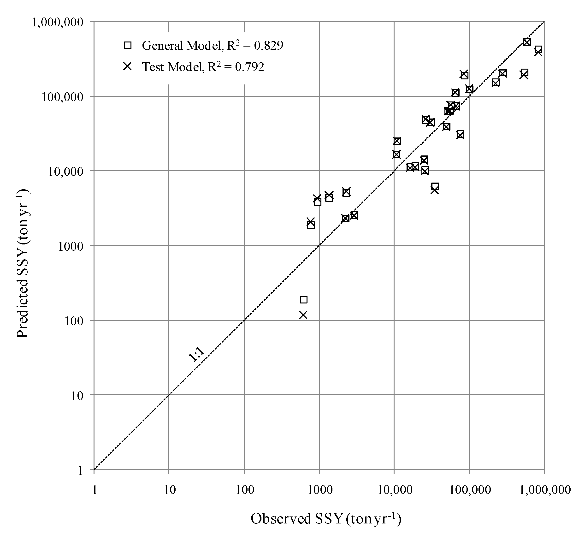
The investigation of factors affecting suspended sediment yield in the Ping, Wang, Yom and Nan river basins in Thailand, using principal component analysis, is presented in this study. From the principal component analysis, six components of dominant factors influencing suspended sediment yield were identified. These factors contribute to 86.7% of the total variance of all variables considered in the analysis. The dominant factors from each group were then taken as predictor variables in the successive multiple regression analysis to estimate suspended sediment yield and area-specific suspended sediment yield.
From the regression analysis, it was found that there are three factors that significantly affect suspended sediment yield. These factors are hierarchical anomaly density, basin area and forest area. On the other hand, there are five factors that significantly influence area-specific suspended sediment yield. These are basin slope, hierarchical anomaly density, main channel length, forest area and dry season rainfall. The regression models indicate better predictability of suspended sediment yield and area-specific sediment yield for basins with a drainage area of less than 1000 km2.
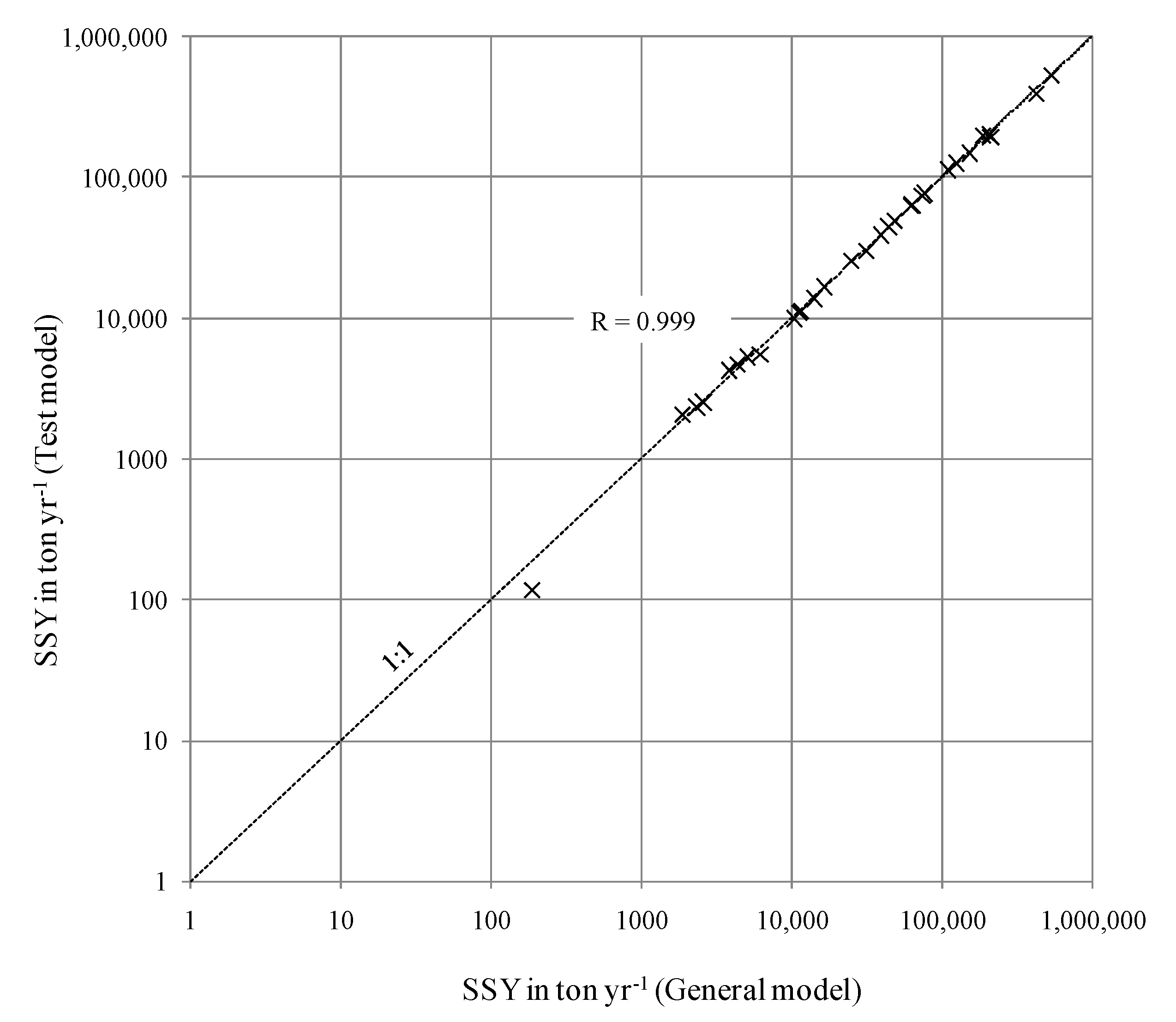
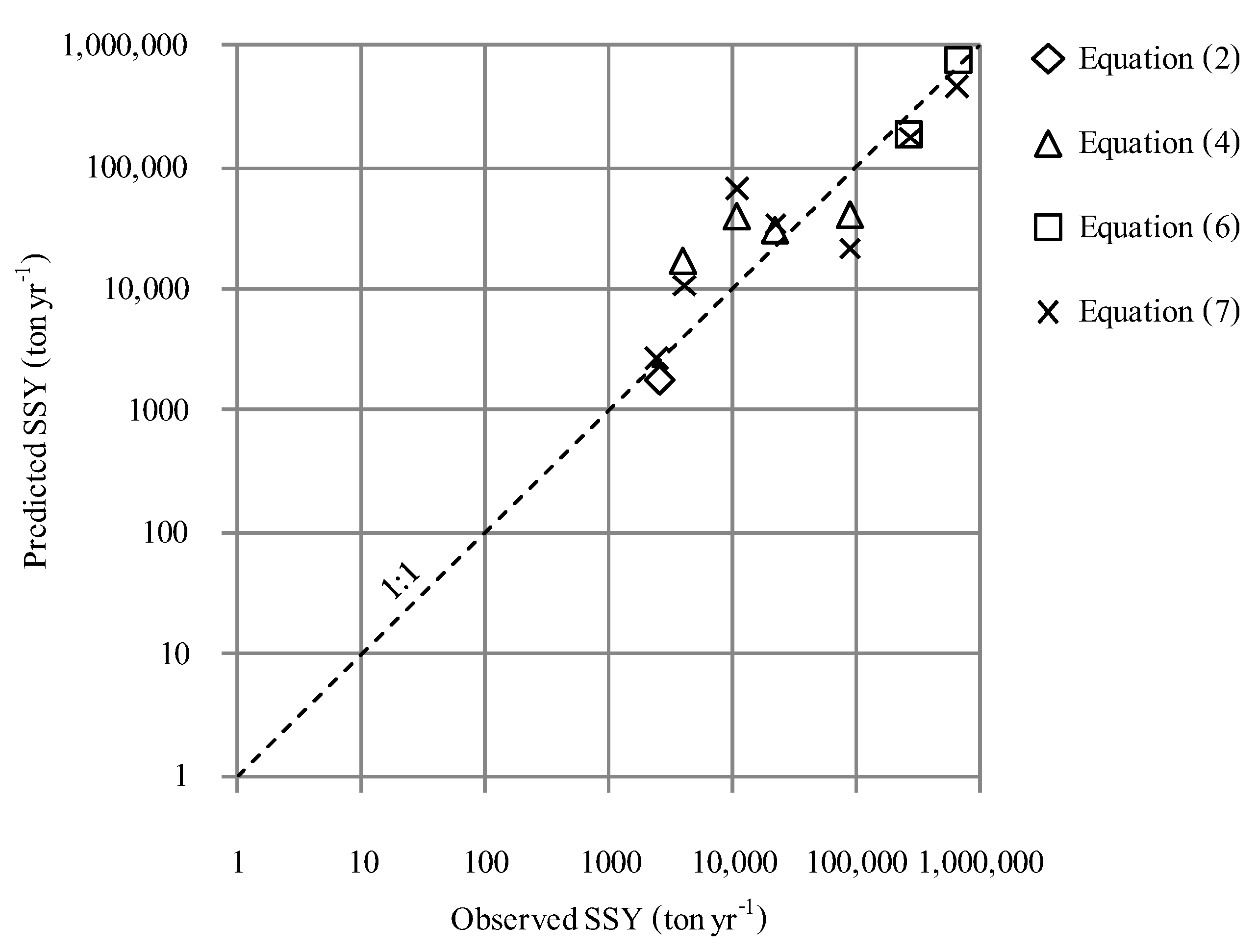
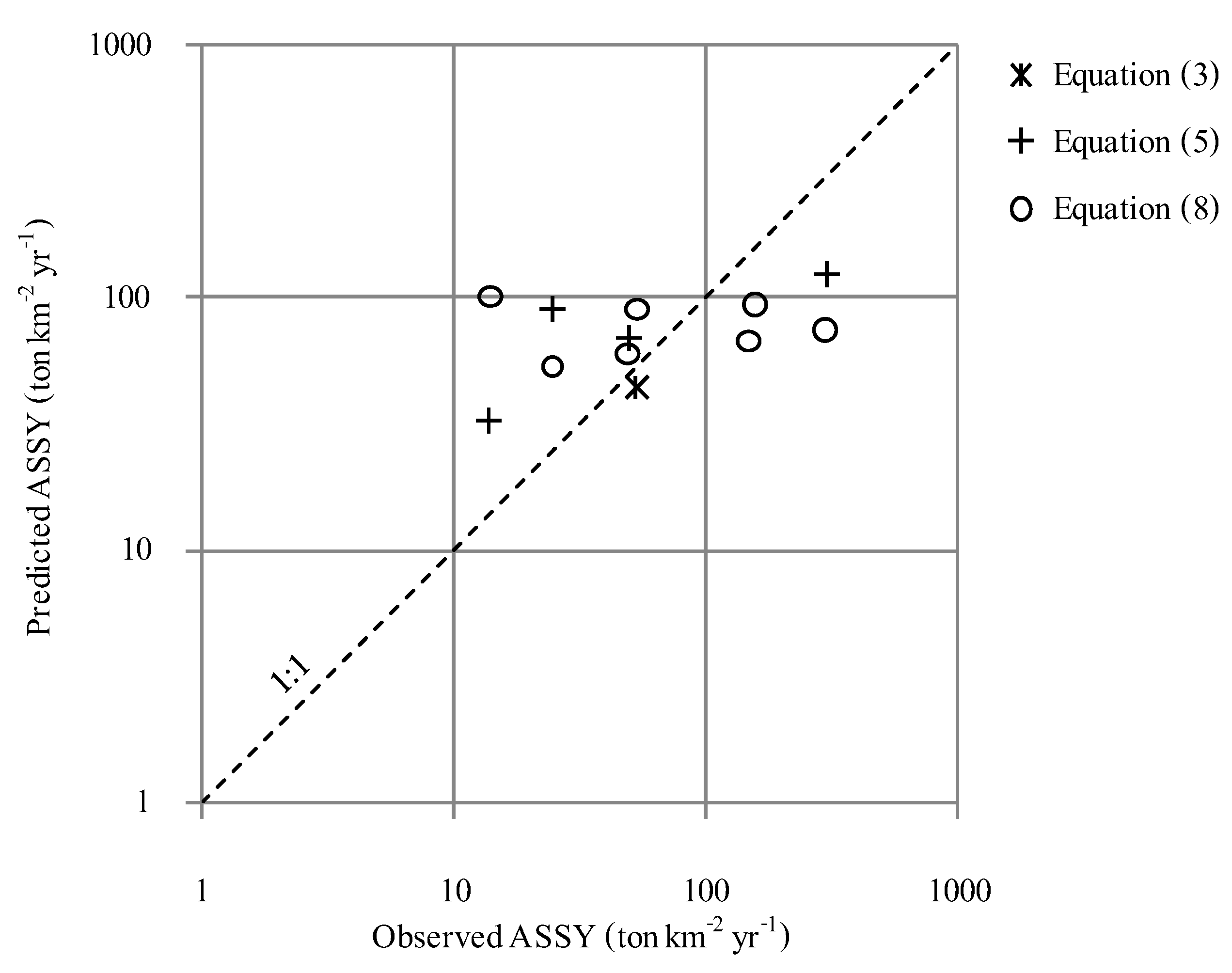
A set of equations for predicting suspended sediment yield and area-specific suspended sediment yield for basin areas with different sizes within the error of estimation range was proposed. These equations may be used to estimate the expected sediment yield in ungauged basins in the planning and design of water and land development and conservation projects in the northern part of Thailand with easily determined dominant input variables. However, it should be noted that the error of estimation for suspended sediment is relatively high, which is partially due to uncertainties in the sediment sampling/measurement (especially during high discharges or flood events) and in developing the sediment-discharge rating curve equations. Additionally, these models were developed for the estimation of average annual suspended sediment in ungauged basins. Therefore, the application of the models for sediment yield on short time periods, such as event-based estimation, is not recommended, due to the hysteresis effect in sediment rating curves.
Since this is a data-driven approach, the availability of limited data may restrain its applicability. The proposed equations may further be tested in other basins, provided that there is adequate data with similar hydrological and geo-morphological conditions. It is to be noted here that the proposed models were developed under natural conditions, without a water regulating structure; hence, the use of models in other basins with infrastructure may not be warranted. In addition, the models were developed with a relatively short period of data; hence, it is suggested that the models may be updated with a long period of data and more stations, as well as for variable climate and land use conditions. This can be done by using variable data of land use (percent of forest area and agricultural area) and the climate characteristics (annual rainfall, dry and wet season rainfall, precipitation concentration index) and, then, re-generating a new set of regression models.

Acknowledgments

This research is conducted as part of the Ph.D. studies of the first author at the Asian Institute of Technology (AIT), Thailand. It was financially supported by the Royal Thai Government and the Rajamagala’s University of Technology Lanna, North Thailand. Meteorological, hydrological and suspended sediment data were provided by the Royal Irrigation Department, the Department of Water Resources and the Thai Meteorological Department. The topography was provided by the Geo-Informatics and Space Technology Development Agency. The Land Development Department of Thailand provided the soil and land use data for the study. The authors acknowledge the support and cooperation of all of these institutions. The authors are also sincerely grateful to the anonymous reviewers for providing thorough reviews and useful suggestions.

Author Contributions

Piyawat Wuttichaikitcharoen, being the doctoral student, conducted the research, including data collection, analysis and preparation of the manuscript. Mukand Singh Babel supervised the research, discussed the results and contributed to the finalization of the manuscript.

Conflicts of Interest

The authors declare no conflict of interest.

References

  1. Grauso, S.; Fattoruso, G.; Crocetti, C.; Montanari, A. Estimating the suspended sediment yield in a river network by means of geomorphic parameters and regression relationships. Hydrol. Earth Syst. Sci. 2008, 12, 177–191. [Google Scholar]
  2. Maidment, D.R. Handbook of Hydrology; McGraw-Hill, Inc.: New York, NY, USA, 1992. [Google Scholar]
  3. Wani, S.P. Integrated Watershed Management for Sustaining Crop Productivity and Reducing Soil Erosion in Asia. In Proceedings of the 5th Management of Soil Erosion Consortium (MSEC) Assembly, Semarang, Central Java, Indonesia, 7–11 November 2001; Maglinao, A.R., Leslie, R.N., Eds.; International water Management Institute (IWMI): Semarang, Central Java, Indonesia.
  4. Shi, Z.H.; Ai, L.; Fang, N.F.; Zhu, H.D. Modeling the impacts of integrated small watershed management on soil erosion and sediment delivery: A case study in the Three Gorges area, China. J. Hydrol. 2012, 438–439, 156–167. [Google Scholar] [CrossRef]
  5. Tetzlaff, B.; Friedrich, K.; Vorderbrügge, T.; Vereecken, H.; Wendland, F. Distributed modelling of mean annual soil erosion and sediment delivery rates to surface waters. CATENA 2013, 102, 13–20. [Google Scholar] [CrossRef]
  6. Kothyari, U.C. Sediment problems and sediment management in the indian sub-himalayan region. In Sediment Problems and Sediment Management in Asian River Basins; Walling, D.E., Ed.; IAHS Press: CEH Wallingford, Oxfordshire, UK, 2011; Volume 349. [Google Scholar]
  7. Boonchee, S.; Sumalee, S.; Inthapan, P.; Rachadawong, S. Management of Sloping Lands for Sustainable Agriculture; Final Report of ASIALAND Network, Phase 4; International Water Management Institute: Bangkok, Thailand, 2002. [Google Scholar]
  8. Walling, D.E.; Webb, B.W. Erosion and sediment yield: A global overview. In Erosion and Sediment Yield: Global and Regional Perspectives; Walling, D.E., Webb, B.W., Eds.; IAHS Press: Wallingford, UK, 1996; Volume 236, pp. 3–19. [Google Scholar]
  9. White, S. Sediment yield prediction and modelling. Hydrol. Process. 2005, 19, 3053–3057. [Google Scholar] [CrossRef]
  10. Wischmeier, W.H.; Smith, D.D. Predicting Rainfall Erosion Losses—A Guide to Conservation Planning; USDA-SEA Agriculture Handbook No.537; US Department of Agriculture: Washington, DC, USA, 1978. [Google Scholar]
  11. Walling, D.E. The sediment delivery problem. J. Hydrol. 1983, 65, 113–141. [Google Scholar] [CrossRef]
  12. Maner, S.B. Factors affecting sediment delivery rates in the Red Hills physiographic area. Trans. Am. Geophys. Union 1958, 39, 669–675. [Google Scholar] [CrossRef]
  13. Williams, J.R.; Berndt, H.D. Sediment yield computed with universal equation. J. Hydraul. Div. ASCE 1972, 98, 2087–2098. [Google Scholar]
  14. Mou, J.; Meng, Q. Sediment Delivery Ratio as Used in the Computation of Watershed Sediment Yield; Chinese Society of Hydraulic Engineering: Beijing, China, 1980. [Google Scholar]
  15. Van Oost, K.; Govers, G.; Desmet, P. Evaluating the effects of landscape structure on soil erosion by water and tillage. Landsc. Ecol. 2000, 15, 579–591. [Google Scholar]
  16. Van Rompaey, A.; Krasa, J.; Dostal, T.; Govers, G. Modelling sediment supply to rivers and reservoirs in Eastern Europe during and after the collectivisation period. Hydrobiologia 2003, 494, 169–176. [Google Scholar] [CrossRef]
  17. Gurmessa, T.K.; Bárdossy, A. A principal component regression approach to simulate the bed-evolution of reservoirs. J. Hydrol. 2009, 368, 30–41. [Google Scholar] [CrossRef]
  18. Leh, M.; Bajwa, S.; Chaubey, I. Impact of land use change on erosion risk: An integrated remote sensing, geographic information system and modeling methodology. Land Degrad. Dev. 2013, 24, 409–421. [Google Scholar]
  19. Cohen, S.; Kettner, A.J.; Syvitski, J.P.M.; Fekete, B.M. WBMsed, a distributed global-scale riverine sediment flux model: Model description and validation. Comput. Geosci. 2013, 53, 80–93. [Google Scholar] [CrossRef]
  20. Balthazar, V.; Vanacker, V.; Girma, A.; Poesen, J.; Golla, S. Human impact on sediment fluxes within the Blue Nile and Atbara river basins. Geomorphology 2013, 180–181, 231–241. [Google Scholar] [CrossRef]
  21. Grauso, S.; Pagano, A.; Fattoruso, G.; Bonis, P.D.; Onori, F.; Regina, P.; Tebano, C. Relations between climatic–geomorphological parameters and sediment yield in a mediterranean semi-arid area (Sicily, Southern Italy). Environ. Geol. 2008, 54, 219–234. [Google Scholar] [CrossRef]
  22. Syvitski, J.P.M.; Milliman, J.D. Geology, geography, and humans battle for dominance over the delivery of fluvial sediment to the coastal ocean. J. Geol. 2007, 115, 1–19. [Google Scholar] [CrossRef]
  23. Restrepo, J.D.; Kjerfve, B.; Herrnelin, M.; Restrepo, J.C. Factors controlling sediment yield in a major South American drainage basin: The magdalena river, colombia. J. Geol. 2006, 316, 213–232. [Google Scholar]
  24. Liu, Q.Q.; Singh, V.P.; Xiang, H. Plot erosion model using gray relational analysis method. J. Hydrol. Eng. 2005, 10, 288–294. [Google Scholar] [CrossRef]
  25. Sharma, U.C.; Sharma, V. Mathematical model for predicting soil erosion by flowing water in ungauged watersheds. In Erosion Prediciton in Ungauged Basins: Integrating Methods and Techniques; Boer, D.D., Froehlich, W., Mizuyama, T., Pietroniro, A., Eds.; IAHS Press: Wallingford, UK, 2003; Volume 279, pp. 79–83. [Google Scholar]
  26. Hovius, N. Controls on sediment supply by large rivers, relative role of eustasy, climate, and tectonism in continental rocks. In Relative Role of Eustasy, Climate, and Tectonism in Continental Rocks; SEPM (Society for Sedimentary Geology): Tulsa, OK, USA, 1998; Volume 59, pp. 2–16. [Google Scholar]
  27. Gurnell, A.; Hannah, D.; Lawler, D. Suspended sediment yield from glacier basins. In Erosion and Sediment Yield: Global and Regional Perspectives; Walling, D.E., Webb, B.W., Eds.; IAHS Press: Wallingford, UK, 1996; Volume 236, pp. 97–104. [Google Scholar]
  28. Walling, D.E. Measuring sediment yield from river basin. In Soil Erosion Research Methods; Lal, R., Ed.; Soil and Water Conservation Society: Ankeny, IA, USA, 1994; pp. 39–80. [Google Scholar]
  29. Bray, D.I.; Xie, H. A regression method for estimating suspended sediment yields for ungauged watersheds in Atlantic Canada. Can. J. Civil Eng. 1993, 20, 82–87. [Google Scholar] [CrossRef]
  30. Ciccacci, S.; Fredi, P.; Palmieri, E.L.; Pugliese, F. Indirect evaluation of erosion entity in drainage basins through geomorphic, climatic and hydrological parameters. In International Geomorphology1986 Part II; Gardiner, V., Ed.; John Wiley & Son Ltd: Hoboken, NJ, USA, 1987. [Google Scholar]
  31. Walling, D.E.; Webb, B.W. Patterns of sediment yield. In Background to Hydrogeology; Gregory, K.J., Ed.; Wiley: Chichester, UK, 1983; pp. 69–100. [Google Scholar]
  32. Langbein, W.B.; Schumm, S.A. Yield of sediment in relation to mean annual precipitation. Trans. Am. Geophys. Union 1958, 39, 1076–1084. [Google Scholar] [CrossRef]
  33. Anderson, H.W. Relating sediment yield to watershed variables. Trans. Am. Geophys. Union 1957, 38, 921–924. [Google Scholar] [CrossRef]
  34. Brown, C.E. Use of principal-component, correlation, and stepwise multiple-regression analyses to investigate selected physical and hydraulic properties of carbonate-rock aquifers. J. Hydrol. 1993, 147, 169–195. [Google Scholar] [CrossRef]
  35. Pandzic, K.; Trninic, D. Principal component analysis of a river basin discharge and precipitation anomaly fields associated with the global circulation. J. Hydrol. 1992, 132, 343–360. [Google Scholar] [CrossRef]
  36. Hidalgo, H.G.; Piechota, T.C.; Dracup, J.A. Alternative principal components regression procedures for dendrohydrologic reconstructions. Water Resour. Res. 2000, 36, 3241–3249. [Google Scholar] [CrossRef]
  37. Bouvier, C.; Cisneros, L.; Dominguez, R.; Laborde, J.-P.; Lebel, T. Generating rainfall fields using principal components (pc) decomposition of the covariance matrix: A case study in mexico city. J. Hydrol. 2003, 278, 107–120. [Google Scholar] [CrossRef]
  38. Halim, R.; Clemente, R.S.; Routray, J.K.; Shrestha, R.P. Integration of biophysical and socio-economic factors to assess soil erosion hazard in the Upper Kaligarang watershed, Indonesia. Land Degrad. Dev. 2007, 18, 453–469. [Google Scholar] [CrossRef]
  39. Samani, N.; Gohari-Moghadam, M.; Safavi, A.A. A simple neural network model for the determination of aquifer parameters. J. Hydrol. 2007, 340, 1–11. [Google Scholar] [CrossRef]
  40. Al-Alawi, S.M.; Abdul-Wahab, S.A.; Bakheit, C.S. Combining principal component regression and artificial neural networks for more accurate predictions of ground-level ozone. Environ. Model. Softw. 2008, 23, 396–403. [Google Scholar] [CrossRef]
  41. Tayfur, G.; Karimi, Y.; Singh, V. Principle component analysis in conjuction with data driven methods for sediment load prediction. Water Resour. Manag. 2013, 27, 2541–2554. [Google Scholar]
  42. Hyvärinen, A.; Oja, E. Independent component analysis: Algorithms and applications. Neural Netw. 2000, 13, 411–430. [Google Scholar] [CrossRef]
  43. Ikeda, S.; Toyama, K. Independent component analysis for noisy data—MEG data analysis. Neural Netw. 2000, 13, 1063–1074. [Google Scholar] [CrossRef]
  44. Westra, S.; Brown, C.; Lall, U.; Koch, I.; Sharma, A. Interpreting variability in global SST data using independent component analysis and principal component analysis. Int. J. Climatol. 2010, 30, 333–346. [Google Scholar]
  45. 25 River Basins Report; Royal Irrigation Department, Ministry of Agriculture and Cooperatives: Bangkok, Thailand, 2003. (In Thai)
  46. Alford, D. Streamflow and sediment transport from mountain watersheds of the Chaophraya basin, Northern Thailand: A reconnaissance study. Mt. Res. Dev. 1992, 12, 257–268. [Google Scholar] [CrossRef]
  47. Tingting, L.V.; Xiaoyu, S.; Dandan, Z.; Zhenshan, X.; Jianming, G. Assessment of Soil Erosion Risk in Northern Thailand; Jun, C., Ed.; International Archives of the Photogrammetry, Remote Sensing and Spatial Information Sciences: Beijing, China, 2008. [Google Scholar]
  48. Plangoen, P.; Babel, M.; Clemente, R.; Shrestha, S.; Tripathi, N. Simulating the impact of future land use and climate change on soil erosion and deposition in the Mae Nam Nan sub-catchment, Thailand. Sustainability 2013, 5, 3244–3274. [Google Scholar] [CrossRef]
  49. Wigmosta, M.S.; Vail, L.W.; Lettenmaier, D.P. A distributed hydrology-vegetation model for complex terrain. Water Resour. Res. 1994, 30, 1665–1679. [Google Scholar] [CrossRef]
  50. HEC-GeoHMS Geospatial Hydrologic Modeling Extension User’s Manual Version 10.1; US Army Corps of Engineers, Hydrologic Engineering Center: Davis, CA, USA, 2013.
  51. Department of Water Resources. Standard Map of Main and Sub-River Basins Delineation of Thailand; Sahamitr Printing & Publishing Co., Ltd: Nonthaburi, Thailand, 2009. (In Thai) [Google Scholar]
  52. Guarnieri, P.; Pirrotta, C. The response of drainage basins to the late quaternary tectonics in the Sicilian side of the Messina Strait (NE Sicily). Geomorphology 2008, 95, 260–273. [Google Scholar] [CrossRef]
  53. Della Seta, M.; del Monte, M.; Fredi, P.; Palmieri, E.L. Direct and indirect evaluation of denudation rates in Central Italy. CATENA 2007, 71, 21–30. [Google Scholar] [CrossRef]
  54. Carter, A.J.; Scholes, R.J. Generating a Global Database of Soil Properties; Council for Scientific and Industrial Research (CSIR) Environmentek: Pretoria, South Africa, 1999. [Google Scholar]
  55. Batjes, N.H. A Homogenized Soil Data File for Global Environmental Research: A Subset of FAO, ISRIC and NRCS Profiles (Version 1.0); Working paper and preprint 95/10b; International Soil Reference and Information Centre: Wageningen, The Netherlands, 1995. [Google Scholar]
  56. Digital Soil Map of the World, Version 3.5, Food and Agriculture Organization of the United Nations: Rome, Italy, 1995.
  57. Royal Irrigation Department. Monthly and Annual Suspended Sediment in Main River Basins of Thailand; Sediment and Water Quality Group, Hydrology Division, Royal Irrigation Department: Bangkok, Thailand, 2011. (In Thai) [Google Scholar]
  58. De Luís, M.; Raventós, J.; González-Hidalgo, J.C.; Sánchez, J.R.; Cortina, J. Spatial analysis of rainfall trends in the region of Valencia (East Spain). Int. J. Climatol. 2000, 20, 1451–1469. [Google Scholar] [CrossRef]
  59. Petras, I. Arcview Arealrain Extension; Department of Water Affairs and Forestry: Pertoria, South Africa, 2001. [Google Scholar]
  60. Landau, S.; Everitt, B.S. A Handbook of Statistical Analyses Using SPSS; CRC Press Company: London, UK, 2003. [Google Scholar]
  61. Pallant, J. SPSS Survival Manual: A Step by Step Guide to Data Analysis Using SPSS; Allen & Unwin: Crows Nest, NSW, Australia, 2005. [Google Scholar]
  62. Haan, C.T. Statistical Methods in Hydrology, 2nd ed.; The Iowa State Press: Ames, IA, USA, 2002; p. 496. [Google Scholar]
  63. Kaiser, H. An index of factorial simplicity. Psychometrika 1974, 39, 31–36. [Google Scholar] [CrossRef]
  64. Bartlett, M.S. A note on the multiplying factors for various chi square approximations. J. R. Stat. Soc. 1954, 16, 296–298. [Google Scholar]
  65. Hair, J.F.; Black, B.; Babin, B.; Anderson, R.E.; Tatham, R.L. Multivariate Data Analysis, 6th ed.; Pearson Printice Hall: Upper Saddle River, NJ, USA, 2006. [Google Scholar]
  66. Tabachnick, B.G.; Fidell, L.S. Using Multivariate Statistics; Harper Collins: New York, NY, USA, 2001. [Google Scholar]
  67. Brejda, J.J.; Moorman, T.B.; Karlen, D.L.; Dao, T.H. Identification of regional soil quality factors and indicators: I. Central and southern high plains. Soil Sci. Soc. Am. J. 2000, 64, 2115–2124. [Google Scholar] [CrossRef]
  68. Andrews, S.S.; Mitchell, J.P.; Mancinelli, R.; Karlen, D.L.; Hartz, T.K.; Horwath, W.R.; Pettygrove, G.S.; Scow, K.M.; Munk, D.S. On-farm assessment of soil quality in california’s central valley. Agron. J. 2002, 94, 12–23. [Google Scholar] [CrossRef]
  69. National Engineering Handbook, Section 3: Sedimentation, 2nd ed.; United States Department of Agriculture, Soil Conservation Service: Washington, DC, USA, 1983.
  70. Noble, R.; Cowx, I. Development of a River-Type Classification System (D1), Compilation and Harmonisation of Fish Species Classification (D2); Final Report of Development, Evaluation & Implementation of a Standardised Fish-Based Assessment Method for the Ecological Status of European Rivers—A Contribution to the Water Framework Directive (FAME). FAME Group, University of Hull: Hull, UK, 2002; p. 51. Available online: https://fame.boku.ac.at/downloads/ D1_2_typology_and%20species_classification.pdf (accessed on 10 August 2013).
  71. Stevens, J. Applied Multivariate Statistics for the Social Sciences; Lawrence Erlbaum: Mahwah, NJ, USA, 1996. [Google Scholar]
  72. Kazama, S.; Suzuki, K.; Sawamoto, M. Estimation of rating-curve parameters for sedimentation using a physical model. Hydrol. Process. 2005, 19, 3863–3871. [Google Scholar] [CrossRef]

