1. Introduction
According to [
1], floods are among the most recurring and devastating natural hazards, impacting upon human lives and causing severe economic damage throughout the world. It is understood that flood risks will not subside in the future, and with the onset of climate change, flood intensity and frequency will threaten many regions of the world [
2].
Floods occur because of the rapid accumulation and release of runoff waters from upstream to downstream, which is caused by very heavy rainfall. Discharges quickly reach a maximum and diminish almost as rapidly. The occurrence of flooding is of concern in hydrologic and natural hazards science due to the top ranking of such events among natural disasters in terms of both the number of people affected globally and the proportion of individual fatalities [
3]. The potential for flood casualties and damages is also increasing in many regions due to the social and economic development, which imply pressure on land-use, e.g., through urbanization. Flood hazard is expected to increase in frequency and severity, through the impacts of global change on climate, severe weather in the form of heavy rains and river discharge conditions [
4]. The current trend and future scenarios of flood risks therefore demand for accurate spatial and temporal information on the potential hazards and risks of floods.
As reported by [
5], heavy convective rainfall often results in flooding in urban areas. Urbanization results into conversion of agricultural land, natural vegetation and wetlands to built-up environments and construction on natural drainages as well increase in the population of those living in flood vulnerable areas such as flood plains and river beds. According to [
6], there is a direct relationship between urbanization and hydrological characteristics; decreased infiltration, increase in runoff, increase in frequency and flood height. In addition to population growth and the ongoing accumulation of value assets, both the frequency and magnitude of floods due to climate change are expected to increase in the future, therefore aggravating the existing flood risk in urban areas. This scenario implies that urban areas in particular suffer from a comparatively high flood risk due to their high population number and density, multiple economic activities and many infrastructure and property values, that in turn interferes with the natural infiltration processes.
The high risk potential of floods in particular may be related to their rapid occurrence and to the spatial dispersion of the areas which may be impacted by these floods. Both characteristics limit the ability to issue timely flood warnings. In flood prone areas, runoff rates often far exceed those of other water flow types due to the rapid response of the catchments to intense rainfall, modulated by soil moisture and soil hydraulic properties. The small spatial and temporal scales of floods, relative to the sampling characteristics of conventional rain and discharge measurement networks, make also these events particularly difficult to observe and to predict [
3].
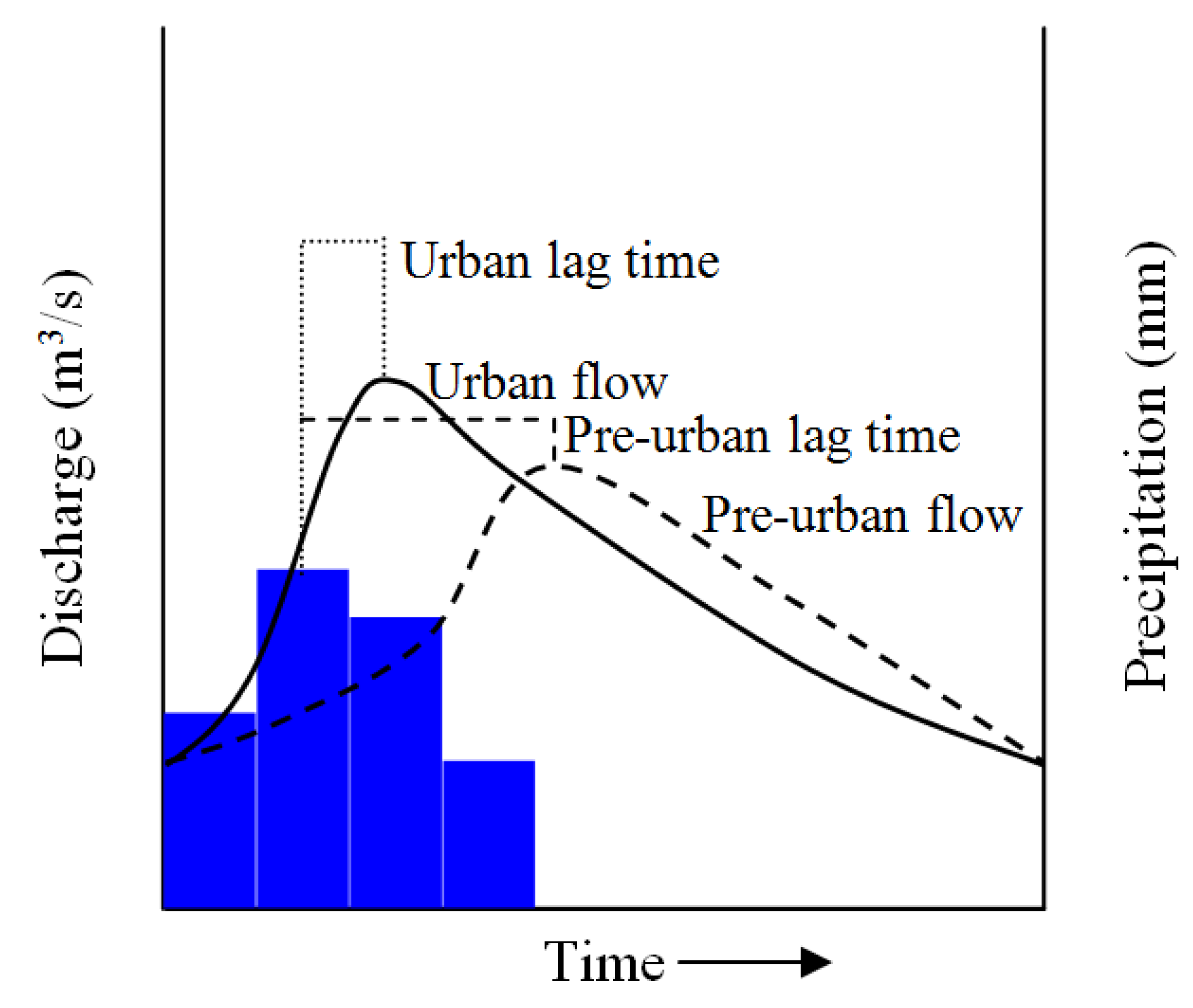
Small streams in urban areas can also rise quickly after heavy rain due to higher generated runoff and less concentration time as depicted in
Figure 1 [
7]. Changes in the urban area and in storm intensity produce higher flows that exceed the capacity of small culverts under roads designed for non-urbanized areas. Although such structures can be adequate when designed, their capacity may turn out to be inadequate and thereby cause overflows onto the roads creating new water paths and flood the built up areas. In developing countries, inadequate maintenance of the drainage channels, and debris and solid waste disposed into such drainage systems may accentuate the situation [
8]. The rainfall runoff process, however, is highly complex, non-linear and temporally and spatially varying because of the variability of the terrain and climate attributes [
5].
Figure 1.
Typical Hydrograph of urban and non-urban area.
Figure 1.
Typical Hydrograph of urban and non-urban area.
Flood risk maps need therefore to be created as they provide a basis for the development of flood risk management plans. What is more, these plans need to be effectively communicated to various target groups (including decision makers, emergency response units and the public) as a measure to reduce flood risk by integrating different interests, potential and conflicts over space and land use in a city.
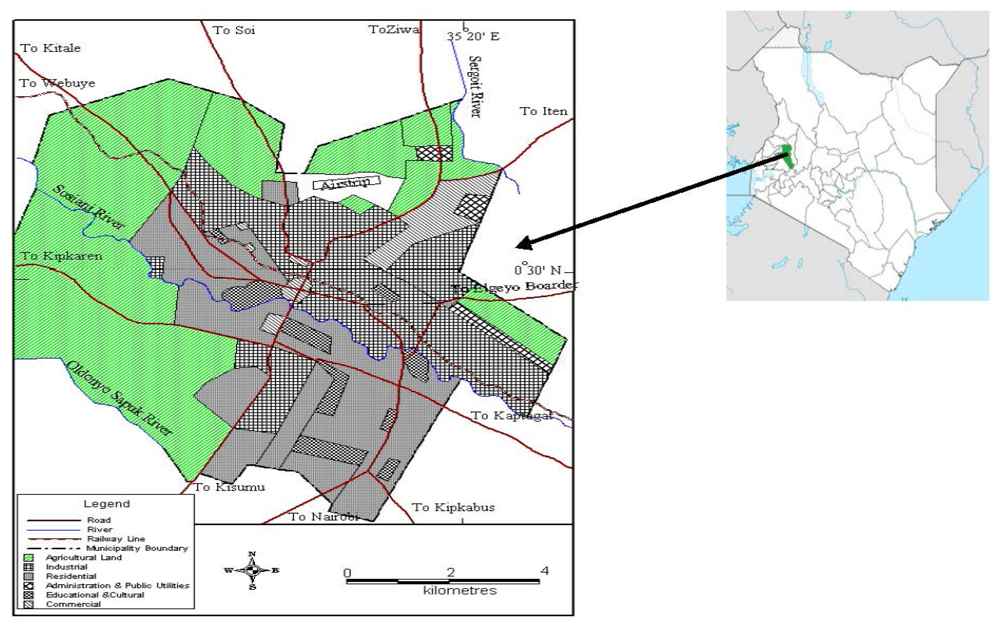
Urban flood risk vulnerability assessment thus requires detailed knowledge about the risk in respective parts of a town or municipality to be effective and of use for urban planning and hazard management. In this context, the following research questions are addressed: (i) which criteria of risk should be considered for an urban integrated flood risk assessment and (ii) how do differently weighted criteria sets alter both the value and spatial distribution of the multi-criteria flood risk in an urban area. The present study presents an integrated approach using Geographical Information System (GIS) and Analytic Hierarchy Process (AHP) for creating flood hazard map from the available data base, for the case study of Eldoret Municipality in Kenya.
The objectives of the current study are: (i) to develop a hierarchical structure through the analytic hierarchy process to provide preferred options for flood risk analysis; (ii) to map the relative flood risk using AHP in a GIS environment GIS; (iii) to integrate these two methodologies and apply them to an urban case study; and (iv) carry out an urban flood risk index (UFRI) mapping for the case study.
The rest of the paper is organized as follows:
Section 2 is focused on the case study area description and the flooding problem in the study area of Eldoret Municipality.
Section 3 and
Section 4 expounds on the concept, motivation and the implementation of multi-criteria decision making (MCDM) using multi-parametric approach for urban flood risk mapping using the proposed AHP-GIS approach.
Section 5 presents the descriptions and analysis of the used data sources in this case study. The results are discussed in
Section 6, presented before coming to some conclusions in
Section 7.
3. Spatial Information and Multi-Criteria Evaluation for Flood Vulnerability Mapping
Flooding risk consists of hazard and vulnerability. Hazards can be defined as threatening events, or the probability of occurrence of a potentially damaging phenomena within a given time period and area. When a hazardous event occurs, the damage depends on the elements at risk. The elements at risk are the population, buildings and civil engineering structures, economic activities, public services and infrastructure [
10].
Vulnerability on the other hand is the most crucial component of risk in that it determines whether or not exposure to a hazard constitutes a risk that may actually result in a disaster. If the potential exposure to floods becomes a reality,
i.e., when floodwaters physically encroach on a populated area or infrastructure, then the vulnerability of people and infrastructure is decisive for the degree of harm and damage. The physical vulnerability of urban populations tends to increase because of the dense concentration of potentially dangerous infrastructure and substances in urban areas. Additionally, the existence of health threatening infrastructure such as sewage treatment plants or dangerous industries at such locations increases the risk of secondary hazards and damage. This type of risk can be categorized in urban or non-urban depending on the localization of the flooding event. Special attention in the context of human settlement locations must therefore be paid to socio-economic factors [
7]. The integration of flood risk in territorial management, e.g., urban or municipal areas needs a better knowledge of the associated vulnerabilities.
To provide flood risk assessment information on the probability of flood occurrence, magnitude of the event, location and depth of the inundation for flood management, most studies have applied hydrologic and hydraulic models to simulate flood runoff and runoff in low-lying and flood-prone areas [
11]. The authors of [
12] assessed the flood risks using hydraulic models coupled with the GIS and Digital Elevation Model (DEM) to map the area and depth of inundation. [
13] presented the technique for preparation of flood hazard maps which include development of digital elevation model and simulation of flood flows of different return periods. In [
14], the authors proved that GIS technique is effective in extracting the flood inundation extent in a time and cost-effective manner for the remotely located hilly basin of Dikrong, where conducting conventional surveys is very difficult. Further, [
15] used GIS to demarcate the flood hazard prone areas in the Papanasam Taluk into five zones of varying degrees of flooding. Moreover, [
16] stated that a flood risk map should be able to identify the areas that are most vulnerable to flooding and estimate the number of people that will be affected by floods in a particular area.
All disasters have a spatial component and therefore adequate geographic information on hazards and areas vulnerable to hazards is required in order to be able to prepare for disasters. Multi-criteria evaluation (MCE) methods have been applied in several studies since 80% of data used by decision makers is related to geography [
17]. GIS may provide more and better information about decision making situations as it allows the decision maker to identify and list a predefined set of criteria with the overlay process. Multi-criteria decision analysis within GIS may be used to develop and evaluate alternative plans that may facilitate compromise among interested parties [
17].
The main advantage of using GIS for flood analyses is that it not only generates a visualization of flooding, but also creates potential to further analyze these events to estimate probable damage due to floods. Compared to traditional mapping, GIS enables the comparisons across spatial units; comparison across different themes by category of hazards and disasters; merging of qualitative with qualitative assessment and spatial database, based on which logical and/or numerical operations can be dynamically performed. These are grounds for concluding that GIS has an important function to play in natural hazards analyses because natural hazards are multi-dimensional phenomena, which have a spatial component [
18].
Most conventional GIS based methods for flood risk mapping [
19] are based on ground surveys and aerial observations, but when the phenomenon is widespread, such methods are time consuming and expensive. Furthermore, timely aerial observations may be impossible due to prohibitive weather conditions. This study therefore proposes a multi-parametric approach for delineating flood vulnerability in a growing urban area through the integration of Analytical Hierarchical Process (AHP) as a multi-criteria decision making (MCDM) technique within a GIS mapping environment. The effectiveness of AHP in evaluating problems involving multiple and diverse criteria and the measurement of trade-offs—sometimes using limited available data—has led to its recognition across different fields of application [
20].
The multi-criteria analysis methods provide a framework which can handle different views on the identification of the elements of a complex decision problem, organize the elements into a hierarchical structure, and study the relationships among components of the problem [
21]. The use of this method in the context of flood risk management is still rare [
22].
AHP as an MCA approach has been used for solving various flooding problems. In [
23], the authors used AHP to select the optimal flood control projects for the Grand River and Tar Creek in Miami, USA. In India, flood risk analysis using AHP and mapped by GIS has been applied to the Kosi River Basin [
24]. The authors of [
25] employed a two-dimensional diffusive overland flow model to simulate inundation status in northern Taiwan, and further used GIS to illustrate the area and depth of inundation. Based on the inundation map, they developed a model to evaluate the possible damage from floods by using grey AHP. AHP was also used to rank the importance of loss of life and different properties, which is the flood index [
24,
25]. The total ranks of the index of possible damage were then mapped by using GIS [
26]. The above reviews shows that AHP is mostly applied in natural environments and not in developed urban areas.
Floods place the problem of un-gauged area prediction under rather extreme conditions. Process understanding is required for flood risk management, because the dominant processes of runoff generation may change with the increase of storm severity, and therefore, the understanding based on analysis of moderate floods may be questioned when used for forecasting the response to extreme storms. This means that flood mapping in most developing countries, which are mostly un-gauged, is a complex problem that should integrate data scarcity and uncertainty in the analysis and decision-making process. Notable is the fact that most studies have concentrated on flood mitigation and management [
2], but less has been done on pre-flood mapping.
With the AHP-GIS approach, the aim of this study is to create an easily-readable flood vulnerability map based on morphometric and topographic data. Through a multi-parametric analysis, a composite index map is computed for the urban flood hazard mapping. By weighting the flood causative criteria within the urban area, an urban flood risk index (UFRI) is derived, in combination with the vulnerability map.
4. AHP as a Multi-Criteria Decision Analysis Tool
As with all decision making processes, the expert usually engages the decision maker(s) to appropriately structure the problem. AHP has the advantage of permitting a hierarchical structure of the criteria, which provides users with a better focus on specific criteria and sub-criteria when allocating the weights. This approach is important, because a different structure may lead to a different final ranking. Criteria with a large number of sub-criteria tend to receive more weight than when they are less detailed.
In the application of multi-criteria decision analysis, the analytic hierarchy process, which is a structured technique for dealing with complex decisions, was applied in structuring the flood causative factors. Theoretically, the AHP rather than prescribing a correct decision, aids decision makers find the one that best suits their needs and their understanding of the problem. This implies that AHP is a decision making approach based on the genuine ability of people to make critical decisions. It allows the active participation of decision makers in exploring all possible options in order to fully understand the underlying problems before reaching an agreement or arriving at a decision [
27]. Therefore, the purpose of AHP is to judge the given alternatives for a particular goal by developing priorities for these alternatives and for the selected criteria.
In the AHP implementation, a pairwise comparison technique is used to derive the priorities for the criteria in terms of their importance in achieving the goal. Similarly, the priorities for the alternatives (
i.e., the competing choices under consideration) are derived in pairwise comparisons in terms of their performance against each criterion. AHP is thus based on three principles: decomposition, comparative judgment, and synthesis of priorities [
28].
By organizing and assessing alternatives with regards to a hierarchy of multifaceted attributes as depicted in
Figure 4, AHP provides an effective quantitative decision making tool to deal with complex and unstructured problems. AHP allows a better, easier, and more efficient framework for the identification of selection criteria, calculating their weights and analysis [
29]. The process therefore makes it possible to incorporate judgments on intangible qualitative criteria alongside tangible quantitative criteria.
Once the hierarchy has been constructed, the expert(s) and participants use AHP to establish priorities for all its nodes. By doing so, information is elicited from the experts and participants, and processed mathematically. Priorities are distributed over a hierarchy according to its architecture, and their values depend on the information entered by users of the process as illustrated in
Table 1. In AHP, multiple pairwise comparisons are based on a standardized comparison scale of nine levels (
Table 1). The nine points are chosen because psychologists conclude that, nine objects are the most that an individual can simultaneously compare and consistently rank. Pairwise judgements are made based on the best information available and the decision maker’s knowledge and experience.
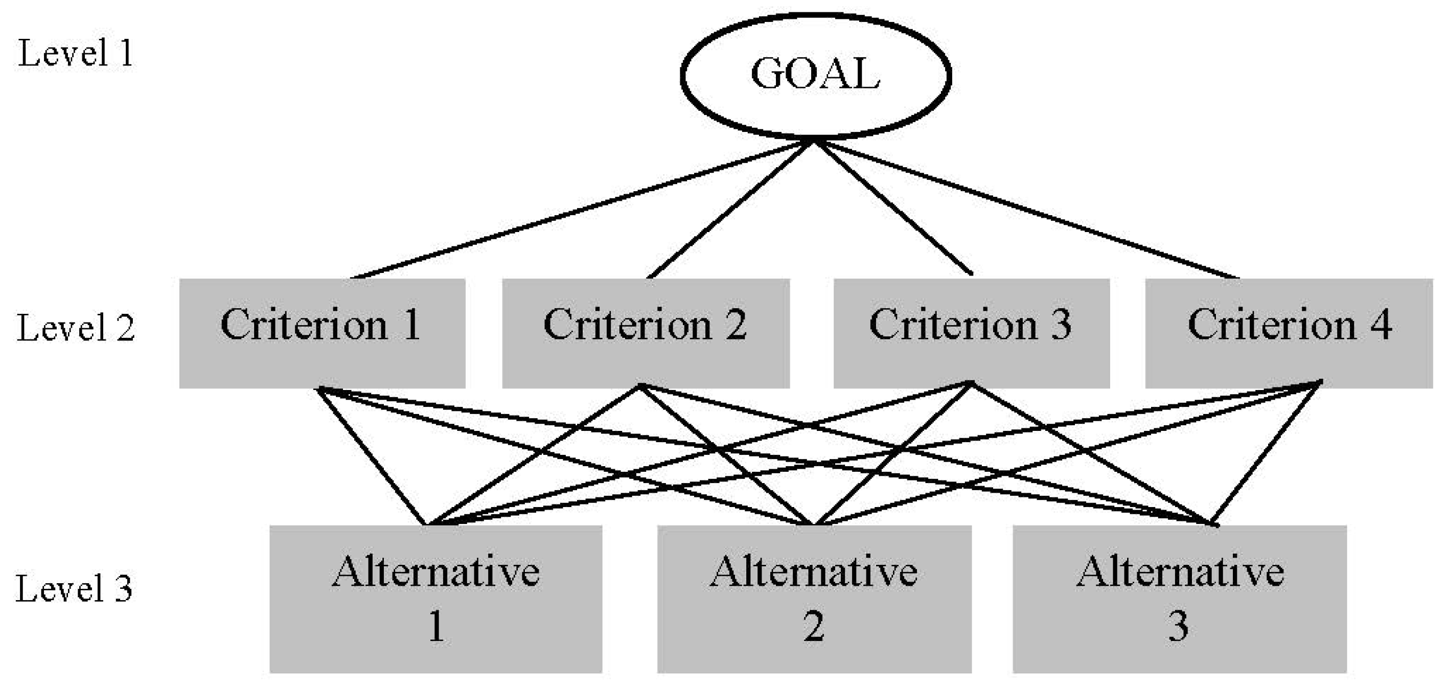
Figure 4.
The general structure of analytical hierarchy process (AHP) for multi-criteria decision making, modified from Zahedi [
30]. Copyright 1986 INFORMS PubsOnline. The goal is to choose among the competing alternatives 1, 2, and 3 on the basis of a ranking score when judged individually against criteria 1, 2, 3, and 4.
Table 1.
Nine-point intensity of importance scale, modified from Schoenherr [
31], Copyright 2008 Elsevier.
Table 1.
Nine-point intensity of importance scale, modified from Schoenherr [31], Copyright 2008 Elsevier.
| Intensity of importance | Definition | Description |
|---|
| 1 | Equally important | Two factors contribute equally to the objective. |
| 3 | Moderately more important | Experience and judgment slightly favor one over the other. |
| 5 | Strongly more important | Experience and judgment strongly favor one over the other. |
| 7 | Very strong more important | Experience and judgment very strongly favor one over the other. Its importance is demonstrated in practice. |
| 9 | Extremely more important | The evidence favoring one over the other is of the highest possible validity. |
| 2, 4, 6, 8 | Intermediate values | When compromise is needed. |
| Reciprocals of above | If an element
i has one of the above numbers assigned to it when compared with element j, then j has the reciprocal value when compared with i | – |
| Ratios (1.1–1.9) | If the activities (elements) are very close | May be difficult to assign the best value, but when compared with other contrasting activities (elements) the size of the small numbers would not be too noticeable, yet they can still indicate the relative importance of the activities (elements). |
The process of AHP can be summarized in four steps: construct the decision hierarchy; determine the relative importance of attributes and sub-attributes; evaluate each alternative and calculate its overall weight in regard to each attribute, and check the consistency of the subjective evaluations [
31]. In the first step, the decision is decomposed into its independent elements and represented in a hierarchy diagram, which should have at least three levels (goal, attributes, and alternatives) (
Figure 4). Second, the user is asked to subjectively evaluate pairs of attributes on a nine-point scale. In the third stage, a weight is calculated for each attribute (and sub-attribute), based on the pairwise comparisons. Because judgments are given subjectively by the user, the logical consistency of these evaluations is tested in the last stage. The ultimate outcome of the AHP is a relative score for each decision alternative, which can be used in the subsequent decision making process.
AHP has been successfully used in different fields and disciplines as summarized in [
32]. The ability to handle both qualitative as well as quantitative data makes AHP an ideal methodology for some prioritization problems by considering different criteria. This is mathematically outlined below.
Let
C = {
Cj |
j = 1,2,…..,
n} be the set of criteria. The result of the pairwise comparison on
n criteria can be summarized in an (
n_
n) evaluation matrix
A in which every element
aij (
i, j = 1,2,…..,
n) is the quotient of weights of the criteria, as given in Equation (1).
At the last step of AHP, the mathematical process commences to normalize and find the relative weights for each matrix. The relative weights are given by the right eigenvector (
w) corresponding to the largest eigenvalue (λ
max) as in Equation (2).
If the pairwise comparisons are completely consistent, the matrix
A has rank 1 and λ
max =
n. In this case, weights can be obtained by normalizing any of the rows or columns of
A [
33]. It should be noted that the quality of the output of the AHP is strictly related to the consistency of the pairwise comparison judgments. The consistency is defined by the relation between the entries of
A:
aij ×
ajk =
aik. The consistency index
CI is given by Equation (3):
The final consistency ratio (
CR), usage of which lets the user to conclude whether the evaluations are sufficiently consistent, is calculated as the ratio of the
CI and the random index (
RI), as expressed in Equation (4). The values of
RI are tabulated in
Table 2.
The maximum threshold of the
CR is 10%, and in case of exceedance a three-step procedure is followed [
28]: (i) identify the most inconsistent judgment in the decision matrix; (ii) determine a range of values the inconsistent judgment can be changed to so that would reduce the associated inconsistency; and (iii) ask the decision maker to reconsider the judgment to a “reasonable value”.
Table 2.
Random index (RI) used to compute consistency ratios (CR).
Table 2.
Random index (RI) used to compute consistency ratios (CR).
| N | 1 | 2 | 3 | 4 | 5 | 6 | 7 | 8 | 9 | 10 |
|---|
| Random Index (RI) | 0 | 0 | 0.58 | 0.90 | 1.12 | 1.24 | 1.32 | 1.41 | 1.45 | 1.49 |
The random index in
Table 2 is obtained by averaging the
CI of a randomly generated reciprocal matrix [
28]. The measurement of consistency can be used to evaluate the consistency of decision makers as well as the consistency of overall hierarchy [
33].
The above AHP steps can be summarized into five fundamental steps as follows [
34].
Step 1: Modeling the problem
The very first step includes stating the problem, broadening the objectives of the problem by considering all actors, objectives and corresponding outcomes, and the identification of decision elements such as alternatives and criteria or decision rules. The decision elements are set up into a hierarchy of interrelated decision elements constituting the goal, criteria, sub-criteria, and alternatives [
35]. This step has been thought to be the most important aspect of AHP [
30]. At the topmost position of the hierarchy is the overall goal (
i.e., level 1), such as the goal of selecting the best alternative. The next lower level (
i.e., level 2) of the hierarchy includes the decision rules or criteria that contribute to the attainment of the overall goal. This level can be expanded depending on how much detail is considered for each decision rule or criterion. The lowest level (
i.e., level 3) contains the alternative decisions from which the decision analyst/maker will select. A simplified general structure of the AHP is presented in
Figure 4.
Step 2: Determining Priorities among the Decision Elements of the Hierarchy
This step involves the gathering of ratings for each of the criteria and alternatives using a pairwise comparison technique and the rating scale of relative importance. This step invokes the participation of experts and/or stakeholders in determining the relative importance of one criterion or alternative over another through a pairwise comparison method presented in a matrix [
28]. The number of comparisons for the decision elements (
i.e., criteria or alternatives) in a particular level is derived using (Number of comparisons = n (n – 1)/2) [
36]. Each comparison (e.g., Criteria 1
versus Criteria 2 or Alternative 1
versus Alternative 2) is rated by a group of experts using the scale developed by [
28] for a pairwise comparison technique (
Table 1). To incorporate a group consensus, the process generally includes a questionnaire for comparing all elements and a geometric mean to arrive at a final solution [
35].
Step 3: Deriving the Overall Relative Weights of the Decision Elements
In this step, the relative importance of the criteria, as far as the attainment of the goal is concerned, and the relative importance of the alternatives with respect to the criteria are determined after a pairwise comparison matrix for the criteria and for the alternatives have been prepared (Step 2). This is done by: (i) calculating the normalized values for each criterion and alternative; and (ii) determining the normalized principal eigenvectors or priority vectors (herein also referred to as relative weights). In calculating the normalized values for each criterion and alternative in their respective matrices, the value for each cell is divided by its column total. This process produces a column total of 1 for each criterion and alternative. The relative weights are then calculated by averaging the rows of each matrix. The resulting values give the relative weights of the criteria with respect to the goal, and the relative weights of the alternatives with respect to the criteria. The overall relative weights of the alternatives are determined by calculating the linear combination (LC) of the product between the relative weight of each criterion and the relative weight of the alternative for that criterion [
36]. If the expert judgments are consistent (see Steps 4 and 5), the decision makers then select the best choice based on the overall relative weights of the alternatives.
Steps 4 and 5: Verifying the Consistency of Judgments and Making Conclusions Based on the Results
These steps are necessary to determine the consistency of the evaluation by calculating the consistency ratio before a decision is made. If the problem under consideration was aimed at selecting the best alternative, the CRs for all the matrices (
i.e., for the criteria and the alternatives) are calculated first before the overall relative weights of the alternatives are computed. Perform calculations to find the maximum eigenvalue, consistency index, consistency ratio, and normalized values for each criteria/alternative. In [
37] it is suggested that if the ratio exceeds 0.1, the set of judgments may be too inconsistent to be reliable. Thus, a CR below 0.1% or 10% is acceptable. When the evaluation is inconsistent, the procedure is repeated until the CR is within the desired range. Decision makers then reach a conclusion based on the results.
4.1. Development of AHP Decision Hierarchical Structures
Decision hierarchical structure includes the decomposition of the complex decision problem into smaller manageable elements of different hierarchical levels/layers. A four-level hierarchical tree is illustrated in
Figure 5. The first layer of the hierarchy corresponds to objective or goal, and the last layer corresponds to the evaluation alternatives (options), whereas the intermediate levels correspond to criteria and sub-criteria, depending on the project. The structure presented in
Figure 5 is derived from the generalized concept presented in
Figure 4.
Figure 5.
Decision hierarchical structure for a four-level problem decomposition, modified from Sadiq
et al. [
38]. Copyright 2004 IWA Publishing. The levels can be reduced to 3 or more than 4 depending on the complexity of the criterion elements.
Figure 5.
Decision hierarchical structure for a four-level problem decomposition, modified from Sadiq
et al. [
38]. Copyright 2004 IWA Publishing. The levels can be reduced to 3 or more than 4 depending on the complexity of the criterion elements.
In
Figure 5, the nomenclature adopted for each item in the hierarchical model is
![Water 06 01515 i004]()
, where
i is the order of the child at the level/layer
k, and
j is the parent of the child [
38]. For example,
![Water 06 01515 i005]()
represents the item is at level
k = 2, is the first child
i = 1 and its parent is
j = 1. Each child, in the intermediate levels, is criterion and sub-criterion that affect the corresponding parent and child, respectively. The apostrophe on any intermediate item (element, factor, sub-criterion),
![Water 06 01515 i006]()
, indicates that the element does not have dependent children. The ensuing derivation and discussions are limited to the shaded items located at levels 2 and 3 (
i.e.,
![Water 06 01515 i007]()
).
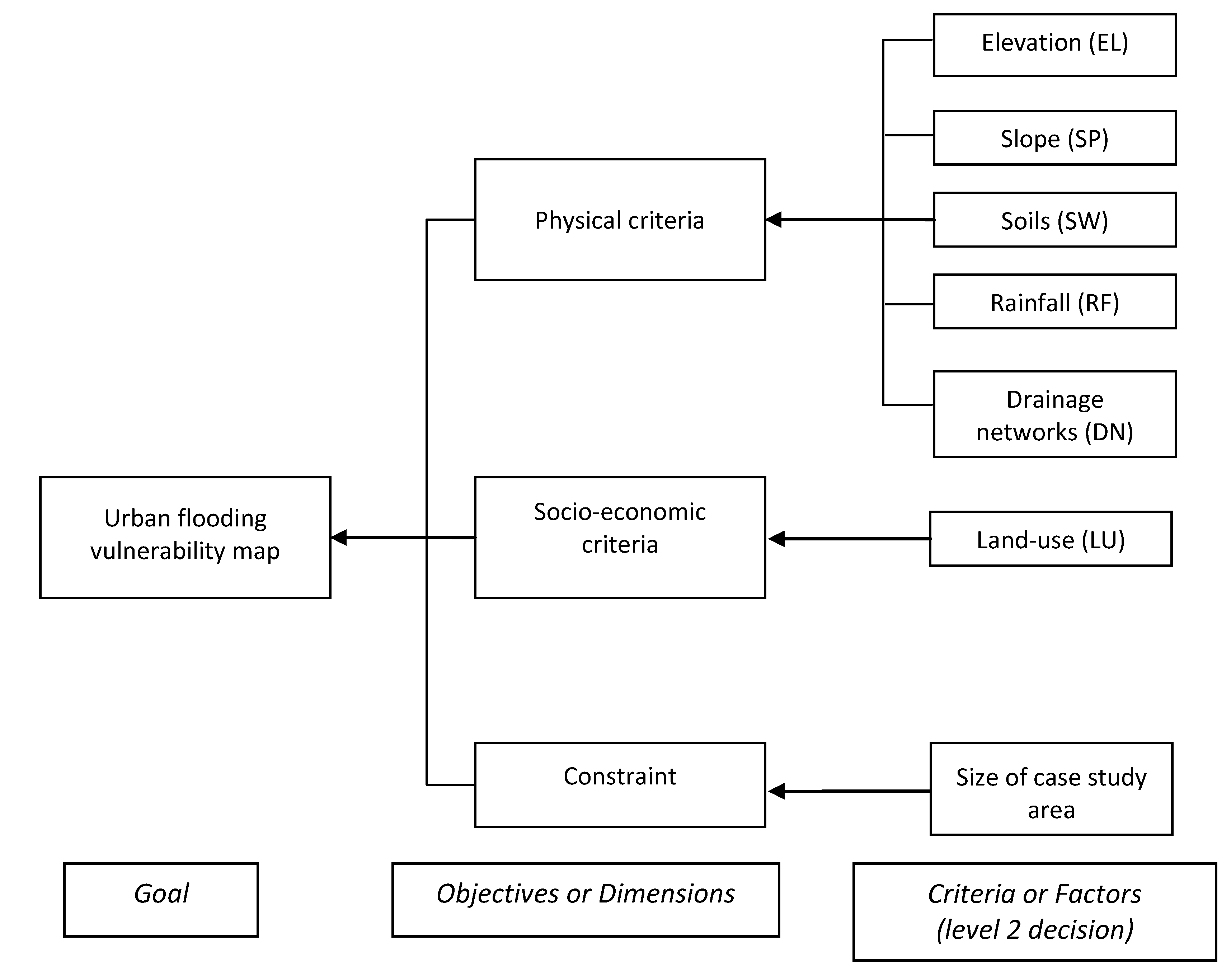
For this case study, a three-level structure was adopted to take into account the physical and socio-economic factors (
Figure 6). These factors as structured in
Figure 6 comprised of: elevation from digital elevation model (EL); slope computed from the DEM (SP); land-use and land-cover from the municipal zoning map (LU); rainfall (RF); soils types (SW) and stream or drainage networks (DN). The municipality boundary is used as a constraint factor in the analysis. Notably, when setting up the AHP hierarchy with a large number of elements, the decision maker should attempt to arrange these elements in clusters so they do not differ in extreme ways as suggested by [
32]. By structuring data in this way (
Figure 6), AHP is used as an Multi-Criteria Decision Analysis (MCDA) in the multi-criteria decision making process.
Figure 6.
A three-level hierarchical structure of the characteristics of the parameters that represents urban flood vulnerability.
Figure 6.
A three-level hierarchical structure of the characteristics of the parameters that represents urban flood vulnerability.
4.2. AHP-GIS Implementation Strategy in Urban Flood Vulnerability Mapping
Flood vulnerability mapping is the process of determining the degree of susceptibility of a given place to flooding. The process involves the selection of bio-physical and/or socio-economic factors of an area; the combination of the selected factors with the decision maker’s preferences allows a user to create a composite suitability index. This process results into a multi-criteria and multi-parametric decision making problem.
To solve such problems, Boolean overlay and modeling approaches such as neural networks and evolutionary algorithms are recently developed methods for performing flood risk mapping in a GIS environment. However, these approaches lack a well-defined mechanism for incorporating the decision maker’s preferences into the GIS procedures. This disadvantage can be solved by integrating GIS and MCE methods, hence producing an effective tool for multiple criteria decision making.
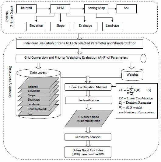
The advantage of MCE is on the integration of a number of choice possibilities in the light of multiple criteria and multiple objectives. An integration of GIS and MCDA can help urban planners and managers to improve decision making processes when it comes to flood vulnerability analysis. This is because GIS enables the computation of assessment factors, while MCE aggregates them into a flood vulnerability index. In this study, GIS was used in the creation of the criteria maps and data layers, spatial analyses and weighting of the AHP evaluated data sets (
Figure 7). This is due to the ability of GIS algorithms to input, store and retrieve, manipulate and analyze, and output spatial and attribute data.
To integrate the AHP with the GIS analysis in the urban flood vulnerability mapping,
Figure 7 presents a schematic outline of the proposed approach. The steps included in
Figure 7 comprises of the primary data used, their manipulation in a GIS environment, multi-criteria decision analysis and model sensitivity analysis. These steps can be categorized as primary and secondary processing stages, with the former being on the processes on data, and the latter being on the algorithmic analysis of the datasets. As depicted in
Figure 7, six different predictor maps were used as structurally represented in the hierarchical structure.
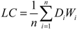
where
LC = linear combination;
Di = decision parameter;
Wi = AHP weight;
n = numbers of parameters.
The most logical and reliable consequence in constructing the vulnerability map was evaluated by the parameters of the study area which are related to given data. In the application of AHP-GIS schema, the parameters concerning the flood risk in the study area have been evaluated and weighted by using the fundamental scale for pairwise comparisons where intensities of 2, 4, 6 and 8 are used to express intermediate values (
Table 1). Theoretically, the values which are close to one have the minimum risk and, similarly, the maximum risky areas have values close to nine. Since the effects of the parameters that are related to disasters are in different proportions, each of them has different input values.
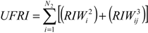
The next step involves the determination of the Relative Importance Weight (
RIW) for each hierarchy element by normalizing the eigenvector of the decision matrix. Finally, an urban flood risk index (UFRI) is computed using GIS overlay analysis as in Equation (6):
where,
N2 = the number of level 2 decision factor;
RIWi2 = relative importance weight of level 2 decision factor
I; and
![Water 06 01515 i014]()
= relative importance weight of level 3 sub-factor
j of level 2 decision factor
i.
Figure 7.
An MCDA conceptual framework for analytical hierarchy process-geographic information system (AHP-GIS) based urban flood mapping and flood risk analysis. The Relative Importance Weight (RIW) is the relative importance weight of the criterion on the different urban land-use classes.
Figure 7.
An MCDA conceptual framework for analytical hierarchy process-geographic information system (AHP-GIS) based urban flood mapping and flood risk analysis. The Relative Importance Weight (RIW) is the relative importance weight of the criterion on the different urban land-use classes.
The UFRI constitutes a simple multi-criteria analysis methodology that can be used as a decision support tool, allowing quantitative rating and comparison between critical flood prone zones. URFI can be useful in the hierarchization of interventions and justification public investments, and in the quantitative comparison of solutions or scenarios for the same region, hence allowing estimating the impacts of future urban development or aiding the elaboration of drainage master plans, among other applications.
UFRI indicators obtained for the different zones of the study area can be plotted as comparative histograms, and based on the set threshold values, the flood risk map of the localized area can be classified into risk classes e.g., “very low”, “low”, “moderate”, “high” and “very high” risk zones.
In this study, the five risk classes were used in ranking, whereby every criterion under consideration was ranked in the order of the decision maker’s preference. To generate criterion values for each evaluation unit, each factor was weighted according to the estimated significance towards causing flooding. The inverse ranking was applied to some of these factors, with weights of 1 being the least important and 5 the most important factor. To make the various criterion maps comparable, a standardization of the raw data is usually required. Linear scale transformation (LST) was adopted as a standardization procedure, since it is able to transform the input data into a commensurate scale [
17]. Using the LST approach, the worst-standardized score was assigned the value 0 and the best score a value of 1.
5. Flood Vulnerability Mapping Variables and Analysis
This section presents the morphometric and topographic elements and variables analysis, as factors in the development of AHP-GIS decision making. Notably, the flood type has major influence on the choice of the variables for the multi-parametric AHP. This section presents the choice of variables used in the vulnerability analysis and their classification into risk classes and intensity of importance (
Table 1). The choice of criterions that has a spatial reference is an important and profound step in multi-criteria decision analysis. Hence, the criteria considered in this study were chosen due to their significance in causing flood in the study area. The factors considered are: elevation and slope; soil types; annual rainfall distribution; drainage density and land-use/land-cover information.
5.1. Elevation and Slope
Elevation and slope play an important role in governing the stability of a terrain. The slope influences the direction of and amount of surface runoff or subsurface drainage reaching a site. Slope has a dominant effect on the contribution of rainfall to stream flow. It controls the duration of overland flow, infiltration and subsurface flow. Combination of the slope angles basically defines the form of the slope and its relationship with the lithology, structure, type of soil, and the drainage. A smooth/flat surface that allows the water to flow quickly is a disadvantage and causes flooding, whereas a higher surface roughness can slow down the flood response. Steeper slopes are more susceptible to surface runoff, while flat terrains are susceptible to water logging.
Low gradient slopes are highly vulnerable to flood occurrences compared to high gradient slopes. Rain or excessive water from the river always gathers in an area where the slope gradient is usually low. Areas with high slope gradients do not permit the water to accumulate and result into flooding. If the main concern is river caused flood, elevation difference of the various DEM cells from the river could be considered, whereas for pluvial flood local depressions, i.e., DEM cells with lower elevation than the surrounding ones, would be more important. This implies that the way in which elevation could be associated with risk is important.
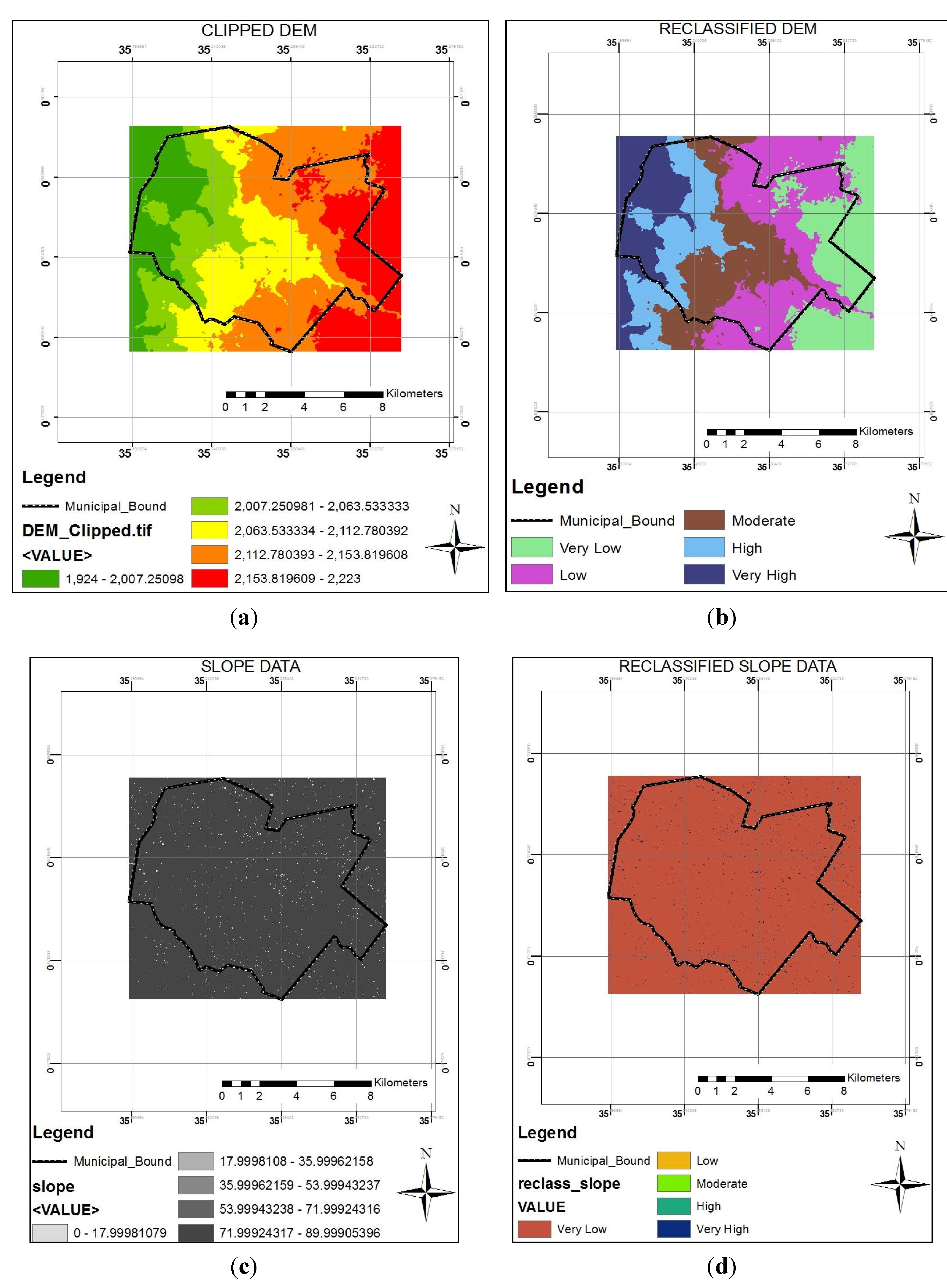
In this study, the slope map was prepared using the digital elevation model (DEM) and slope generation tools in ArcGIS software. The slope classes having less values was assigned higher rank due to almost flat terrain while the class having maximum value was categorized as lower rank due to relatively high run-off. For the case study, the results of the original and reclassified elevation and slope layers are presented in
Figure 8. According to
Figure 8c,d, the entire study area lies in a moderately steep slope. This implies that slope may not be the predominant factor in ranking hazard and risk classes. Note that the upper left corner and lower right corner coordinates of the images generated in
Figure 8a,
Figure 9a,
Figure 10a,
Figure 11a,
Figure 12a,
Figure 13a and
Figure 14a are respectively (0.65° N, 35.14° E) and (0.38° N, 35.39° E).
Figure 8.
Elevation and slope maps: (a) and (c) are the original elevation DEM and slope; while (b) and (d) reclassified elevation and slope maps.
Figure 8.
Elevation and slope maps: (a) and (c) are the original elevation DEM and slope; while (b) and (d) reclassified elevation and slope maps.
Figure 9.
(a) Vector soil layer derived from infiltration rates (mm/hr); and (b) the reclassified soil layer.
Figure 9.
(a) Vector soil layer derived from infiltration rates (mm/hr); and (b) the reclassified soil layer.
Figure 10.
Raster map of: (a) rainfall data; (b) Inverse Distance Weighting (IDW) interpolated rainfall surface and (c) reclassified rainfall data.
Figure 10.
Raster map of: (a) rainfall data; (b) Inverse Distance Weighting (IDW) interpolated rainfall surface and (c) reclassified rainfall data.
Figure 11.
Drainage network depicting: (a) flow accumulation; (b) main rivers derived from the flow accumulation thresholding; (c) drainage density and (d) reclassified drainage density map.
Figure 11.
Drainage network depicting: (a) flow accumulation; (b) main rivers derived from the flow accumulation thresholding; (c) drainage density and (d) reclassified drainage density map.
Figure 12.
(a) Vector map of land-use; and (b) reclassified land-use map.
Figure 12.
(a) Vector map of land-use; and (b) reclassified land-use map.
Figure 13.
Flood hazard map of Eldoret Municipality under modeling.
Figure 13.
Flood hazard map of Eldoret Municipality under modeling.
Figure 14.
(a) Flood vulnerability validation analysis of the AHP-GIS based flood hazard results for the year 2012; (b) Flooding depth under each class from HEC-RAS software simulated and AHP-GIS based results in 2012.
Figure 14.
(a) Flood vulnerability validation analysis of the AHP-GIS based flood hazard results for the year 2012; (b) Flooding depth under each class from HEC-RAS software simulated and AHP-GIS based results in 2012.
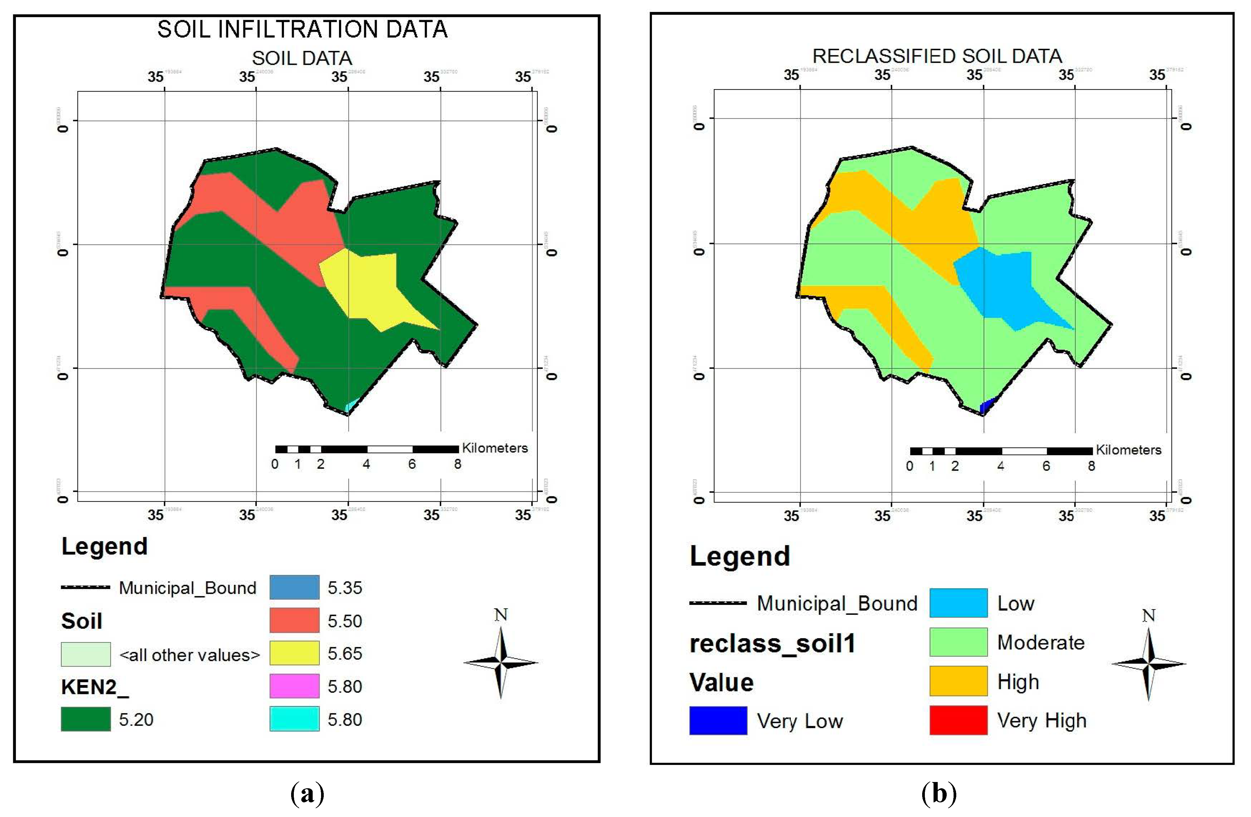
5.2. Soil Type
Soil texture and moisture are the most important components and characteristics of soils. Soil textures have a great impact on flooding because sandy soil absorbs water soon and few runoffs occurs. On the other hand, the clay soils are less porous and hold water longer than sandy soils. This implies that areas characterized by clay soils are more affected by flooding.
Soil moisture can be estimated by the feel and appearance of the soil, whenever not measurements are available. It acts as an interface between the land surface and atmosphere, and plays an important role in partitioning of precipitation into runoff and ground water storage. The levels of soil moisture rise when there is sufficient rainfall to exceed losses to streams and groundwater, and it is important for soil erosion, slope stability as well as the growth for plants and crops. In general, the soil types in an area is important as they control the amount of water that can infiltrate into the ground, and hence the amount of water which becomes flow [
39].
The structure and infiltration capacity of soils will also have an important impact on the efficiency of the soil to act as a sponge and soak up water. Different types of soils have differing capacities. The chance of flood hazard increases with decrease in soil infiltration capacity, which causes increase in surface runoff. When water is supplied at a rate that exceeds the soil’s infiltration capacity, it moves down slope as runoff on sloping land, and can lead to flooding [
40].
For this case study, the soil map was classified on the basis of infiltration capacity. The soil types found within the municipality were considered into the three broad categories: highly infiltrated, moderately infiltrated, and less infiltrated. The soil data for the study area was further vectorized into five infiltration classes, with the results showing that most of the soils study area is of the clay-loam type. The infiltration classes were converted into five raster data groups. The weighted soil map was prepared by assigning weights to each soil classes such that the soil type that has very high capacity to generate very high flood rate is ranked 5 and the one with very low capacity in generating flood rate is ranked 1. The results of the soils factor in the study area are presented in
Figure 9.
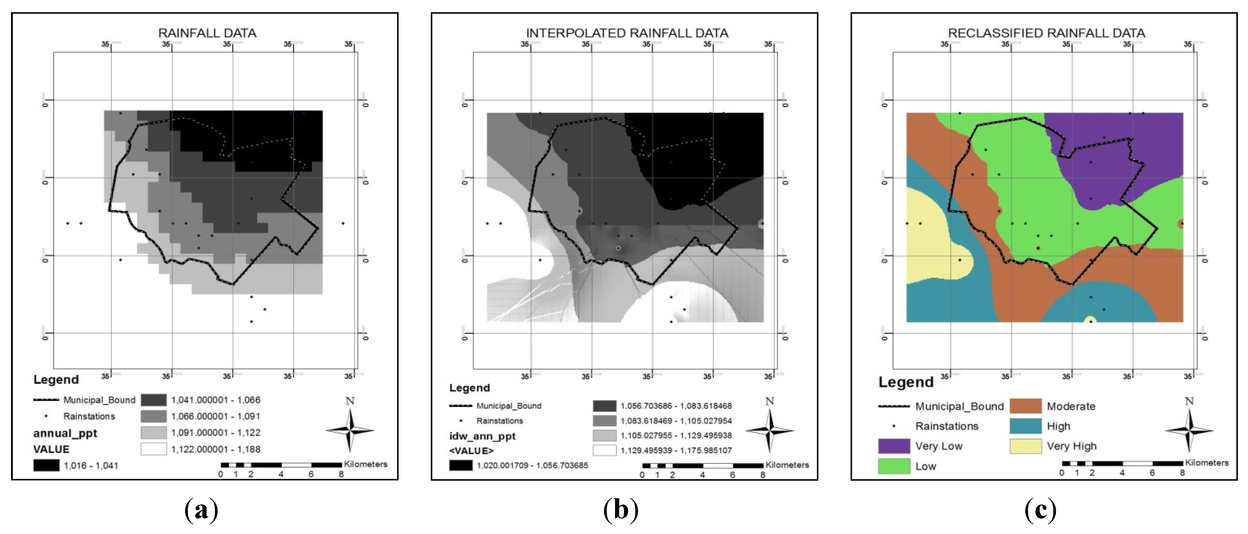
5.3. Rainfall Distribution
Heavy rainfalls are one of the major causes of floods. Flooding occurs most commonly from heavy rainfall when natural watercourses do not have the capacity to convey excess water. Floods are associated with extremes in rainfall, any water that cannot immediately seep into the ground flows down slope as runoff. The amount of runoff is related to the amount of rain a region experiences. The level of water in rivers or lakes rises due to heavy rainfalls. When the level of water rises above the river banks or dams, the water starts overflowing, hence causing river based floods. The water overflows to the areas adjoining to the rivers, lakes or dams, causing floods or deluge.
In the study, it was observed that while the local rainfall is relevant for pluvial flooding, rainfall amounts on the upstream catchments contribute to flood hazard and risk caused by the rivers. Therefore both the local and upstream rainfalls were integrated in the analysis, due to the limited size of the study areas. A mean annual rainfall for eleven years (2001–2011) was considered and interpolated using Inverse Distance Weighting (IDW) to create a continuous raster rainfall data within and around municipality boundary. The resulting raster layer was finally reclassified into the five classes using an equal interval. The reclassified rainfall was given a value 1 for least rainfall to 5 for highest rainfall.
Figure 10 shows the results of the raster rainfall layer, IDW interpolated data layer and the reclassified rainfall data.
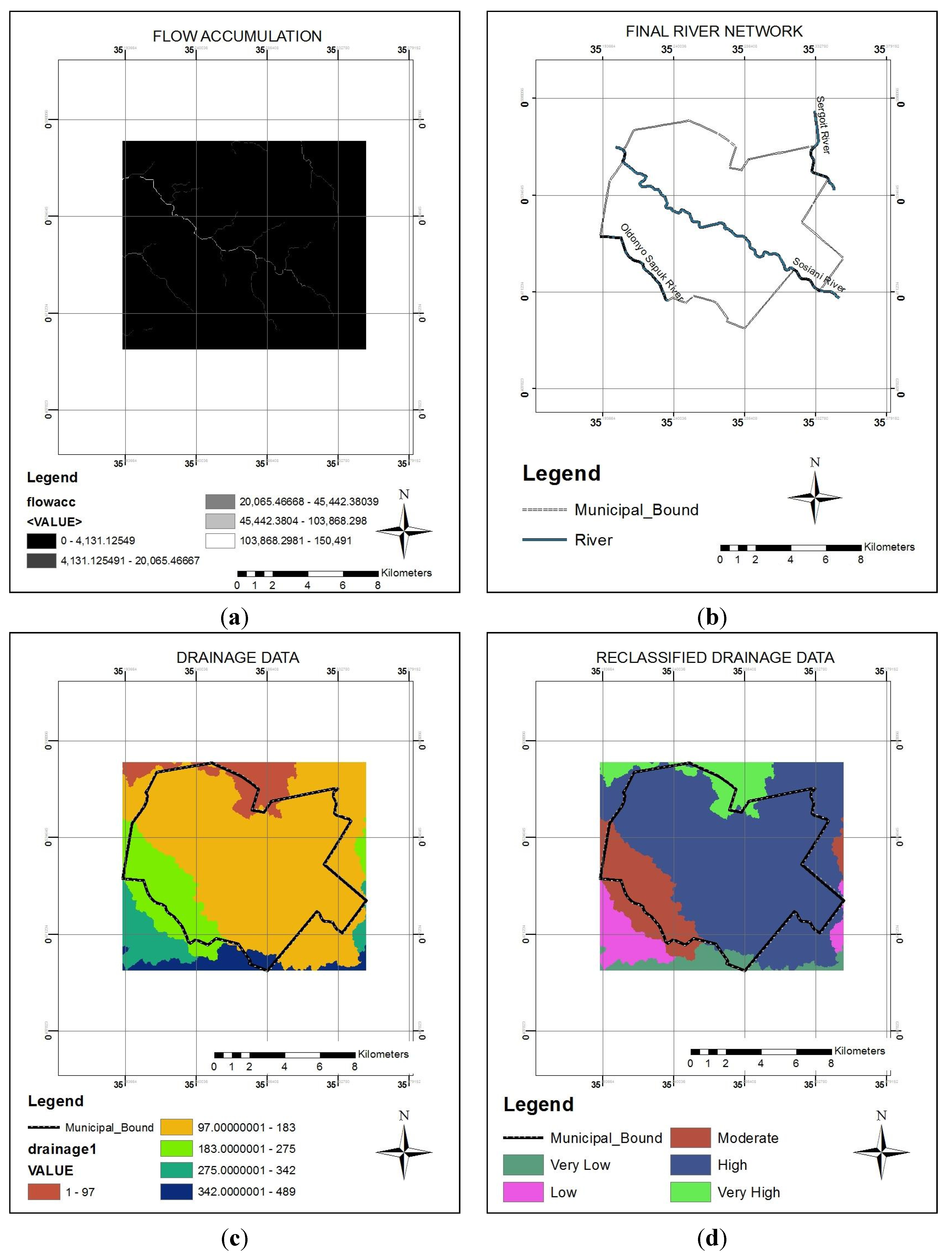
5.4. Drainage Density
Drainage is an important ecosystem controlling the hazards as its densities denote the nature of the soil and its geotechnical properties. This means that the higher the density, the higher the catchment area is susceptible to erosion, resulting in sedimentation at the lower grounds. The first step in the quantitative hazard analysis is designation of stream order. The Stream ordering in the present study area was done using the method proposed by [
41]. Drainage density map could be derived from the drainage map.
i.e., drainage map is overlaid on watershed map to find out the ratio of total length of streams in the watershed to total area of watershed and is categorized. The drainage density of the watershed is calculated as:
D =
L/
A, where,
D = drainage density of watershed;
L = total length of drainage channel in watershed (km);
A = total area of watershed (km
2).
A watershed with adequate drainage runoff should have a drainage density ≥ 5, whilst the moderate and the poor ones have drainage density classes 1–5 and <1 respectively. In the study area, streams of up to 2nd order were noted. For the study area, higher weights were assigned to poor drainage density areas and lower weights were assigned to areas with adequate drainage.
From the flow accumulation of the study area, three main rivers in the study area were derived: Sosiani, Oldonyo-Sapuk and Sergoit Rivers (
Figure 11). The drainage density layer was further reclassified in five sub-groups using the standard classification Schemes (1–5). Areas with very low drainage density are ranked as 5 and those with very high drainage density were ranked with value of 1 as depicted in the results
Figure 11.
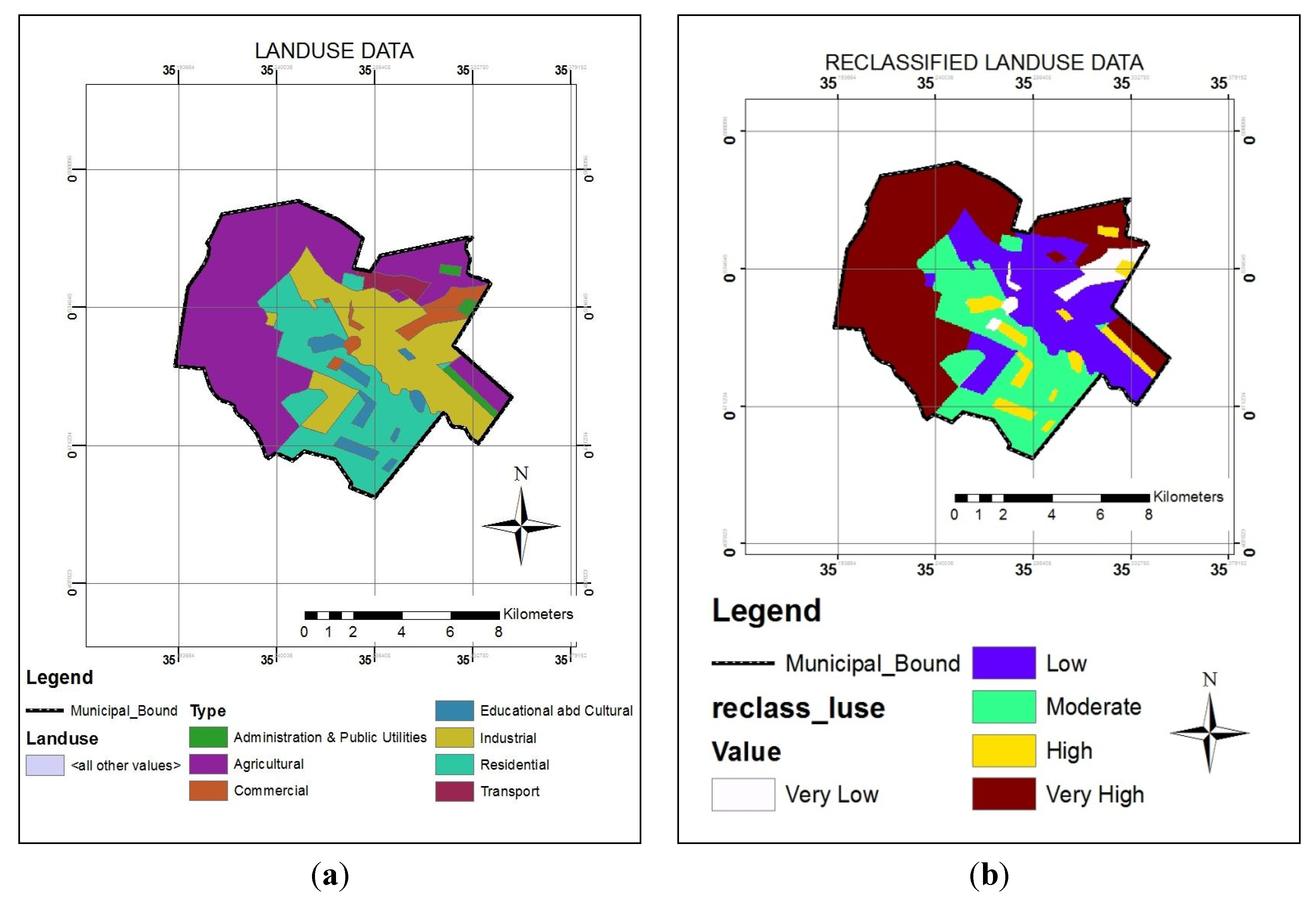
5.5. Land-Use and Land-Cover Criteria
The land-use and land-cover management of an area is also one of the primary concerns in flood hazard mapping because this is one factor which not only reflects the current use of the land, pattern and type of its use but also the importance of its use in relation to soil stability and infiltration.
Land-cover like vegetation cover of soils, whether that is permanent grassland or the cover of other crops, has an important impact on the ability of the soil to act as a water store. Runoff of rainwater is much more likely on bare fields than those with a good crop cover. The presence of thick vegetative cover slows the journey of water from sky to soil and reduces the amount of runoff. On the other hand, impermeable surfaces such as concrete, absorbs almost no water at all. Land-use like buildings, roads, slum areas, decreases penetration capacity of the soil and increases the water runoff. In other words, land-use types work as resistant covers and decrease the water hold up time; and typically, it increases the peak discharge of water that enhances a fastidious flooding. This implies that land-use and land-cover are crucial factors in determining the probabilities of flood happenings.
The land use land cover classes of the study area were prepared from the municipal zoning maps. Zoning based land-use map of the study area was reassigned by categorizing the land-use types into six general classes and converted to raster layer. The existing land-use classes of the area were reclassified into five groups in order of their capacity to increase or decrease the rate of flooding. The results of the land-use/land-cover data analysis are shown in
Figure 12.
6. Results and Discussions
6.1. Ranking of Flood Mapping Criteria
The ranking and prioritization process is the main purpose of AHP based multi-criteria decision making. The quality of priority-setting directly influences the effectiveness of available resources which are, in most cases, the primary judgment of the decision maker. When making decisions, hydrologists and engineers frequently use heuristic and experiential judgments from the public who are the end-users.
In this study, to determine the objectives and formulate the decision making process, sixteen experts comprising of four hydrologists, four engineers and eight end-users were asked to give their assessments and judgments regarding the variables related to flooding and their significances in terms of weights, out of the six factors analyzed. Experts or decision makers comprise of those with the technical skills and know-how for solving a given problem, while end-users are the public who are affected by the phenomenon and for this case study comprised of representatives from community leaders, area chief and sub-chief. Each of the expert participants assigned weights to the objective factors in three rounds, with each round using a different approach comprising of the following rounds:
Round 1: Assign each objective or factor a percentage to indicate the weight;
Round 2: Use round 1 to indicate the lowest importance, and assume the importance scale among the objectives is linear;
Round 3: The importance of objectives should be ranked using a 1 to 5 scale, with 1 representing the least important and 5 representing the most important.
In order to illustrate the significance of each factor as compared to the other criteria in resulting flood hazard, eigenvector is used to weight the standardized raster layers. The results of the pairwise comparison and ranking of the criterion are presented in
Table 3. Next,
Table 4 shows the normalized matrix converted to percent contributions, from which the average priority vector (
X) is derived.
Table 3.
Ranking of urban flood causing criteria to obtain the pairwise comparison matrix.
Table 4.
Normalizing the criteria columns to obtain the normalized matrix.
Table 4.
Normalizing the criteria columns to obtain the normalized matrix.
| Normalized Matrix |
|---|
| Criteria | Rainfall | Drainage | Elevation | Slope | Soil | Land-use | Priority vector (X) | Percent (%) |
|---|
| Rainfall | 2/13 | 2/13 | 2/13 | 2/13 | 2/13 | 2/13 | 0.1301 | 13% |
| Drainage | 2/13 | 2/13 | 2/13 | 2/13 | 2/13 | 2/13 | 0.0814 | 8% |
| Elevation | 3/13 | 3/13 | 3/13 | 3/13 | 3/13 | 3/13 | 0.0710 | 7% |
| Slope | 4/13 | 4/13 | 4/13 | 4/13 | 4/13 | 4/13 | 0.1800 | 18% |
| Soil | 1/13 | 1/13 | 1/13 | 1/13 | 1/13 | 1/13 | 0.2771 | 28% |
| Land-use | 1/13 | 1/13 | 1/13 | 1/13 | 1/13 | 1/13 | 0.2604 | 26% |
| Total | 1 | 1 | 1 | 1 | 1 | 1 | – | 100% |
From
Table 4, the consistency check
CI is determined from the matrix formulation (
AX = λ
maxX); where (
A) is the pairwise matrix and (
X) is the eigenvector of weights. From the solution for λ
max, the
CI is obtained as in Equation (7):
with
n =
N = 6 decision factors.
Finally the consistency ratio is computed from:
CR =
CI /
RI = 0.11/1.24 = 0.09, with
RI obtained from
Table 2. The obtained
CI is much lower than the threshold value of 0.1 and indicates a high level of consistency in the pairwise judgments, and implies that the determined weights are acceptable. The computed eigenvector is used as a coefficient for the respective factor maps to be combined in the weighted overlay.
6.3. Flood Vulnerability Mapping for Eldoret Municipality
Once the weights for the factors are determined, a multi-criteria evaluation is performed by utilizing the specific weights for each factor, the factors themselves, and the constraint maps for each factor to produce the flood prediction mapping. To derive the flood vulnerability map, a weighted linear combination (LC) overlay of the decision factors according to Equation (5) in
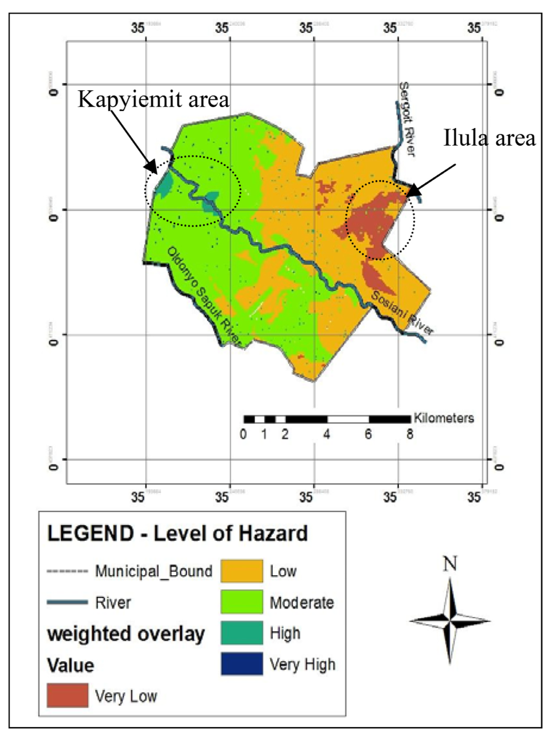
Figure 7 is used as depicted in
Figure 7. The result is a flood vulnerability or hazard map showing the most vulnerable areas to flooding within the municipality. The results of this stage of analysis are shown in
Figure 13.
The results show that almost a fifth of the total municipal area was prone to “high” and or “very high” flood hazards. These areas are those that are close to the rivers and generally laying at low elevations within the settled/paved regions. Conversely, four-fifths of the study area was prone to “very low” to “moderate” level of flood hazards. Most of these areas tended to be on the higher grounds and further away from the high drainage density areas. Significantly, the results in
Figure 13 depict the fact that Eldoret Town’s central business district (CBD) is prone to “moderate” flooding vulnerability. This is due to the fact that despite the CBD having drainage networks, most of them are clogged and coupled with the fact that the urban paved surfaces hinder water infiltration of runoff, these areas are prone to flooding events during heavy rainfall occurrences.
As the multi-parametric and multi-criteria analysis forms a single map from the combination of all analyzed map, then the final output (
Figure 13) will represent the desired result for flood prediction map for the duration of study.
6.4. Results Validation Using Flood Area Extent and Depths
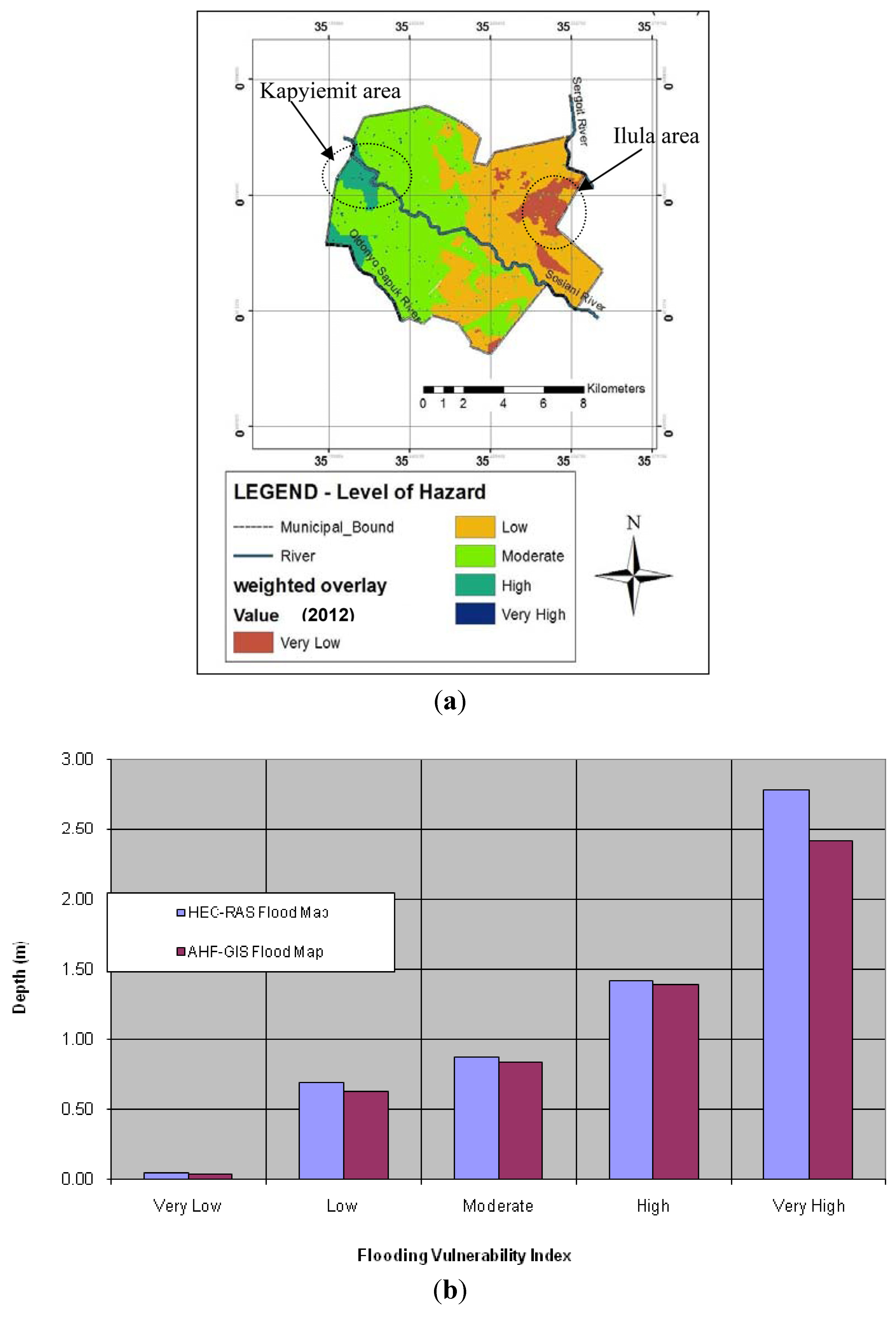
To perform the validation of the flood zonation results, flooding-based field verification was carried out at twenty verification areas evenly distributed within the five vulnerability classes derived in
Figure 13 for the year 2012. Both the flood area extents and depths were used in the validation process. HEC-RAS was used to simulate the flood map through interpolation of the observed flood depths. The HEC-RAS simulation procedure follows the following steps: (a) the geometric data from a Triangulated Irregular Network (TIN), derived from DEM is extracted using ArcGIS for use in the HEC-RAS model; (b) the HEC-RAS model is built by inputting depth data previously created from a HEC-Hydrologic Modeling System (HMS) model. Steady-state simulations are run to generate water depth surface profiles; and finally (c) by exporting the HEC-RAS model results into ArcGIS the simulated flood maps are created, for comparison with the flood vulnerability map (modeled from the actual physical parameters). The depths are then compared in verification each area so as to determine the “true positive” and “false positives”.
For the flood area extent, the 2012 results in
Figure 14a compared to the ground measurements showed that 5.14% and 7.87% of the total area was erroneously classified as vulnerable to very high and high flood hazard zone respectively. An average error of 4.06% of the total area was found to be the least vulnerable (“low” to “very low”) to flood hazard. The results depict the fact that the maximum error probability of zoning an area to be prone to any of the flood scenarios, when it is actually not,
i.e., false positive is not more than 8%.
The simulated HEC-RAS flood map and the averages for each vulnerability classes in
Figure 14a were compared. Comparing the simulated flood phenomenon and the actual field measurements for the flood occurrences in
Figure 14a, the results in
Figure 14b showed that a minimum average difference of 0.01 m and a maximum average difference of 0.37 m in flood depths were observed. The results shows the simulated results were generally higher than the AHP-GIS based values, with the highest depths differences being in river located verification flooding points.
6.5. Urban Flood Risk Index (UFRI) Mapping
The determination of flood risk areas is normally accomplished through subjective and even intuitive approaches, with the concept of risk itself interpreted in a variety of ways. Frequently, FRI analysis only takes into account the flood depth or the affected population, leaving aside other aspects that knowingly affect the gravity of the problem. Also, in these evaluations, it is unusual to make any distinction between the relative importance of each constituting factor.
Consequently, risk assessment traditionally should result in the simple identification of critical zones (presence/absence), hence hampering comparisons between them or restricting the study of individual management alternatives for in depth analysis of the urban flooding problems according to the different land-use zones within the municipality. This approach formulates the urban flood risk index.
For this study, the urban flood risk index was derived for the five main land-use classes within the municipality. The result in
Table 6 shows that the residential areas in Eldoret Municipality are were more susceptible to flooding, while the least vulnerable are those occupied by administrative and public utilities. This can be attributed to lower infiltration in these areas and also due to lack of proper drainage networks especially in poor planned and informal-overpopulated urban settlements. On the other hand, the agricultural areas are not very vulnerable due to the higher infiltrations and soil cover.
Table 6.
Land-use flood risk index (FRI) within Eldoret Municipality.
Table 6.
Land-use flood risk index (FRI) within Eldoret Municipality.
| Urban land-use factors | Relative weight of level 3 sub-factor (j) of level 2 decision factor (i) = ( ![Water 06 01515 i014]() ) ) | ![Water 06 01515 i013]() |
|---|
| Agricultural | 0.28 | 30.1% |
| Industrial and Commercial | 0.21 | 22.6% |
| Residential | 0.43 | 34.1% |
| Administration and Public Utilities | 0.02 | 10.5% |
| Educational and Cultural | 0.06 | 2.7% |
6.6. Further Discussion of Results
Determining the flood vulnerable areas as carried out in this study is important for decision makers for planning and management activities. Traditionally, hydrologic/hydraulic models are commonly used to assess the potential areas of inundation and flood damage for given recurrence intervals. In essence, these models are only based on the balance of the flow and the conveyance of waterways. The flood vulnerability assessment applied in this study consists of two basic phases. Firstly, the effective factors or variables causing floods are determined. Secondly AHP based MCE in a GIS environment is applied and these approaches are evaluated in finding the flood vulnerable areas. The results are extended to determine the flood risk index for the different urban zones. Such approach may be more pragmatic than the hydraulic-only models, and integration of the two approaches is recommended.
From the study results, it is observed that AHP offers a flexible, step-by-step and transparent way of analyzing complex problems in a MCDA environment—based on experts and end-user preferences, knowledge, and judgments. In fact, the resolution of complex problems in a multi-criteria environment is seen as the primary use of AHP. In this case study where slope, elevation, rainfall, soils, land-use/land-cover and localized drained density have different dimensions, makes a simple MCDA problem more complex. In a typical MCDA situation, where multiple criteria and different fields are involved, there is a need to consider multiple stakeholders and wide-ranging expertise. Owing to its ability to readily incorporate multiple judgments, AHP and its combination with other tools such as GIS offer a solution to multi-dimensional and multi-parametric complex problems. Indeed, the application of AHP as a decision support tool or weighting method for GIS-based MCDA marks its potential usefulness to wider applications where multi-parametric geospatial analysis is involved.
Further, the AHP-GIS based approach to flood risk assessment as applied in this study is seen as a relatively inexpensive, easy to use, and more importantly, allows interactive use by flood managers for continuing improvement. This is because the AHP rating indices and numerical results can be used by flood managers as a reference for flood control planning and flood defense. Nonetheless, AHP has its own problems and challenges. For example, data used for analyzing flood risk are normally derived from different sources, in different formats, periods and resolutions. Therefore, it may be difficult to standardize the datasets for evaluating the flood risk. This however may not significantly affect the quality of ranking the flood causative factors because these criteria are weighted differently.
Review-wise, researchers have still not reached a consensus on some issues related to the implementation of AHP as a weighting method for GIS-based MCDA. The contentious areas include: (i) the method for capturing experts’ opinions using the pairwise comparison method; (ii) the method for aggregating individual expert ratings (in cases where consensus ratings are not used); and (iii) the method for standardizing the criteria or factors involved in the analysis. Nevertheless, the AHP method has received considerable attention because it also places greater emphasis on the structure of the preferences of the decision makers.


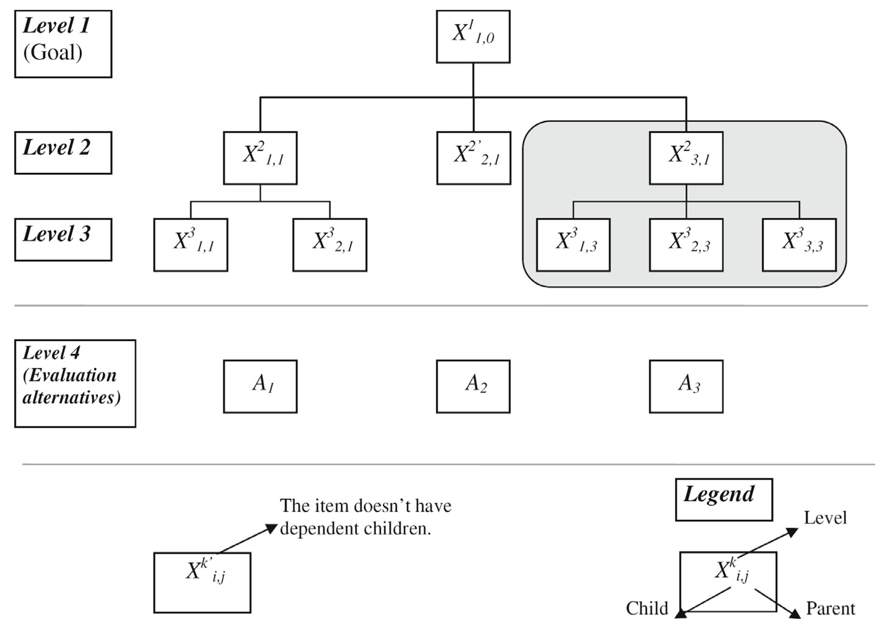
 , where i is the order of the child at the level/layer k, and j is the parent of the child [38]. For example,
  represents the item is at level k = 2, is the first child i = 1 and its parent is j = 1. Each child, in the intermediate levels, is criterion and sub-criterion that affect the corresponding parent and child, respectively. The apostrophe on any intermediate item (element, factor, sub-criterion),
  , indicates that the element does not have dependent children. The ensuing derivation and discussions are limited to the shaded items located at levels 2 and 3 (i.e.,
  ).
).
 = relative importance weight of level 3 sub-factor j of level 2 decision factor i.