Article

Comparison of Performance between Genetic Algorithm and SCE-UA for Calibration of SCS-CN Surface Runoff Simulation

1
Department of Environmental Engineering, Andong National University, Andong 760-748, South Korea
2
Department of Rural Construction Engineering, Kongju National University, Yesan 340-702, South Korea
3
Department of Agricultural and Biological Engineering, Purdue University, West Lafayette, IN 47907-2093, USA
*
Author to whom correspondence should be addressed.
Water 2014, 6(11), 3433-3456; https://doi.org/10.3390/w6113433
Submission received: 14 July 2014 / Revised: 4 November 2014 / Accepted: 6 November 2014 / Published: 12 November 2014

Abstract

:
Global optimization methods linked with simulation models are widely used for automated calibration and serve as useful tools for searching for cost-effective alternatives for environmental management. A genetic algorithm (GA) and shuffled complex evolution (SCE-UA) algorithm were linked with the Long-Term Hydrologic Impact Assessment (L-THIA) model, which employs the curve number (SCS-CN) method. The performance of the two optimization methods was compared by automatically calibrating L-THIA for monthly runoff from 10 watersheds in Indiana. The selected watershed areas ranged from 32.7 to 5844.1 km2. The SCS-CN values and total five-day rainfall for adjustment were optimized, and the objective function used was the Nash-Sutcliffe value (NS value). The GA method rapidly reached the optimal space until the 10th generating population (generation), and after the 10th generation solutions increased dispersion around the optimal space, called a cross hair pattern, because of mutation rate increase. The number of looping executions influenced the performance of model calibration for the SCE-UA and GA method. The GA method performed better for the case of fewer loop executions than the SCE-UA method. For most watersheds, calibration performance using GA was better than for SCE-UA until the 50th generation when the number of model loop executions was around 5150 (one generation has 100 individuals). However, after the 50th generation of the GA method, the SCE-UA method performed better for calibrating monthly runoff compared to the GA method. Optimized SCS-CN values for primary land use types were nearly the same for the two methods, but those for minor land use types and total five-day rainfall for AMC adjustment were somewhat different because those parameters did not significantly influence calculation of the objective function. The GA method is recommended for cases when model simulation takes a long time and the model user does not have sufficient time for an optimization program to search for the best values of calibration parameters. For other cases, the SCE-UA program is recommended for automatic model calibration.

1. Introduction

Recently, optimization techniques have become widely used in computer modeling applications. A major advantage of the application of optimization techniques with models is to obtain better results without significant effort and time. Optimization techniques can be divided into two groups: global search methods such as Genetic Algorithm (GA) [1] and Shuffled Complex Evolution (SCE-UA) [2] algorithm, and local search methods, such as the downhill simplex method [3], the pattern search method [4], and the rotating direction method [5]. Numerous studies have reported that global search methods performed better than local search methods [6,7,8,9,10].
Numerous studies reported that the SCE-UA algorithm provided better estimates of the solution compared with other global and local search procedures for calibrating watershed models. Cooper et al. [6] evaluated three global optimization methods including the SCE-UA, GA and simulated annealing (SA). They found that the performance of optimization was influenced by the objective function and starting position of the optimization search, and the SCE-UA method provided better results compared with other methods. Franchini et al. [8] reported that the solutions from SCE-UA were stable but characterized by many parameter values set at the boundary of their potential range. Kuczera [11] indicated the reason the SCE-UA is better than GA due to the periodic global sharing of information between the local simplex searches. Thyer et al. [10] revealed that SCE-UA’s use of multiple complexes and shuffling provided a more effective search of the parameter space than GA’s single simplex.
Although most optimization applications for automated model calibration continue to be studied, recent research activity in optimization for environmental modeling is centered on systematic analysis and selection of the best alternative for environmental management strategies. Vasques et al. [12] applied GA with the first-order reliability method (FORM) for estimating the probability of system failure under a given wasteload allocation to achieve wasteload allocation solutions between treatment cost and reliability. Ngo et al. [13] proposed to optimize control strategies for reservoir operation by applying SCE-UA methods. Kerachian and Karamouz [14] identified operating rules for water quality management in reservoir-river systems using a stochastic GA based conflict resolution technique. Park et al. [15] proposed application of an optimization method for effective water quality monitoring in a large river system.
New optimization algorithms have been developed and some algorithms demonstrated better capability than GA or SCE-UA for some problems [16,17]. However, GA and SCE-UA algorithms are applied for automatic calibration and determination of alternative strategies for watershed management, while other researchers have enhanced algorithm capabilities. Table 1 summarizes case studies of GA and SCE-UA application over the last five years (2010–2014) [18,19,20,21,22,23,24,25,26,27,28,29,30,31,32,33,34,35,36,37,38,39,40,41,42,43,44,45,46,47,48,49,50,51,52,53,54,55,56,57,58,59,60,61,62,63]. SCE-UA has been primarily applied for automatic calibration, while GA has been more widely used for decision-making associated with watershed management strategy.
Table 1. Case studies of GA and SCE-UA algorithm application for the last five years (2010–2014).
Case StudyGASCE-UA
Automatic calibration9 [18,19,20,21,22,23,24,25,26]19 [40,41,42,43,44,45,46,47,48,49,50,51,52,53,54,55,56,57,58]
Decision making11 [27,28,29,30,31,32,33,34,35,36,37]2 [59,60]
Algorithm enhancement2 [38,39]3 [61,62,63]
Therefore, GA and SCE-UA can be expected to be widely used for watershed and water quality management for selection of the best alternatives for management as well as automated model calibration. In this study, GA and SCE-UA methods coupled with the Long-Term Hydrologic Impact Assessment (L-THIA) model, which employs the curve number (CN) method, were applied to 10 watersheds. The two optimization methods were characterized by analyzing how they generated solution populations and found optimal values according to the number of iteration of model runs. This study might help for user to select between GA and SCE-UA or for developer to improve the algorithm.

2. Theoretical Background

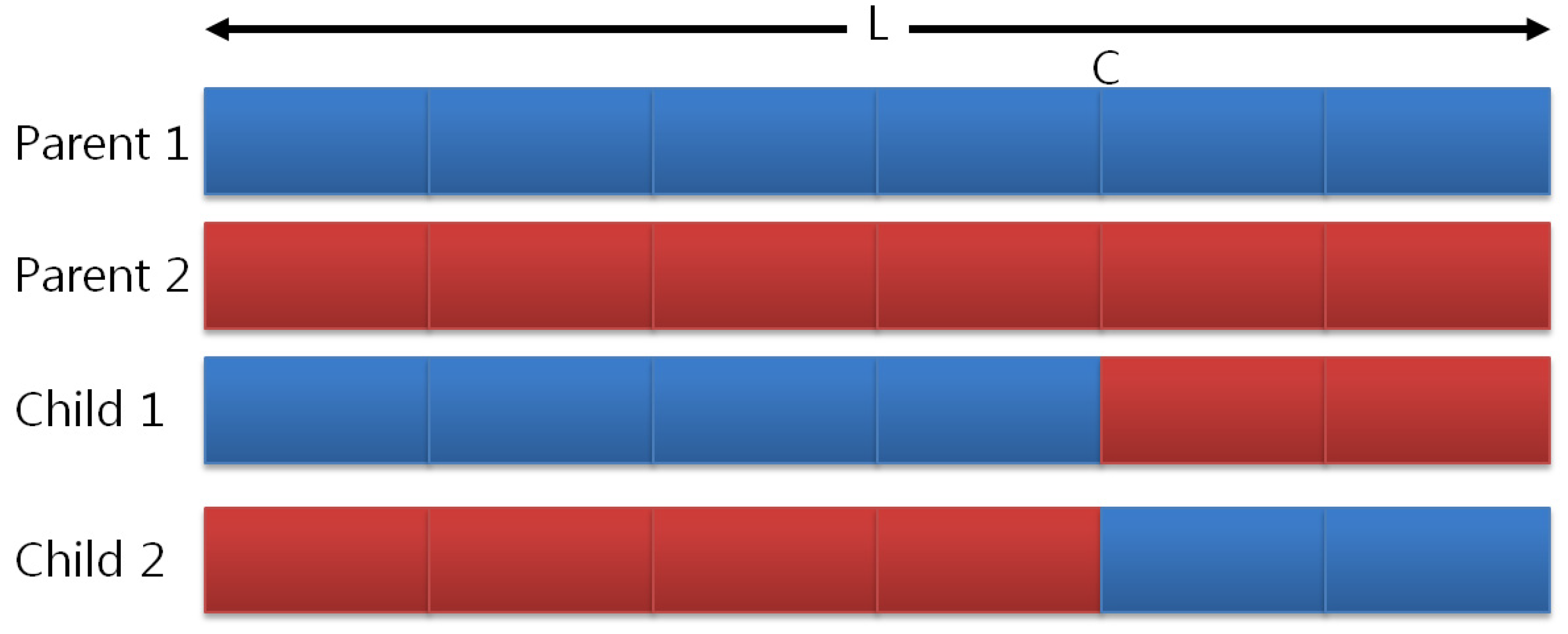
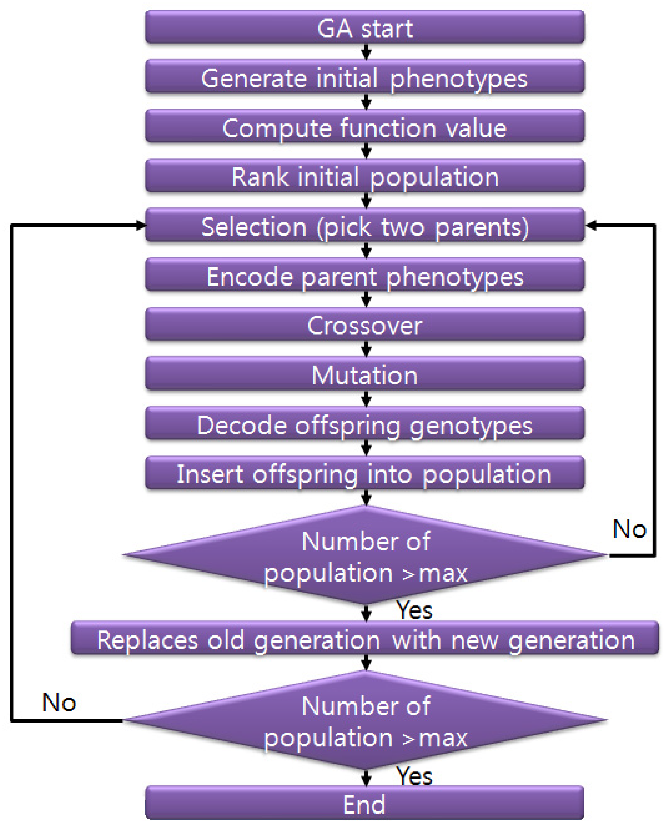
2.1. Genetic Algorithm (GA)

The GA is based on the principle of natural selection and natural genetics combining an artificial survival of the fittest with genetic operators abstracted from nature [1]. The GA method employs three distinct operations including reproduction, crossover, and mutation, which make the initial population to be evolved the next generation [64]. The flow chart of the PIKAIA version 1.0, which is a self-contained, genetic-algorithm-based optimization subroutine developed at the High Altitude Observatory [65], is shown in Figure 1. The initial population of chromosomes is generated randomly, and the objective functions for each individual are calculated. Both parents in one iteration of the reproductive cycle are selected by PIKAIA’s stochastic sampling mechanism for new individual generation. A chromosome-like structure for each selected parent is produced for use in crossover and mutation processes. One-point crossover between a pair of parent-individuals is implemented to create a pair of offspring-individuals. One-point crossover selects randomly point C in length L and exchanges the codes of the pairs as shown in Figure 2. Mutation is implemented here by exchanging the values of some randomly chosen grid cells within one parent. The most-fit individuals are selected to mate and reproduce. The procedures from generating an initial population to select to mate and reproduce are repeated until a specific condition is met. Please refer the user guide of PIKAIA 1.0 for more detailed information [65]. In this procedure, the population of chromosomes or individuals is a group of generated values for an optimized parameter, and parents are selected values within the group based on the objective function in the hydrologic model.
Figure 1. Flow chart of GA PIKAIA technique.
Water 06 03433 g001
Figure 2. One-point crossover method [64].
Water 06 03433 g002

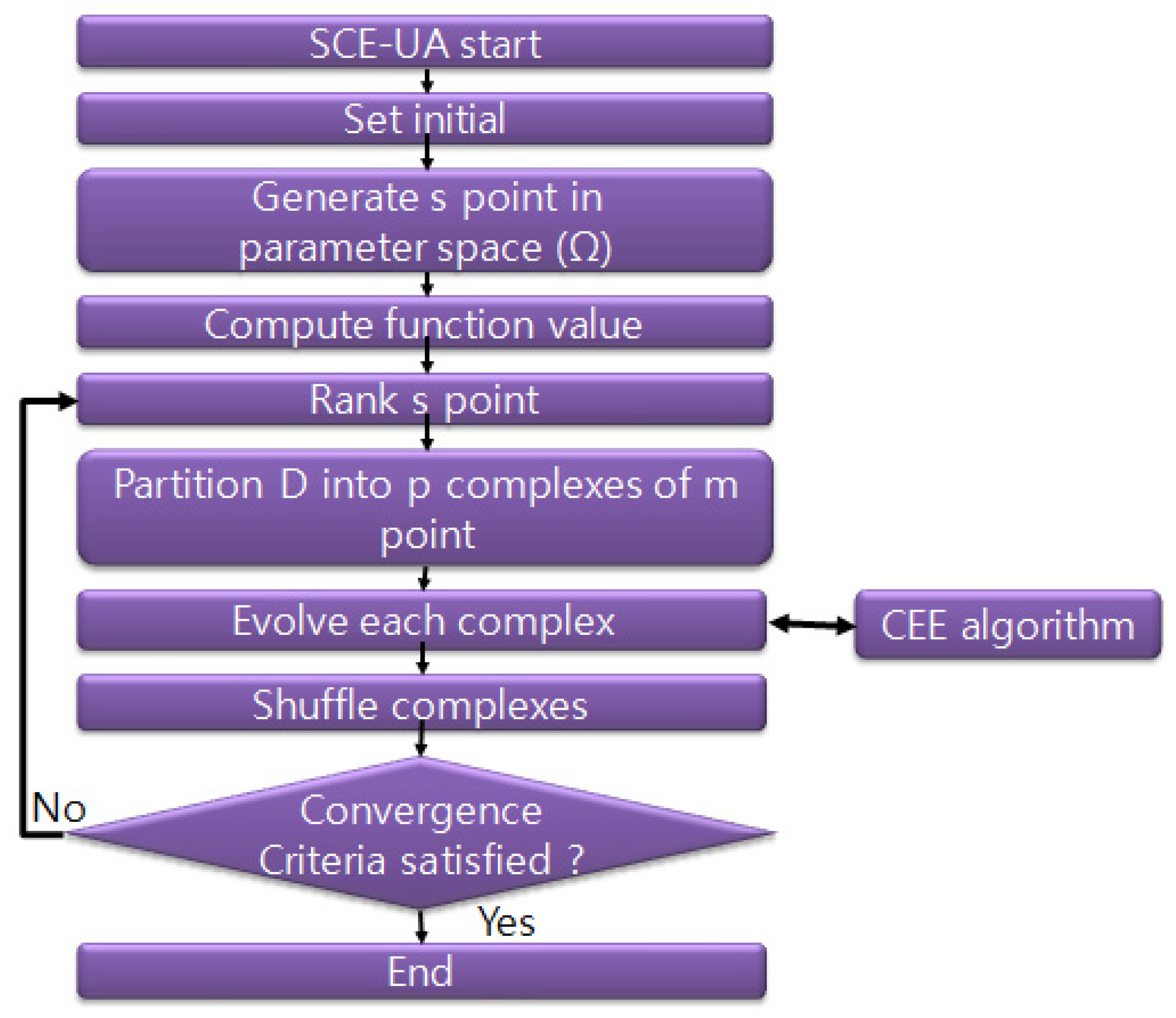
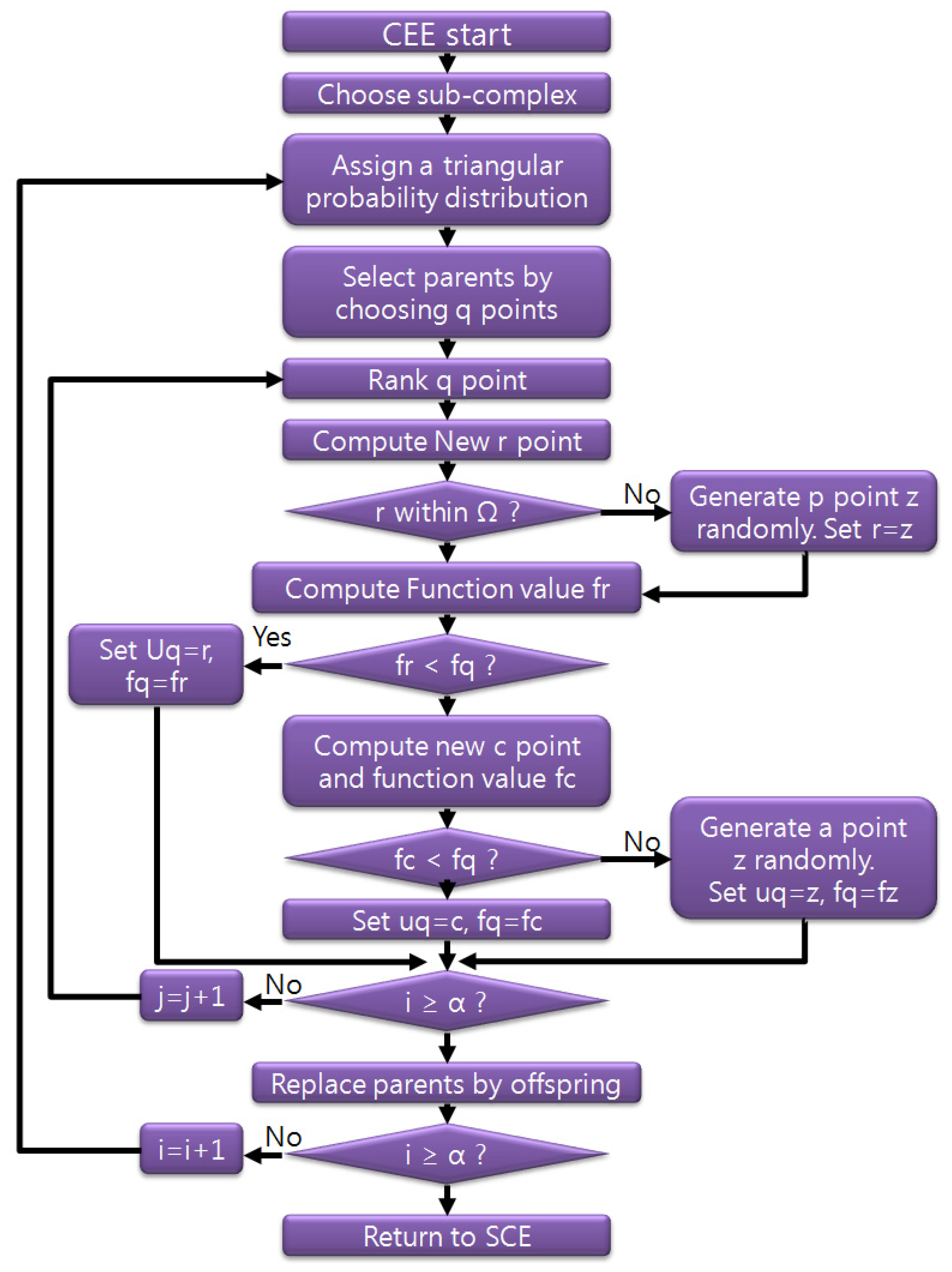
2.2. Shuffled Complex Evolution (SCE-UA)

The SCE-UA was developed in the Department of Hydrology and Water Resources of the University of Arizona and combined the simplex procedure with the concept of controlled random search [3], competitive evolution [1], and a complex shuffling concept [2]. The SCE-UA flow chart is illustrated in Figure 3. Number of complexes (p) and points (m) in each complex are initialized and sample size is s = p × m. s points are generated in parameter spaces randomly; function values are calculated at each s points; and s points are ranked from the worst criteria value to the best criteria. The s points are partitioned into p complexes containing m points in partitioning into complexes. Each complex is evaluated according to the competitive complex evolution (CCE) algorithm outlined separately. The sample population is sorted, and the sample population is shuffled into p complexes. Convergence and the reduction in the number of complexes are checked. In the CCE algorithm, each complex is evaluated and is illustrated in Figure 4. In this procedure, s points are a group of generated values for an optimized parameter, and function values are calculated from the objective function between observations and hydrologic model simulation values.
Figure 3. Flow chart of SCE-UA algorithm [2].
Water 06 03433 g003

2.3. Long-Term Hydrologic Impact Assessment Model (L-THIA)

The L-THIA model was developed to evaluate the impact of land use change and long-term characteristics of watershed hydrology and nonpoint source pollution by combination of CN and event mean concentration (EMC) methods [66]. The L-THIA model is available as a GIS version (Figure 5) and Web-L-THIA version available [67]. The L-THIA model is primarily used in watershed management to simulate various hydrologic conditions for land use change [68,69,70,71] and loads of various nonpoint source pollution [72,73,74]; evaluate various scenarios for land use management [75,76]; develop total maximum daily loads (TMDLs) [77]; and evaluate low impact development (LID) [78,79,80].
Figure 4. Flow chart of CCE subroutine in SCE-UA algorithm [2].
Water 06 03433 g004
Figure 5. Overview of GIS L-THIA application [66].
Water 06 03433 g005

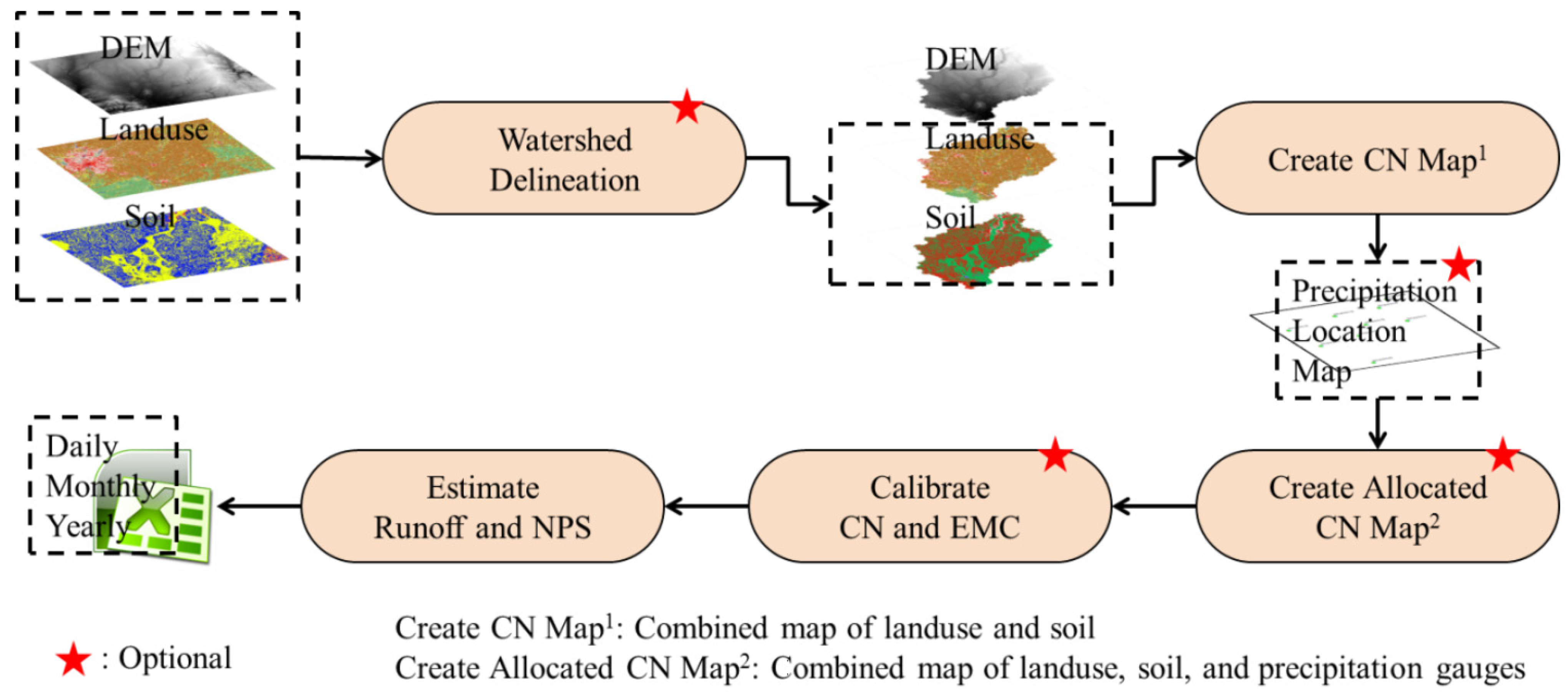
3. Materials and Methods

SCE-UA and GA were linked to the L-THIA model for automated calibration of surface runoff. Ten watersheds in Indiana were selected and calibrated for surface runoff for comparison of the two methods. CN values and amount of total 5-day rainfall for antecedent moisture condition (AMC) adjustment were calibrated automatically using an approximately 10-year calibration period for each watershed. During the automated calibration process, the generated individuals and their objective values were extracted and compared to review how each optimization method searches for the optimal value by using various graphical techniques. Calibrated CN values and 5-day rainfall for AMC adjustment from the two methods were graphically plotted.

3.1. Modeling Approach

CN value is assigned to the combination of land use type and hydrologic soil group. For more exact simulation, spatial rainfall distribution needs to be considered by L-THA for runoff simulation. Thiessen polygons for rainfall gages, land use classification, and hydrologic soil group layers were overlapped and CN values were assigned for each Thiessen polygon area. The surface runoff for different Thiessen polygon areas were simulated separately and summed. The L-THIA model predicted runoff based on daily simulation by considering AMC classification and the objective function was calculated monthly because the L-THIA model does not consider routing processes since the main application of the L-THIA model is for long-term simulation. The Nash-Sutcliffe (NS) coefficient is widely used for evaluating hydrological simulation performance [81] and was used as the objective function in this study:
N S = 1 i = 1 N ( Q o b s , i Q s i m , i ) 2 i = 1 N ( Q o b s , i Q _ o b s , i ) 2
where Qobs is the observed direct runoff; Qsim is the simulated direct runoff; and Q _ obs is average observed direct runoff.

3.2. Optimization Approach

FORTRAN codes of GA for PIKAIA version 1.0 and SCE-UA for version 2.2 were used to develop automated calibration of the L-THIA model. In each subroutine, which calculates the objective function of the two optimization programs, the surface runoff was simulated by an L-THIA algorithm, and the objective function value was calculated using simulated and observed runoff data.
AMC is divided as AMC I for dry conditions, AMC II for normal conditions, and AMC III for wet conditions (Table 2). CN values for AMC II and 5-day rainfall for AMC adjustment were calibrated. For calibrating CN values, CN values were changed by adopting multiplication factors for each land use type for default CN values to maintain the relationship between CN value for a given land use and its hydrologic soil group. Therefore, the multiplication factors were optimized, and calibrated CN values were calculated by multiplying the multiplication factors and default CN values (6). The default CN values and 5-day rainfall for AMC adjustment are shown in Table 2 and Table 3. The range of optimized CN values was set as ±20% of default CN values to avoid searching extreme CN values.
CNcal = Px × CNdef
where CNcal is calibrated CN value; Px is a multiplication factor for each land use; and CNdef is default CN value.
Table 2. Classification of AMC condition [82].
AMC ConditionAmount of Total 5-Day Antecedent Rainfall (mm)
Dormant SeasonGrowing Season
AMC ILess than 12.70Less than 35.56
AMC II12.70–27.9435.56–53.34
AMC IIIOver 27.94Over 53.34
Table 3. Default CN values in this study.
Land Use TypeHydrologic Soil GroupMultiple Factor
ABCD
Commercial/Industrial89929495PI
Crop land65758285PC
HD residential *77859092PH
LD residential **54708085PL
Grasses and pasture39617480PG
Forest30557077PF
Notes: * HD residential is high density residential; ** LD residential is low density residential.
The range of total 5-day antecedent rainfall for adjusting CN for AMC was evaluated, and the range of rainfall amounts for the growing season was set higher than for the dormant season. CN value for each AMC is modified as follows:
C N I = 4.2 C N I I 10 0.058 C N I I
C N I I I = 23 C N I I 10 + 0.13 C N I I
where, CNI is CN value for AMC I and CNIII for AMCIII.
Once the optimization algorithm set the CN II value using Equation (2) and amount of total 5-day antecedent rainfall for AMC, L-THIA determines AMC by amount of total 5-day antecedent rainfall before a rain day, adjusts CN if AMC is I or III using Equation (3) or (4), and simulates surface runoff.
Generated individuals in both GA and SCE-UA were set as 20,000 to fairly compare performance of the two methods. Therefore, the number of individuals in a population and generation was set as 100 and 200 times for GA optimization, respectively, and number of complexes, points per complex, and maximum allowed trials were set at 23, 23, and 20,000 for SCE-UA optimization, respectively.

3.3. Study Area and Data Preparation
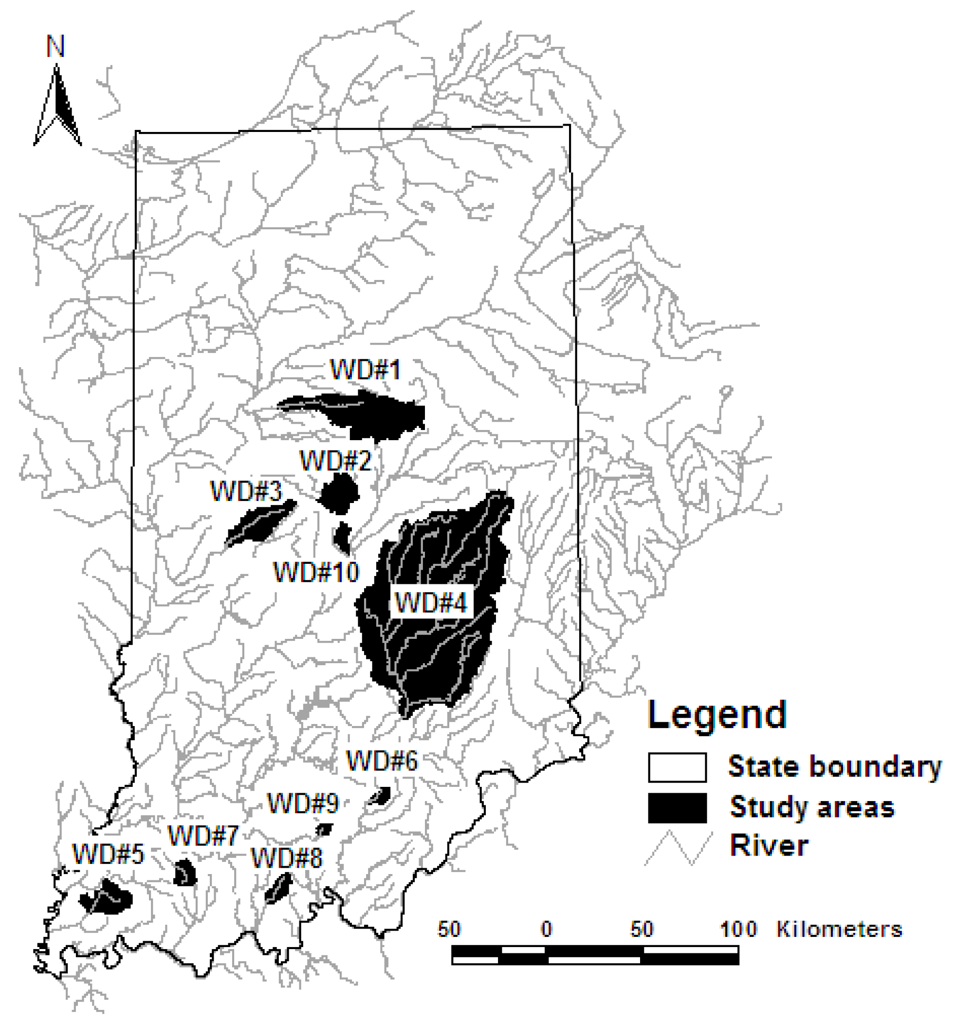
The L-THIA model linked with the two optimization methods was applied to 10 Indiana watersheds to compare optimization performance of the two methods (Figure 6). Brief descriptions for the 10 watersheds are provided in Table 4. The selected watershed areas ranged from 33 to 5811 km2. Five watersheds (WD#1 to WD#5) had crops as the primary land use, and forested area was dominant for watersheds WD#7 to WD#9. WD#6 and WD#10 had pasture/grass and urban as the primary land use, respectively. Major hydrologic soil groups for the study watersheds were B and C.
Figure 6. Study watersheds.
Water 06 03433 g006
The State Soil Geographic (STATSGO) database soil layer was obtained from USEPA [83]. Although the Soil Survey Geographic (SSURGO) database contains higher resolution soil information, the search process and behavior to identify best values when using SSURGO or STATSGO for the two optimization methods are the same. Hydrologic soil group layer was generated by combination of soil layer and hydrologic soil group information for each soil type. Hydrologic soil group was divided in four groups: A for high infiltration, B for moderate infiltration, C for low infiltration, and D for very low infiltration.
The National Land Cover Data (NLCD 2001) for use as the land use layer was obtained from the Multi-Resolution Land Characteristics Consortium web site [84]. The land use type was reclassified into seven categories for L-THIA model application: water, industrial/commercial, row crop, low-density residential, high density residential, grass/pasture, and forest.
The 10 watersheds were selected such that streamflow gage stations operated by U.S. Geological Survey (USGS) were located at the outlets of these watersheds. Streamflow needs to be separated for obtaining direct runoff for the automated calibration process because the CN method estimates direct runoff. The processes of obtaining USGS streamflow data and separating direct runoff were performed using the web-based WHAT program [25] with the digital BFLOW filter method [85].
Table 4. Study area.
WD#NameArea (km2)Land Use (%) *Hydrologic Soil Group (%) **Rainfall Station (COOPID)USGS Station
1Wildcat Creek1024.3I: 1, H: 1, L: 4, O: 7,
C: 80, P: 2, F: 5 W:1
A: 1, B: 52, C: 47, D: 1122638, 122931, 124662, 124667, 128784, 12990503334000
2Eagle Creek268.8I: 0, H: 0, L: 2, O: 8,
C: 73, P: 10, F: 6, W:1
A: 0, B: 50, C: 46, D: 312955703353200
3Big Raccoon Creek364.7I: 0, H: 0, L: 1, O: 5
C: 83, P: 5 F: 7, W: 0
A: 0, B: 49, C: 51, D: 112187303340800
4East Fort White River5844.1I: 0, H: 1, L: 2, O: 6, C: 72, P: 5 F: 13, W:1A: 0, B: 51, C: 47, D: 2121326, 121747, 123527, 123547, 124272, 12464203365500
5Big Creek269.4I: 0, H: 0, L: 1, O: 7,
C: 81, P: 1, F: 9, W: 0
A: 0, B: 54, C: 45 D: 112708303378550
6West Fork Blue River55.7I: 1, H: 0, L: 3, O: 0,
C: 53, P: 0, F: 8, W: 0
A: 0, B: 91, C: 9, D: 012775503302680
7South Fork Patoka River110.7I: 0, H: 0, L: 0, O: 3,
C: 21, P: 6, F: 66, W:3
A: 0, B: 38,C: 57, D: 512844203376350
8Middle Fork Anderson102.8I: 0, H: 0, L: 0, O: 4,
C: 6, P: 17, F: 71, W:1
A: 0, B: 61,C: 36, D: 312772403303300
9Patoka River32.7I: 0, H: 0, L: 0, O: 3,
C: 21, P: 6, F: 66, W:3
A: 0, B: 38,C: 57, D: 512670503374455
10Little Eagle Creek70.1I: 10, H: 20, L: 38, O: 27, C: 0, P: 0, F: 4, W:1A: 0, B: 33,C: 39, D: 2812424903353600
Notes: * I is industrial/commercial; H is high density residential; L is low density residential; O is developed open space; C is crop; P is pasture and grass; F is forest; and W is water; Bold and underline indicates the dominant land use type; ** A means high infiltration (low runoff); B means moderate infiltration(moderate runoff); C means low infiltration (moderate to high runoff); and D means very low infiltration (high runoff); Bold and underlined indicates dominant hydrologic soil group.
The 169 rainfall stations from 562 stations within Indiana operated currently by the National Climatic Data Center (NCDC) were selected, and spatial distribution of rainfall stations as Thiessen polygon GIS data was generated using their location information. NCDC rainfall stations for each watershed are listed in Table 4. Daily precipitation data location information for rainfall stations were obtained from the NCDC website [86]. Periods of 10 years for calibration were selected by considering available rainfall and streamflow data for each watershed.

4. Results

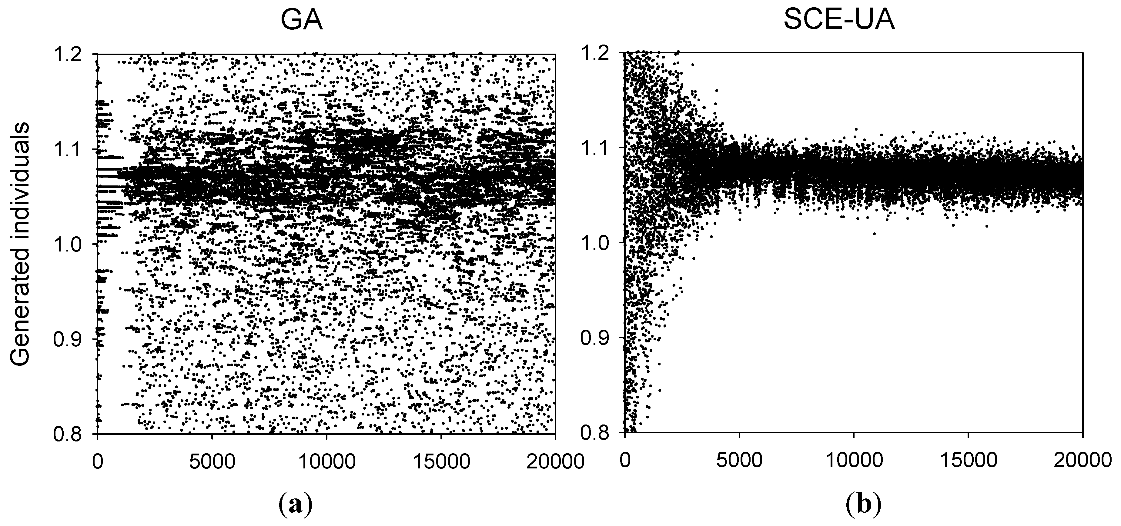
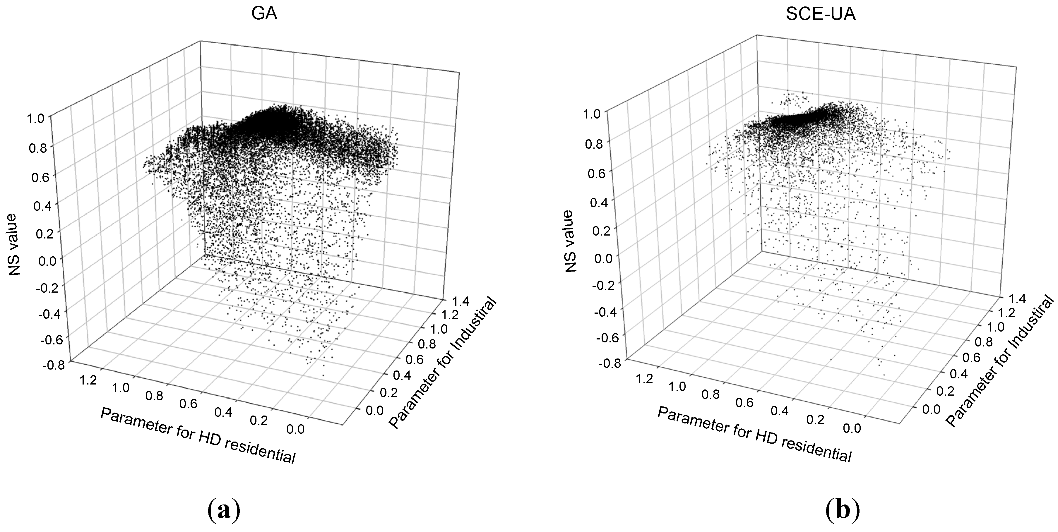
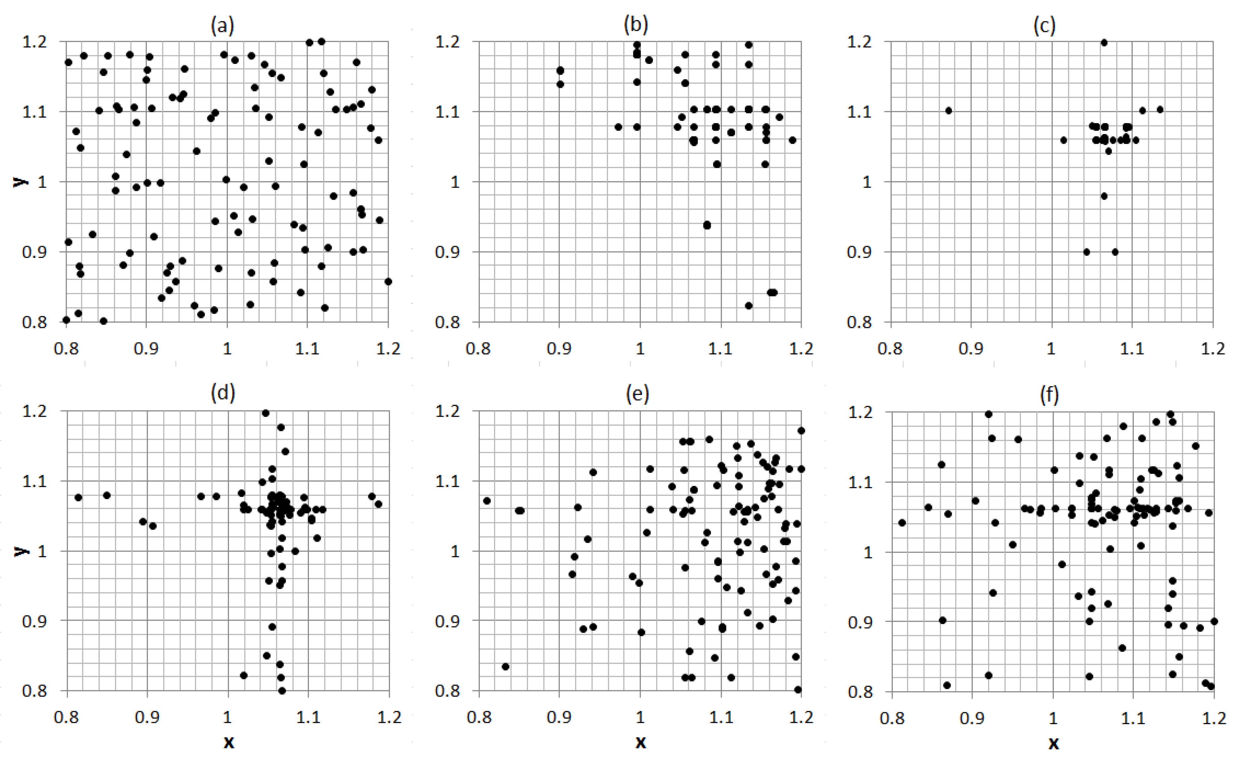
4.1. Generated Individual between GA and SCE-UA

Figure 7 shows the generated individual that was a calibration parameter (PC) to adjust CN values for crop area, which is the dominant land use type (80% of total area) in WD#1. The WD#1 showed the highest NS values, so it was assumed to be a good example for comparing search results between the two methods. Total number of model loop executions was 20,000 for SCE-UA and 20,300 for GA (100 individual per evolution and 200 evolutions). In early stages of evolution, the GA method was very fast and efficiently went to optimal space but after that point, generated individuals were somewhat dispersed compared with the SCE-UA method as shown in Figure 7.
Figure 7. Comparison of generated individuals during evolutionary run between GA and SCE-UA. Number of model runs were 20,000 for SCE-UA and 20,300 (100 individual/generation and 200 generations) for GA. The individual is an optimized parameter of crop land in WD#1 (80% of total area). (a) GA generated individuals; (b) SCE-UA generated individual.
Water 06 03433 g007
The reason the generated individuals are focused on the optimal space until early stages of evolution and then dispersed is well explained by PIKAIA’s user manual [70]. The initial, random population is distributed more or less uniformly in parameter space, but by the 10th evolution, nearly all individuals are concentrated on the central peak. After the 10th evolution, the mutation rate begins to increase. As the mutation rate is further increased, optimized parameters will produce a large horizontal or vertical jump in solution space, named the crosshair pattern. The use of elitism is essential in PIKAIA for improving the best solution. The best solution keeps improving after the 10th evolution, despite the fact that the spatial distribution of the population as a whole exhibits a greater spread about the central peaks in the later phase of the evolutionary run. Figure 8 represents how the GA method generates individuals in each evolution stage. The x and y are individuals for optimized parameters of industrial land use (31% of total area) and high residential area (28% of total area) in WD#10, respectively. Until the 10th evolution, generated individuals are more focused on optimal space as shown in Figure 8c and the crosshair pattern was developed (Figure 8d).
Overall, generated individuals by the SCE-UA were more concentrated in an optimal space compared with those by GA (Figure 7). Figure 9 shows the occurrence frequency of generated individuals for the optimized parameter of cropland (80% of total area) in WD#1. The two optimization methods show the peak in the same range, but frequency at that range for the SCE-UA was about two times higher than that for GA. Figure 7 and Figure 9 illustrate the SCE-UA method focuses more on optimal space for generating individuals.
Figure 8. Evolution of the population during the GA evolutionary run and development of the crosshair pattern on part (D). The x and y are individuals for optimized parameters of industrial land use (31% of total area) and high residential area (28% of total area) in WD#10, respectively. (a) Initial population; (b) 5th generation; (c) 10th generation; (d) 15th generation; (e) 100th generation; (f) 200th generation.
Water 06 03433 g008
Figure 9. Histograms for generated individuals by GA and SCE-UA. Number of model runs were 20,000 for SCE-UA and 20,300 (100 individual/generation and 200 generations) for GA. (a) Histogram for GA; (b) Histogram for SCE-UA.
Water 06 03433 g009

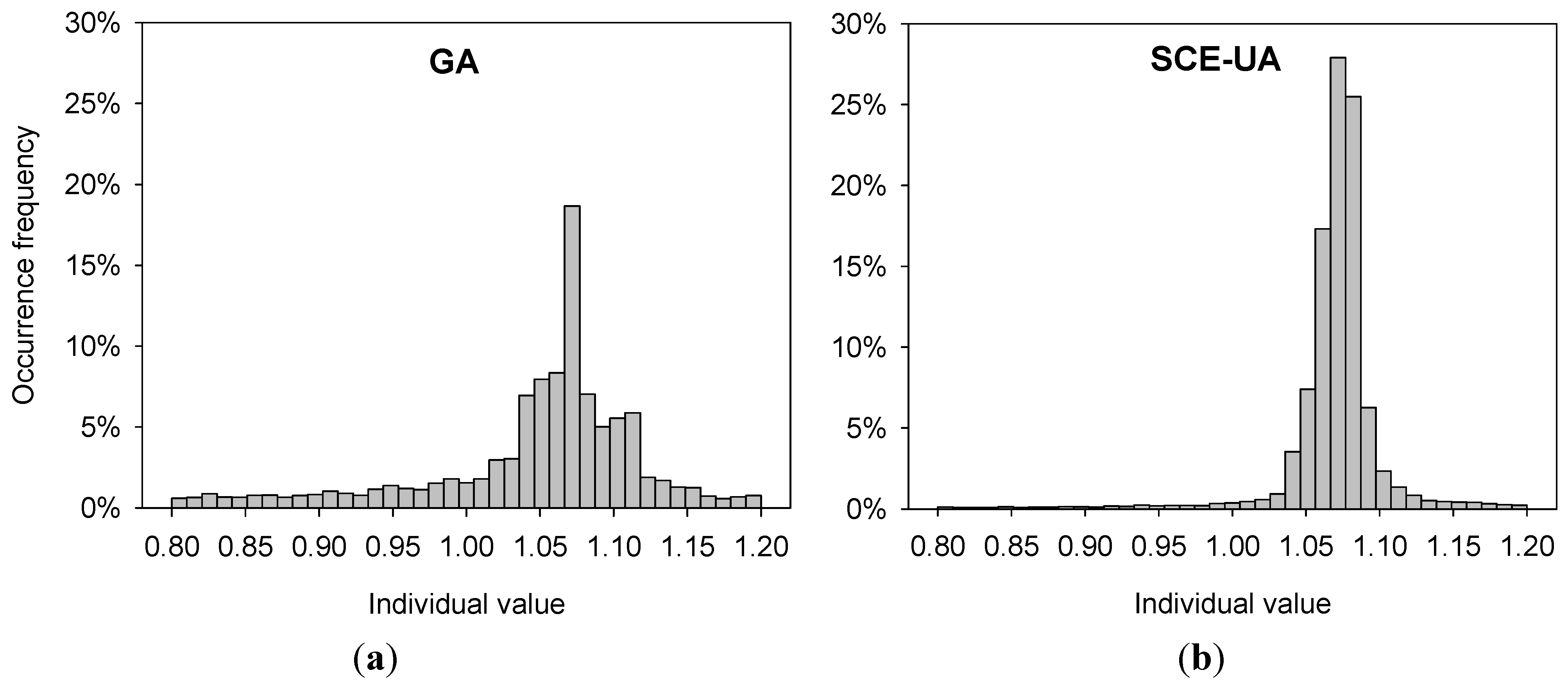
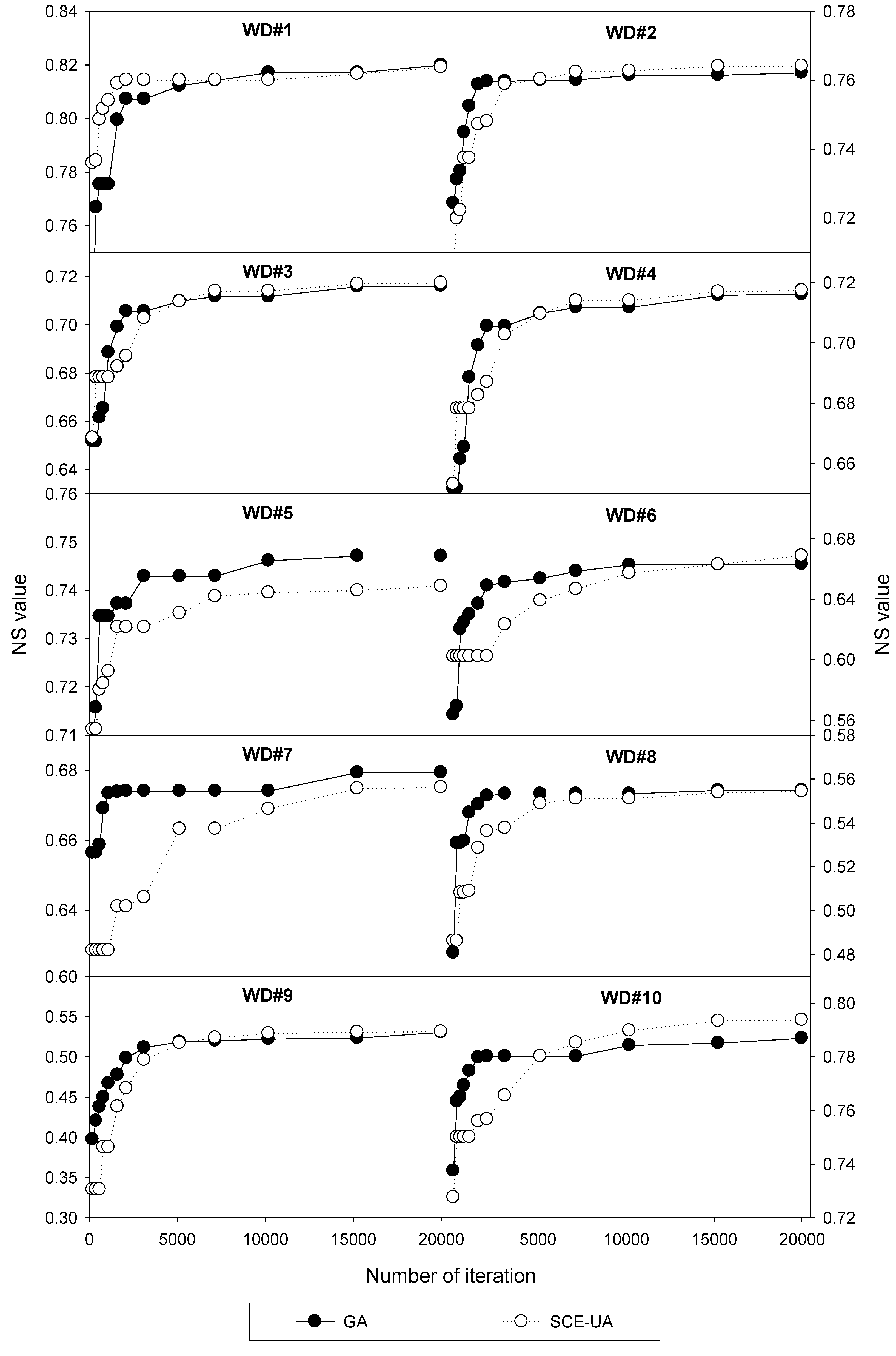
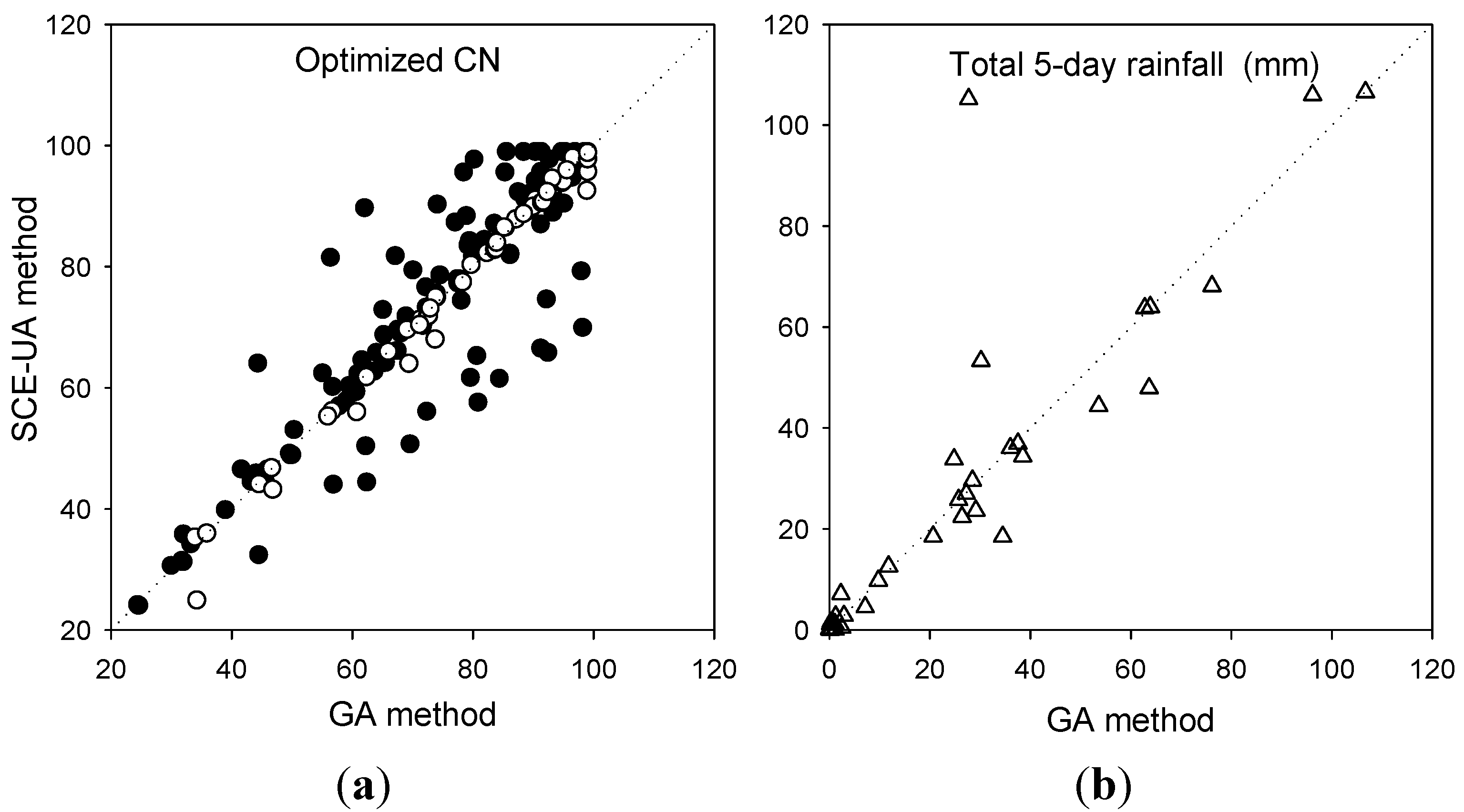
4.2. Performance of GA and SCE-UA for Model Calibration

The generated individuals for SCE-UA fall around a high NS value more often than the generated individuals for GA as shown in Figure 10. The number of model loops executed was 20,000 for SCE-UA and 20,300 (100 individual per generation and 200 generations) for GA. The individuals in x and y were optimized CN multiplication factors for high-density residential and industrial area, respectively.
Figure 10. NS values and individuals for two optimized parameters, which are industrial land use (31% of total area) and high residential area (28% of total area) in WD#10, respectively. Number of model runs were 20,000 for SCE-UA and 20,300 (100 individual/generation and 200 generations) for GA. (a) NS values for GA; (b) NS values for SCE-UA.
Water 06 03433 g010
Total number of model loop executions for automatic calibration with GA or the SCE-UA method for model calibration impacted the results. Until 5150 model loop executions, the GA method showed better performance in L-THIA calibration than the SCE-UA method, and after 5150 times, SCE-UA was better than GA (Table 5).
The performance of GA and SCE-UA linked to L-THIA shows the two global optimizations were able to optimize CN monthly runoff well with most watersheds achieving NS values above 0.5 for 10 year calibration periods (Table 5 and Figure 11). The NS values for calibration ranged from 0.531 to 0.819 for GA and from 0.531 to 0.820 for the SCE-UA method.
Table 5. Automatic calibration performance of L-THIA based on monthly simulation.
WD#Calibration
Period (year)5150 Model Runs20,000 Model Runs
GASCE-UAGASCE-UA
l100.8140.8120.8190.820
2100.7600.7600.7620.764
3100.7100.7100.7160.717
4100.7100.7100.7160.717
5100.7430.7350.7470.741
6100.6540.6390.6630.669
760.6740.6630.6790.675
8100.5530.5490.5550.554
9100.5190.5170.5310.531
10100.7800.7800.7870.794
The filled circles and unfilled circles in Figure 12a show the 1:1 scatter plot of the calibrated CN values for all land uses and for the dominant land use, respectively, found in each watershed. The unfilled circles were more concentrated around the 1:1 line. However, the calibrated CN values for minor land uses in each watershed were unlikely to be as sensitive to calibration as the dominant land uses because they do not significantly influence calculation of the objective functions. Therefore, some filled circles are not as well centered on the 1:1 line. Jeon et al. [45] proposed a global calibration method which obtains one CN parameter set for the best fit to several calibration watersheds rather than an arithmetic average of CN parameters for each calibration watershed to regionalize CN parameters, because unrealistic CN parameters from minor land uses and hydrologic soil groups and realistic CN parameters from major land uses and hydrologic soil groups could provide results that equally regionalize CN values. Figure 12b shows the 1:1 scatter plot for optimized total 5-day rainfall for AMC adjustment, and optimized values fall further from the 1:1 line than CN values.
The parameters identified by SCE-UA for CN values of minor land use type and 5-day rainfall for AMC adjustments were sometimes differently optimized than those for GA as shown in Figure 12. The optimized CN values by SCE-UA for industrial/commercial areas, high and low density residential areas, and total 5-day rainfall were less variable and more concentrated around the average value (Figure 13).
Figure 11. The performance of GA and SCE-UA for model calibration according to the total number of model runs.
Water 06 03433 g011
Figure 12. 1:1 scatter plots of optimized CN and total 5-day rainfall for AMC adjustment. The filled and blank circles represent the calibrated CN values for all land uses and for the dominant land use, respectively, found in each watershed. (a) Optimized CN values; (b) Range of 5-day rainfall for AMC adjustment
Water 06 03433 g012
Figure 13. Comparison of box plots of CN values (a) and total 5-day rainfall (b).
Water 06 03433 g013

5. Discussion

The NS value for the SCE-UA performance was a little higher than that for GA performance when the number of model loop executions by SCE-UA was large enough to search the optimized parameter, and in this study 20,000 times was enough (Figure 9). Cooper et al. [6] evaluated global optimization methods including GA, SCE-UA, and simulated annealing (SA) using a conceptual rainfall runoff model for eleven storms on a Caribbean island, and they also reported that the SCE-UA method provided the best approximations to the optimal solution compared with other methods; for the NS value, the SCE-UA method frequently searches for an exact solution but the GA method searches only near the optimal solution. The SCE-UA method concurrently searches for the optimal value within parameter space using divided complexes as shown in Figure 3. Cooper et al. [6] and Kuczera [11] reported that SCE-UA’s robust capability comes from the periodic global sharing of information among the local simplex searches.
However, the number of model loop executions by the optimization program influenced which global optimization program between GA and SCE-UA was better for automatic calibration of SCS-CN model runoff in this study. The two methods have different ways to search for optimal values. The GA method was faster and efficiently reached the optimal space by the 10th generation, and after the 10th generation, generated individuals were somewhat dispersed to improve the optimization (Figure 6 and Figure 7). Wang et al. [87] found variations in the calibration parameter that were almost same pattern found in this effort and reported in Figure 8 for GA. Table 4 illustrated that GA converges very quickly, and this has been reported by many researchers [88,89,90,91]. Although the SCE-UA method results were somewhat dispersed in initial stages of optimization until around 5000 model executions compared to the GA method, after that point the generated individuals were more focused on the optimal space than those by the GA method (Figure 7, Figure 8, Figure 9). The differences in searching optimal space between GA and SCE-UA methods influenced the optimization performance between the two methods based on the total number of model loop executions (Table 5 and Figure 11).
L-THIA takes a relatively short time to be automatically calibrated when linked with GA or SCE-UA. Total automatic calibration time for WD#4, which is the largest watershed (5844.1 km2) in this study, took 83 min (4980 s) for 20,000 model runs for SCE-UA and 84 min (5040 s) for 20,300 model runs for GA on a Windows XP machine with Intel® Core2 Quad CPU 2.40 GHz and 3.25 GB RAM. In most cases the L-THIA user can select the best optimization method, which is SCE-UA in this study, since the time for calibration is relatively short.
The characteristics of the two algorithms examined in this study might be extended to other models when the most sensitive parameters to the model results are selected as an optimized parameter. The execution of more complex and data intensive hydrological models need significant execution times, so calibrating the complex model becomes an important problem when applying the model on large watershed with long time calibration periods [92]. The number of calibration loop executions with SWAT is very critical so use of an optimization method that is more efficient with fewer calibration loop executions may be required for automatic calibration.
Most researchers emphasized SCE-UA was better than GA when applied to conceptual rainfall-runoff models, which are relatively simple and require short times to run [6,8,10,11]. Van Griensven and Bauwens [93] developed ESWAT, which is SWAT linked with SCE-UA and applied to the Dender River (1384 km2). ESWAT was ended after 8000 runs. If it takes 10 min for a SWAT run, calibration by ESWAT would take 55 days for 8000 runs in this application.
Therefore, a modeler must sometimes select either the GA or SCE-UA method for model calibration considering the available time for calibration. If a model takes a long time to run and the modeler doesn’t have enough time for an optimization program to identify the best values, the GA method is recommended. Otherwise, if the modeler has sufficient time for the optimization approaches to run fully, the SCE-UA method is recommended for more accurate model calibration. In this study, NS value was used as the objective function because it has been widely used for hydrologic model calibration, although NS value has a bias of large stream flow events [94]. The performance of the two optimization methods with other criteria used in objective functions, such as relatively error or root mean square error, should be evaluated in future studies.

6. Conclusions

In this study, the performance of the GA and SCE-UA optimization methods was linked to the L-THIA model, which employs CN and EMC techniques to estimate watershed runoff and nonpoint source pollutant loads, and optimization performances were compared and evaluated through application to 10 watersheds with a 10-year calibration period. The CN values and total five-day rainfall for AMC adjustment were calibrated automatically. The generated individuals by the SCE-UA method were more focused on optimal values as they evolved. The generated individuals by the GA method were generated toward optimal space until the 10th evolution, but after the 10th evolution they were dispersed because mutation rates are increased and a crosshair pattern appeared. Increasing the mutation rate is essential for GA with PIKAIA version to improve the search for the solution.
The two global optimization methods demonstrated acceptable performance for CN runoff simulation, and the calibrated direct runoff values were well matched with observed monthly runoff data. Significant performance differences between the GA and SCE-UA methods for calibration were not found, but the NS values for the SCE-UA are slightly higher than those for the GA method. However, the number of model loop executions for optimization influences the optimization performance between the two methods because the approach to searching optimal space is different. The GA method is recommended when the number of model loop executions for optimization is limited, otherwise SCE-UA’s search method, which globally shares the information from each local simplex search, provided slightly better performance. The results provide important information to help model users select an algorithm for optimization of model parameters and to help developers improve algorithms.

Author Contributions

Ji-Hong Jeon wrote the paper and applied L-THIA linked with GA and SCE-UA; Chan-Gi Park reviewed the references and provided some useful comments; and Bernard A. Engel designed and directed this research.

Conflicts of Interest

The authors declare no conflict of interest.

References

  1. Holland, J.H. Adaptation in Natural and Artificial System; University of Michigan Press: Ann Arbor, MI, USA, 1975. [Google Scholar]
  2. Duan, Q.; Sorooshian, S.; Gupta, V.K. Effective and efficient global optimization for conceptual rainfall-runoff models. Water Resour. Res. 1992, 28, 1015–1031. [Google Scholar] [CrossRef]
  3. Nelder, J.A.; Mead, R. A simplex method for function minimization. Comput. J. 1965, 7, 308–313. [Google Scholar] [CrossRef]
  4. Hooke, R.; Jeeves, T.A. Direct search solutions of numerical and statistical problems. J. ACM 1961, 8, 212–229. [Google Scholar] [CrossRef]
  5. Rosenbrock, H.H. An automatic method for finding the greatest or least value of a function. Comput. J. 1960, 3, 175–184. [Google Scholar] [CrossRef]
  6. Cooper, V.A.; Nguyen, V.T.V.; Nicell, J.A. Evaluation of global optimization methods for conceptual rainfall-runoff model calibration. Water Sci. Technol. 1997, 36, 53–60. [Google Scholar] [CrossRef]
  7. Duan, Q.; Gupta, V.K.; Sorooshian, S. A shuffled complex evolution approach for effective and efficient global minimization. J. Optimiz. Theory Appl. 1993, 76, 501–521. [Google Scholar] [CrossRef]
  8. Franchini, M.; Galeati, G.; Berra, S. Global optimization techniques for the calibration of conceptual rainfall-runoff models. Hydrol. Sci. J. 1998, 43, 443–458. [Google Scholar] [CrossRef]
  9. Gan, T.Y.; Biftu, G.F. Automatic calibration of conceptual rainfall-runoff model: Optimization algorithms, catchment conditions and model structure. Water Resour. Res. 1996, 32, 3513–3524. [Google Scholar] [CrossRef]
  10. Thyer, M.; Kuczera, G.; Bates, B.C. Probabilistic optimization for conceptual rainfall-runoff models: a comparison of the shuffled complex evolution and simulated annealing algorithms. Water Resour. Res. 1999, 35, 767–773. [Google Scholar] [CrossRef]
  11. Kuczera, G. Efficient subspace probabilistic parameter optimization for catchment models. Water Resour. Res. 1997, 33, 177–185. [Google Scholar] [CrossRef]
  12. Vasques, J.A.; Mailer, H.R.; Lence, B.J.; Tolson, B.A.; Foschi, R.O. Achieving water quality system reliability using genetic algorithms. J. Environ. Eng. 2000, 126, 954–962. [Google Scholar] [CrossRef]
  13. Ngo, L.L.; Madsen, H.; Rosbjerg, D. Simulation and optimization modelling approach for operation of the Hoa Binh reservoir, Vietnam. J. Hydrol. 2007, 336, 269–281. [Google Scholar] [CrossRef]
  14. Kerachian, R.; Karamouz, M. A stochastic conflict resolution model for water quality management in reservoir-river systems. Adv. Water Resour. 2007, 30, 866–882. [Google Scholar] [CrossRef]
  15. Park, S.Y.; Choi, J.H.; Wang, S.; Park, S.S. Design of a water quality monitoring network in a large river system using the genetic algorithm. Ecol. Model. 2006, 199, 289–297. [Google Scholar] [CrossRef]
  16. Arsenault, R.; Poulin, A.; Côté, P.; Brissette, F. A comparison of stochastic optimization algorithms in hydrological model calibration. J. Hydrol. Eng. 2013, 19, 1374–1384. [Google Scholar] [CrossRef]
  17. Tolson, B.A.; Shoemaker, C.A. Dynamically dimensioned search algorithm for computationally efficient watershed model calibration. Water Resour. Res. 2007, 43. [Google Scholar] [CrossRef]
  18. Dumedah, G.; Berg, A.A.; Wineberg, M.; Collier, R. Selecting model parameter sets from a trade-off surface generated from the non-dominated sorting genetic algorithm-II. Water Resour. Manag. 2010, 24, 4469–4489. [Google Scholar] [CrossRef]
  19. Wang, W.C.; Cheng, C.T.; Chau, K.W.; Xu, D.M. Calibration of Xinanjiang model parameters using hybrid genetic algorithm based fuzzy optimal model. J. Hydroinform. 2012, 14, 784–799. [Google Scholar] [CrossRef]
  20. Wu, S.J.; Lien, H.C.; Chang, C.H. Calibration of a conceptual rainfall-runoff model using a genetic algorithm integrated with runoff estimation sensitivity to parameters. J. Hydroinform. 2012, 14, 497–511. [Google Scholar] [CrossRef]
  21. Zhang, X.; Srinivasan, R.; Liew, M.V. On the use of multi-algorithm, genetically adaptive multi-objective method for multi-site calibration of the SWAT model. Hydrol. Process. 2010, 24, 955–969. [Google Scholar] [CrossRef]
  22. Zhang, X.; Srinivasan, R.; Arnold, J.; CesarIzaurralde, R.; Bosch, D. Simultaneous calibration of surface flow and base flow simulations: A revisit of the SWAT model calibration framework. Hydrol. Process. 2011, 25, 2313–2320. [Google Scholar] [CrossRef]
  23. Haddadchi, A.; Ryder, D.S.; Evrard, O.; Olley, J. Sediment fingerprinting in fluvial systems: Review of tracers, sediment sources and mixing models. Int. J. Sediment Res. 2013, 28, 560–578. [Google Scholar] [CrossRef]
  24. Rahman, K.; Maringanti, C.; Beniston, M.; Widmer, F.; Abbaspour, K.; Lehmann, A. Streamflow modeling in a highly managed mountainous glacier watershed using SWAT: The Upper Rhone River watershed case in Switzerland. Water Resour. Manag. 2013, 27, 323–339. [Google Scholar] [CrossRef]
  25. Lim, K.J.; Park, Y.S.; Kim, J.; Shin, Y.C.; Kim, N.W.; Kim, S.J.; Jeon, J.-H.; Engel, B.A. Development of genetic algorithm-based optimization module in WHAT system for hydrograph analysis and model application. Comput. Geosci. 2010, 36, 936–944. [Google Scholar] [CrossRef]
  26. Barnhart, B.; Whittaker, G.; Ficklin, D. Improved stream temperature simulation in SWAT using NSGA-II for automatic multi-site calibration. Transactions 2014, 52, 517–530. [Google Scholar]
  27. Kaini, P.; Artita, K.; Nicklow, J.W. Optimizing structural best management practices using SWAT and genetic algorithm to improve water quality goals. Water Resour. Manag. 2012, 26, 1827–1845. [Google Scholar] [CrossRef]
  28. Ahmadi, M.; Arabi, M.; Hoag, D.L.; Engel, B.A. A mixed discrete‐continuous variable multiobjective genetic algorithm for targeted implementation of nonpoint source pollution control practices. Water Resour. Manag. 2013, 49, 8344–8356. [Google Scholar] [CrossRef]
  29. Cao, K.; Huang, B.; Wang, S.; Lin, H. Sustainable land use optimization using Boundary-based Fast Genetic Algorithm. Comput. Environ. Urban 2012, 36, 257–269. [Google Scholar] [CrossRef]
  30. Rodriguez, H.G.; Popp, J.; Maringanti, C.; Chaubey, I. Selection and placement of best management practices used to reduce water quality degradation in Lincoln Lake watershed. Water Resour. Res. 2011, 47. [Google Scholar] [CrossRef]
  31. Limbrunner, J.F.; Vogel, R.M.; Chapra, S.C.; Kirshen, P.H. Classic optimization techniques applied to stormwater and nonpoint source pollution management at the watershed scale. J. Water Res. Plan. Manag. 2013, 139, 486–491. [Google Scholar] [CrossRef]
  32. Lee, J.G.; Selvakumar, A.; Alvi, K.; Riverson, J.; Zhen, J.X.; Shoemaker, L.; Lai, F.H. A watershed-scale design optimization model for stormwater best management practices. Environ. Model. Softw. 2012, 37, 6–18. [Google Scholar] [CrossRef]
  33. Chichakly, K.J.; Bowden, W.B.; Eppstein, M.J. Minimization of cost, sediment load, and sensitivity to climate change in a watershed management application. Environ. Model. Softw. 2013, 50, 158–168. [Google Scholar] [CrossRef]
  34. Artita, K.S.; Kaini, P.; Nicklow, J.W. Examining the possibilities: Generating alternative watershed-scale BMP designs with evolutionary algorithms. Water Resour. Manag. 2013, 27, 3849–3863. [Google Scholar] [CrossRef]
  35. Babbar-Sebens, M.; Barr, R.C.; Tedesco, L.P.; Anderson, M. Spatial identification and optimization of upland wetlands in agricultural watersheds. Ecol. Eng. 2013, 52, 130–142. [Google Scholar] [CrossRef]
  36. Hakimi-Asiabar, M.; Ghodsypour, S.H.; Kerachian, R. Deriving operating policies for multi-objective reservoir systems: Application of self-learning genetic algorithm. Appl. Soft Comput. 2010, 10, 1151–1163. [Google Scholar] [CrossRef]
  37. Yazdi, J.; Salehi Neyshabouri, S.A.A.; Niksokhan, M.H.; Sheshangosht, S.; Elmi, M. Optimal prioritisation of watershed management measures for flood risk mitigation on a watershed scale. J. Flood Risk Manag. 2013, 6, 372–384. [Google Scholar] [CrossRef]
  38. Chen, L.; Kao, S.J.; Traore, S. Predicting and managing reservoir total phosphorus by using modified grammatical evolution coupled with a macro-genetic algorithm. Environ. Model. Softw. 2012, 38, 89–100. [Google Scholar] [CrossRef]
  39. Chenari, K.S.; Ghaderi, M.; Reza, K.M. Improved adaptive genetic algorithm and its application in short-term optimal operation of water resources system. Res. J. Agric. Environ. Manag. 2014, 3, 209–217. [Google Scholar]
  40. Beskowa, S.; Melloc, C.R.; Nortond, L.D.; da Silvac, A.M. Performance of a distributed semi-conceptual hydrological model under tropical watershed conditions. CATENA 2011, 86, 160–171. [Google Scholar] [CrossRef]
  41. Khakbaz, B.; Imam, B.; Hsu, K.; Sorooshian, S. From lumped to distributed via semi-distributed: Calibration strategies for semi-distributed hydrologic models. J. Hydrol. 2012, 418, 61–77. [Google Scholar] [CrossRef]
  42. Chen, J.; Brissette, F.P.; Poulin, A.; Leconte, R. Overall uncertainty study of the hydrological impacts of climate change for a Canadian watershed. Water Resour. Res. 2011, 47. [Google Scholar] [CrossRef]
  43. Lei, X.; Tian, Y.; Liao, W.; Bai, W.; Jia, Y.W.; Jiang, Y.Z.; Wang, H. Development of an AutoWEP distributed hydrological model and its application to the upstream catchment of the Miyun Reservoir. Comput. Geosci. 2012, 44, 203–213. [Google Scholar] [CrossRef]
  44. Shi, P.; Hou, Y.; Xie, Y.; Chen, C.; Chen, X.; Li, Q.; Qu, S.; Fang, X.; Srinivasan, R. Application of a SWAT model for hydrological modeling in the Xixian watershed, China. J. Hydrol. Eng. 2013, 18, 1522–1529. [Google Scholar] [CrossRef]
  45. Jeon, J.H.; Lim, K.J.; Engel, B.A. Regional calibration of SCS-CN L-THIA model: Application for ungauged basins. Water 2014, 6, 1339–1359. [Google Scholar] [CrossRef]
  46. Xu, H.; Chen, Y.; Zeng, B.; He, J.; Liao, Z. Application of SCE-UA algorithm to parameter optimization of Liuxihe model. Trop. Geogr. 2012, 1, 32–37. [Google Scholar]
  47. Song, X.M.; Zhan, C.S.; Xia, J. Integration of a statistical emulator approach with the SCE-UA method for parameter optimization of a hydrological model. Chin. Sci. Bull. 2012, 57, 3397–3403. [Google Scholar] [CrossRef]
  48. Wu, H.; Chen, B. Evaluating uncertainty estimates in distributed hydrological modeling for the Wenjing River watershed in China by GLUE, SUFI-2, and ParaSol methods. Ecol. Eng. 2014, in press. [Google Scholar]
  49. Rasolomanana, S.D.; Lessard, P.; Vanrolleghem, P.A. Single-objective vs. multi-objective autocalibration in modelling total suspended solids and phosphorus in a small agricultural watershed with SWAT. Water Sci. Technol. 2012, 65, 643–652. [Google Scholar] [CrossRef] [PubMed]
  50. Pradhanang, S.M.; Mukundan, R.; Schneiderman, E.M.; Zion, M.S.; Anandhi, A.; Pierson, D.C.; Frei, A.; Easton, Z.M.; Fuka, D.; Steenhuis, T.S. Streamflow responses to climate change: Analysis of hydrologic indicators in a New York City water supply watershed. J. Am. Water Resour. Assoc. 2013, 49, 1308–1326. [Google Scholar] [CrossRef]
  51. Poulin, A.; Brissette, F.; Leconte, R.; Arsenault, R.; Malo, J.S. Uncertainty of hydrological modelling in climate change impact studies in a Canadian, snow-dominated river basin. J. Hydrol. 2011, 409, 626–636. [Google Scholar] [CrossRef]
  52. Ricard, S.; Bourdillon, R.; Roussel, D.; Turcotte, R. Global calibration of distributed hydrological models for large-scale applications. J. Hydrol. Eng. 2012, 18, 719–721. [Google Scholar] [CrossRef]
  53. Liong, S.Y.; Raghavan, S.V.; Vu, M.T. Climate Change and Its Impacts on Streamflow: WRF and SCE-Optimized SWAT Models. In Data Assimilation for Atmospheric, Oceanic and Hydrologic Applications; Springer Berlin: Heidelberg, Germany, 2013; Volume II, pp. 411–428. [Google Scholar]
  54. Nasonova, O.N.; Gusev, E.M.; Kovalev, E.E. Application of a land surface model for simulating rainfall streamflow hydrograph: 1. Model calibration. Water Resour. 2011, 38, 155–168. [Google Scholar] [CrossRef]
  55. Casimiro, L.; Sven, W.; Labat, D.; Guyot, J.L.; Ardoin-Bardin, S. Assessment of climate change impacts on the hydrology of the Peruvian Amazon-Andes basin. Hydrol. Process. 2011, 25, 3721–3734. [Google Scholar] [CrossRef]
  56. Bao, H.J.; Wang, L.L.; Li, Z.J.; Zhao, L.N.; Zhang, G.P. Hydrological daily rainfall-runoff simulation with BTOPMC model and comparison with Xin’anjiang model. Water Sci. Eng. 2010, 3, 121–131. [Google Scholar]
  57. Kwon, H.; Grunwald, S.; Beck, H.; Jung, Y. Automatic calibration of a hydrologic model for simulating groundwater table fluctuations on farms in the everglades agricultural area of south Florida. Irrig. Drain. 2014, 63, 538–549. [Google Scholar] [CrossRef]
  58. Guo, J.; Zhou, J.; Zou, Q.; Liu, Y.; Song, L. A novel multi-objective shuffled complex differential evolution algorithm with application to hydrological model parameter optimization. Water Resour. Manag. 2013, 27, 2923–2946. [Google Scholar] [CrossRef]
  59. Kang, M.; Park, S. Modeling water flows in a serial irrigation reservoir system considering irrigation return flows and reservoir operations. Agric. Water Manag. 2014, 143, 131–141. [Google Scholar] [CrossRef]
  60. Dong, J.R.; Zheng, C.Y.; Kan, G.Y.; Zhao, M. Optimal scheduling of hydrothermal system with network and ramping via SCE-UA method. Open Cybern. Syst. J. 2013, 7, 55–64. [Google Scholar] [CrossRef]
  61. Kang, T.; Lee, S. Modification of the SCE-UA to include constraints by embedding an adaptive penalty function and application: Application approach. Water Resour. Manag. 2014, 28, 2145–2159. [Google Scholar] [CrossRef]
  62. Dakhlaoui, H.; Bargaoui, Z.; Bárdossy, A. Toward a more efficient calibration schema for HBV rainfall-runoff model. J. Hydrol. 2012, 444, 161–179. [Google Scholar] [CrossRef]
  63. Chu, W.; Gao, X.; Sorooshian, S. Improving the shuffled complex evolution scheme for optimization of complex nonlinear hydrological systems: Application to the calibration of the Sacramento soil‐moisture accounting model. Water Resour. Res. 2010, 46. [Google Scholar] [CrossRef]
  64. Agrawal, R.K.; Singh, J.K. Application of a genetic algorithm in the development and optimization of a non-linear dynamic runoff model. Biosyst. Eng. 2003, 86, 87–95. [Google Scholar] [CrossRef]
  65. Charbonneau, P.; Knapp, B. A User’s Guide to PIKAIA 1.0.; NCAR technical note NCAR/TN-418+IA; High Altitude Observatory National Center for Atmospheric Research: Boulder, CO, USA, 1995. [Google Scholar]
  66. Park, Y.S.; Lim, K.J.; Theller, L.; Engel, B.A. L-THIA GIS Manual (Long-Term Hydrologic Impact Assessment). 2013. Available online: https://engineering.purdue.edu/mapserve/LTHIA7/arclthia/LTHIA2013_Manual.pdf (accessed on 12 July 2014).
  67. L-THIA WEB. Available online: https://engineering.purdue.edu/~lthia/ (accessed on 12 July 2014).
  68. Grove, M.; Harbor, J.; Engel, B.A.; Muthukrishnan, S. Impact of urbanization on surface hydrology, Little Eagle Creek, Indiana, and analysis of L-THIA model sensitivity to data resolution. Phys. Geogr. 2001, 22, 135–153. [Google Scholar]
  69. Kim, Y.; Engel, B.A.; Lim, K.J.; Larson, V.; Duncan, B. Runoff impacts of land-use change in Indian river lagoon watershed. J. Hydrol. Eng. 2002, 7, 245–251. [Google Scholar] [CrossRef]
  70. Choi, J.Y.; Engel, B.A.; Muthukrishnan, S.; Harbor, J. GIS based long term hydrologic impact evaluation for watershed urbanization. J. Am. Water Resour. Assoc. 2003, 39, 623–635. [Google Scholar] [CrossRef]
  71. Gunn, R.; Martin, A.; Engel, B.; Ahiablame, L. Development of two indices for determining hydrologic implications of land use changes in urban areas. Urban Water J. 2012, 9, 239–248. [Google Scholar] [CrossRef]
  72. Bhaduri, B.; Harbor, J.; Engel, B.A.; Grove, M. Assessing watershed-scale, long-term hydrologic impacts of land use change using a GIS-NPS model. J. Environ. Manag. 2000, 26, 643–658. [Google Scholar] [CrossRef]
  73. Zhang, J.; Shen, T.; Liu, M.; Wan, Y.; Liu, J.; Li, J. Research on non-point source pollution spatial distribution of Qingdao based on L-THIA model. Math Comput. Model. 2011, 54, 1151–1159. [Google Scholar] [CrossRef]
  74. You, Y.Y.; Jin, W.B.; Xiong, Q.X.; Xue, L.; Ai, T.C.; Li, B.L. Simulation and validation of non-point source nitrogen and phosphorus loads under different land uses in Sihu Basin, Hubei Province, China. Proc. Environ. Sci. 2012, 13, 1781–1797. [Google Scholar] [CrossRef]
  75. Tang, Z.; Engel, B.A.; Pijanowski, B.C.; Lim, K.L. Forecasting land use change and its environmental impact at a watershed scale. J. Environ. Manag. 2005, 76, 35–45. [Google Scholar] [CrossRef]
  76. Tang, Z.; Engel, B.A.; Lim, K.J.; Pijanowski, B.C. Minimizing the impact of urbanization on long term runoff. J. Am. Water Resour. Assoc. 2005, 41, 1347–1359. [Google Scholar] [CrossRef]
  77. Choi, J.Y.; Engel, B.A.; Harbor, J. GIS and Web-Based DSS for Preliminary TMDL Development. In Total Maximum Daily Load (TMDL) Regulation; American Society of Agricultural and Biological Engineers: St. Joseph, MI, USA, 2002; pp. 477–484. [Google Scholar]
  78. Ahiablame, L.M.; Engel, B.A.; Chaubey, I. Representation and evaluation of low impact development practices with L-THIA-LID: An example for site planning. Environ. Pollut. 2012, 1, 1–13. [Google Scholar] [CrossRef]
  79. Hunter, J.G.; Engel, B.A.; Quansah, J.E. Web-Based Low Impact Development Decision Support Tool for Watershed Planning. In Proceedings of Low Impact Development, San Francisco, CA, USA, 11–14 April 2010; pp. 484–495.
  80. Ahiablame, L.M.; Engel, B.A.; Chaubey, I. Effectiveness of low impact development practices in two urbanized watersheds: Retrofitting with rain barrel/cistern and porous pavement. J. Environ. Manag. 2013, 119, 151–161. [Google Scholar] [CrossRef]
  81. Nash, J.E.; Sutcliffe, J.V. River flow forecasting through conceptual model. Part 1: A discussion of principles. J. Hydrol. 1970, 10, 282–290. [Google Scholar] [CrossRef]
  82. United States Department of Agriculture, Natural Resources Conservation Service (USDA-NRCS). Urban Hydrology for Small Watersheds; Technical Release 55 USDA-NRCS, 210-VI-TR-55; USDA-NRCS: Washington, DC, USA, 1986.
  83. Water: Science & Technology. Available online: http://www.epa.gov/waterscience/ftp/basins/gis_data/huc/ (accessed on 12 July 2014).
  84. Multi-Resolution Land Characteristics Consortium. Available online: http://www.mrlc.gov/index.asp/ (accessed on 12 July 2014).
  85. WHAT: Web-based Hydrograph Analysis Tool. Available online: https://engineering.purdue.edu/~what/ (accessed on 12 July 2014).
  86. National Climatic Data Center (NCDC). Available online: http://www.ncdc.noaa.gov/cdo-web/ (accessed on 12 July 2014).
  87. Wang, K.; Wang, N. A novel RNA genetic algorithm for parameter estimation of dynamic systems. Chem. Eng. Res. Des. 2010, 88, 1485–1493. [Google Scholar] [CrossRef]
  88. Coello, C.A.C.; van Veldhuizen, D.A.; Lamont, G.B. Evolutionary Algorithms for Solving Multi-Objective Problems; Kluwer Academic Publishers: New York, NY, USA, 2002. [Google Scholar]
  89. Deb, K.; Mohan, M.; Mishra, S. A Fast Multi-Objective Evolutionary Algorithm for Finding Well-Spread Pareto-Optimal Solutions; KanGAL Report No. 2003002; Indian Institute of Technology: Kanpur, India, 2003. [Google Scholar]
  90. Reed, P.; Minsker, B.S.; Goldberg, D.E. Simplifying multiobjective optimization: An automated design methodology for the nondominated sorted genetic algorithm-II. Water Resour. Res. 2003, 39. [Google Scholar] [CrossRef]
  91. Tang, Y.; Reed, P.; Wagener, T. How effective and efficient are multiobjective evolutionary algorithms at hydrologic model calibration? Hydrol. Earth Syst. Sci. 2006, 10, 289–307. [Google Scholar] [CrossRef]
  92. Gorgan, D.; Bacu, V.; Mihon, D.; Rodila, D.; Abbaspour, K.; Rouholahnejad, E. Grid based calibration of SWAT hydrological models. Nat. Hazard. Earth Syst. Sci. 2012, 12, 2411–2423. [Google Scholar] [CrossRef]
  93. Van Griensven, A.; Bauwens, W. Multiobjective autocalibration for semidistributed water quality models. Water Resour. Res. 2003, 39. [Google Scholar] [CrossRef]
  94. Willmott, C.J.; Robeson, S.M.; Matsuura, K. A refined index of model performance. Int. J. Climatol. 2012, 32, 2088–2094. [Google Scholar] [CrossRef]

