Do Water Rights Affect Technical Efficiency and Social Disparities of Crop Production in the Mediterranean? The Spanish Ebro Basin Evidence

Abstract
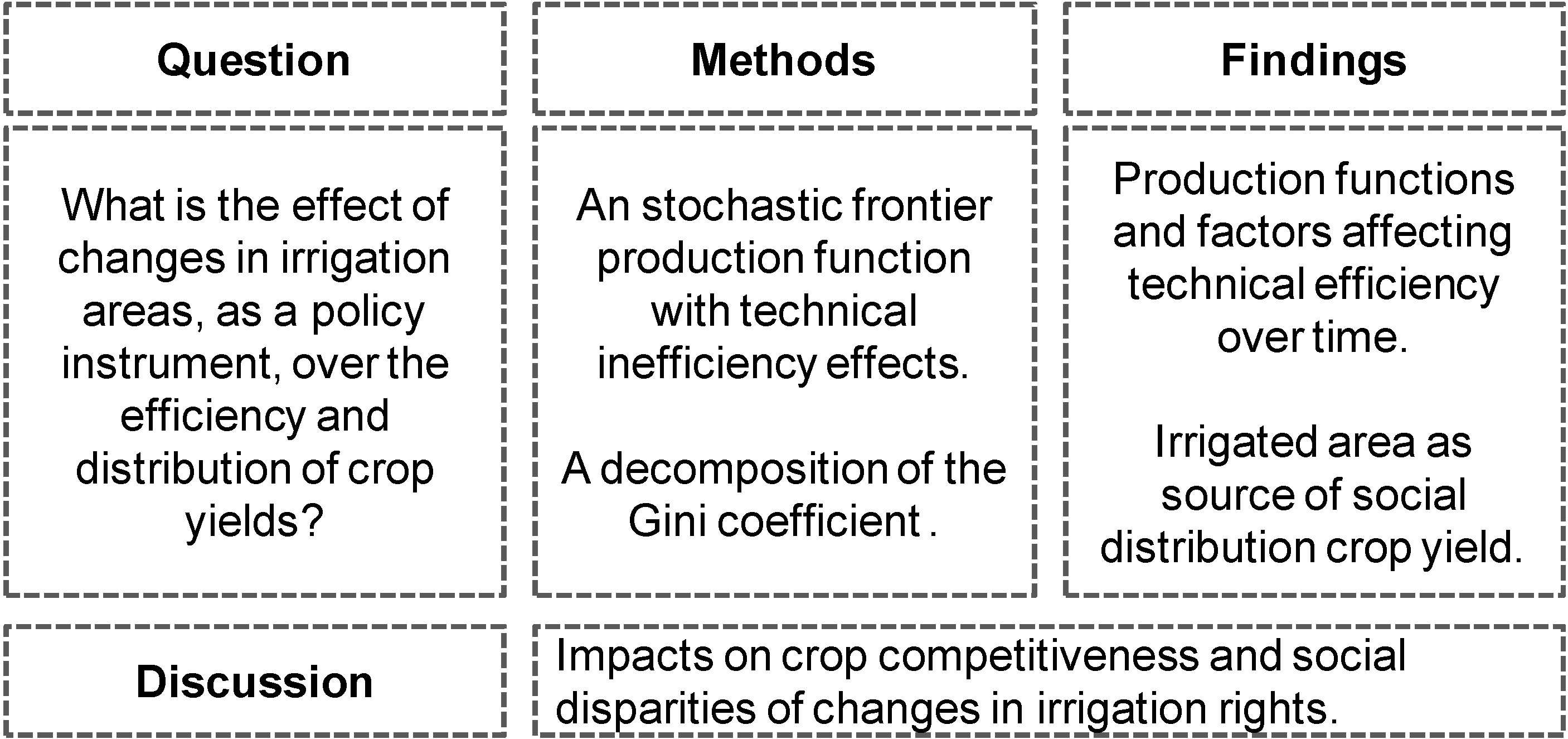
:1. Introduction

2. Methods
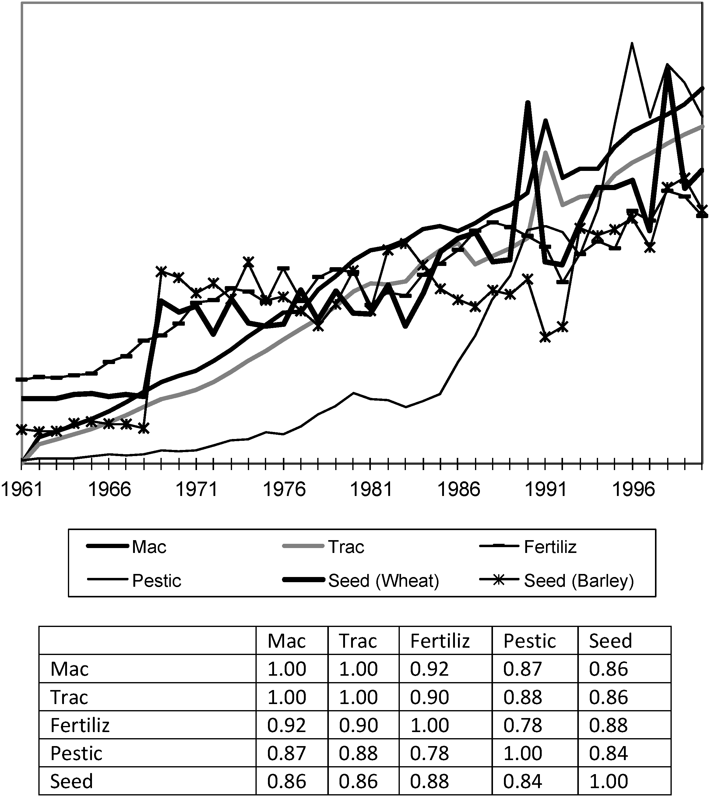
2.1. Data

| Crop | % of the Total Agricultural Area | Dominant Cropping System |
|---|---|---|
| Wheat | 17.0% | Rainfed |
| Barley | 26.4% | Rainfed |
| Maize | 2.2% | Irrigation |
| Alfalfa | 4.4% | Irrigation |
| Grapevine | 4.2% | Rainfed |
| Total | 54.2% |
| Type of Variable | Contribution to the Analysis | Name | Definition | Unit | Source of Data (*) |
|---|---|---|---|---|---|
| Socio-economic factors | Output | Yit | Crop yield at a site in year t | T/ha | MARM |
| Input factor | Techit | Proxi of technological development. Derived from Principal component analysis (PCA) of fertilizers and machinery in year t | Standardized units | Own elaboration from FAOSTAT | |
| Input factor | Lit | Total employment of agricultural sector at a site in year t | 1000 people | LFS; INE | |
| Input factor | Irrigit | Net water needs of crops in year t | mm/month | CHEBRO | |
| Input factor | Irrig_areait | Irrigated area by crop type | Ha | MARM | |
| Efficiency driver | %Irrig_areait | Irrigated area by crop type as proportion of total agricultural area (%) | Ratio | MARM | |
| Efficiency driver | HDIit | Human Development Index at a site in the year t (%) | Index | IVIE; Bancaja | |
| Efficiency driver | MacSharryt | Dummy variable equal to 1 after MacSharry Reform introduction in 1994, 0 before this year | 1 or 0 as a function of the introduction of the reform | Own elaboration | |
| Efficiency driver | Agenda2000t | Dummy variable equal to 1 after Agenda2000 Reform introduction in 2001, 0 before this year | 1 or 0 as a function of the introduction of the reform | Own elaboration | |
| Time trend | t | t = 1 for 1976, t = 27 for 2002. | Year sequence | Own elaboration | |
| Bio-phisical factors | Efficiency driver | Altitudei | Total area in Km2 by altitude zone: 0–600, 601–1000 and more than 1000 m of altitude | Km2 | INE |
| Input factor | Area_ebroi | Dummy variables indicating the 3 main areas of the basin: Northern, Central and Low Ebro | 1 or 0 as a function of the area | Own elaboration | |
| Input factor | Precit | Total precipitation at a site in the year t | mm/year | AEMET | |
| Input factor | T_Meanit | Average temperature at a site in the year t | °C | AEMET | |
| Input factor | Droit | Dummy variable indicating drought year (1 for drought years, 0 in other cases) | 1 or 0 as a function of SPI index | Own elaboration from AEMET |
2.2. Stochastic Frontier Production Function with Technical Inefficiency Effects
2.3. Distributional Efficiency Using the Decomposition of the Gini Coefficient
3. Results
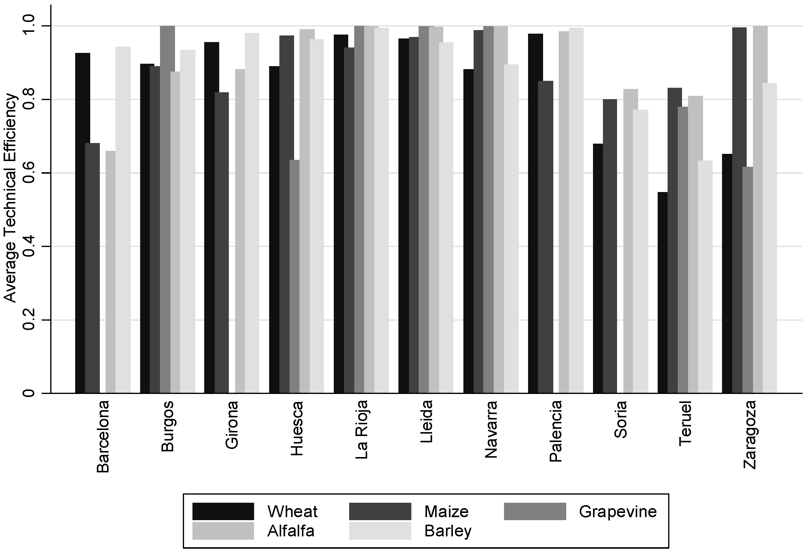
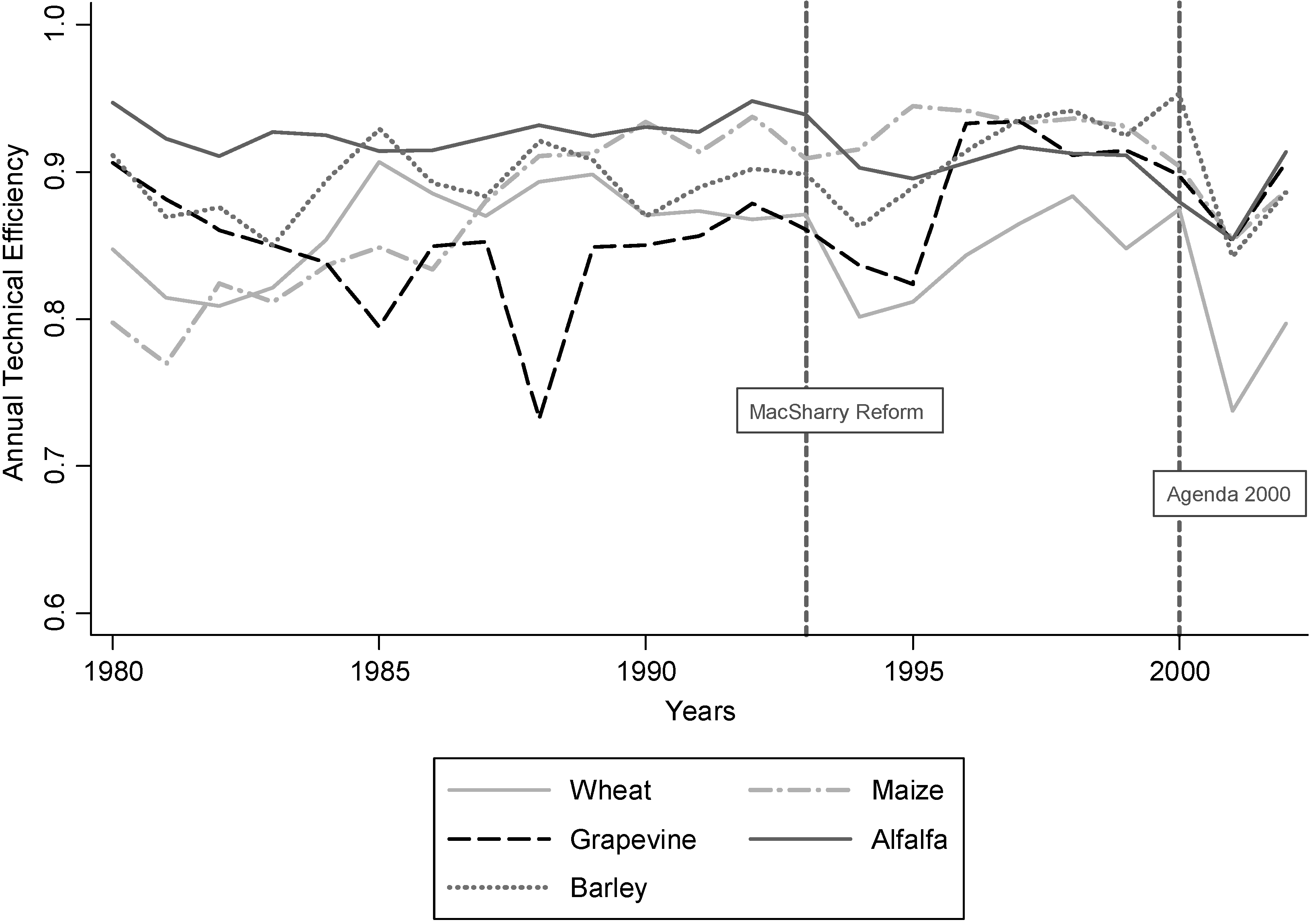
3.1. Production Functions and Factors Affecting Technical Efficiency over Time
| Dependent Variable: ln(Yield) | |||||
|---|---|---|---|---|---|
| Explanatory Variables | Wheat | Maize | Grapevine | Alfalfa | Barley |
| Tech | 0.0818 *** | −0.0327 ** | 0.0058 | 0.0074 | 0.0800 *** |
| [0.022] | [0.014] | [0.026] | [0.012] | [0.021] | |
| ln(L) | 0.1359 * | −0.2176 *** | −0.5492 *** | −0.0713 ** | 0.0835 |
| [0.070] | [0.053] | [0.095] | [0.028] | [0.072] | |
| Cent_Ebro | −0.0931 | −0.1030 ** | −0.3556 *** | −0.0542 | −0.0701 |
| [0.075] | [0.045] | [0.100] | [0.037] | [0.072] | |
| Northern_Ebro | −0.3647 *** | −0.1185 * | −0.7678 *** | −0.1121 ** | −0.3980 *** |
| [0.137] | [0.070] | [0.198] | [0.051] | [0.114] | |
| ln(Irrig) | 0.0488 * | 0.0558 ** | −0.1740 ** | 0.1418 *** | −0.0084 |
| [0.025] | [0.022] | [0.069] | [0.013] | [0.022] | |
| ln(Irrig_area) | −0.0301 | 0.0381 *** | 0.1350 *** | 0.0243 *** | −0.0527 *** |
| [0.023] | [0.012] | [0.020] | [0.008] | [0.020] | |
| ln(Precyear) | 0.1851 *** | 0.0245 | −0.0262 | 0.1374 *** | 0.1072 * |
| [0.065] | [0.041] | [0.078] | [0.032] | [0.062] | |
| ln(T_Meanyear) | −0.8508 ** | −0.1174 | 1.5134 *** | 0.3849 *** | −1.2215 *** |
| [0.371] | [0.188] | [0.439] | [0.130] | [0.279] | |
| Dro | −0.1297 ** | −0.0258 | −0.1471 ** | −0.0195 | −0.2269 *** |
| [0.051] | [0.035] | [0.058] | [0.029] | [0.050] | |
| T | 0.0035 | 0.0198 *** | 0.0098 | 0.0073 ** | −0.0017 |
| [0.007] | [0.005] | [0.008] | [0.004] | [0.007] | |
| Constant | 1.5550 | 1.9793 *** | −0.5115 | 0.7496 | 3.6684 *** |
| [1.416] | [0.604] | [1.120] | [0.456] | [1.022] | |
| Observations: | 276 | 239 | 164 | 306 | 265 |
| Technical Inefficiency = U | |||||
|---|---|---|---|---|---|
| Explanatory Variables | Wheat | Maize | Grapevine | Alfalfa | Barley |
| Altitude(0–600) | 0.0007 *** | −0.0006 ** | 0.0031 | 0.0003 | 0.0007 *** |
| [0.000] | [0.000] | [0.002] | [0.000] | [0.000] | |
| Altitude(601–1000) | 0.0001 | −0.0002 | −0.0024 * | −0.0000 | −0.0000 |
| [0.000] | [0.000] | [0.001] | [0.000] | [0.000] | |
| Altitude(+1000) | 0.0007 *** | 0.0002 ** | 0.0023 | 0.0013 *** | 0.0008 *** |
| [0.000] | [0.000] | [0.002] | [0.000] | [0.000] | |
| %Irrig_area | −0.1226 * | −0.0557 *** | −0.1471 *** | −0.1761 *** | −0.3870 * |
| [0.066] | [0.014] | [0.053] | [0.044] | [0.233] | |
| HDI | 0.3600 | −0.8561 *** | 0.5497 | −0.2694 | 0.6372 * |
| [0.276] | [0.324] | [0.640] | [0.283] | [0.377] | |
| MacSharry | 1.1563 * | −0.1879 | 0.4204 | 1.2207 | 0.7645 |
| [0.666] | [0.766] | [1.027] | [0.751] | [0.922] | |
| Agenda2000 | 1.7112 ** | 2.1257 ** | 0.9079 | 0.6947 | 2.3135 ** |
| [0.684] | [0.930] | [0.993] | [0.726] | [0.959] | |
| t | −0.2697 * | 0.2519 * | −0.1977 | −0.0061 | −0.3585 ** |
| [0.141] | [0.144] | [0.315] | [0.141] | [0.178] | |
| Constant | −36.7713 | 76.0302 *** | −69.3678 | 22.3471 | −60.6567 * |
| [23.993] | [28.069] | [52.776] | [24.382] | [33.044] | |
| Observations | 276 | 239 | 164 | 306 | 265 |
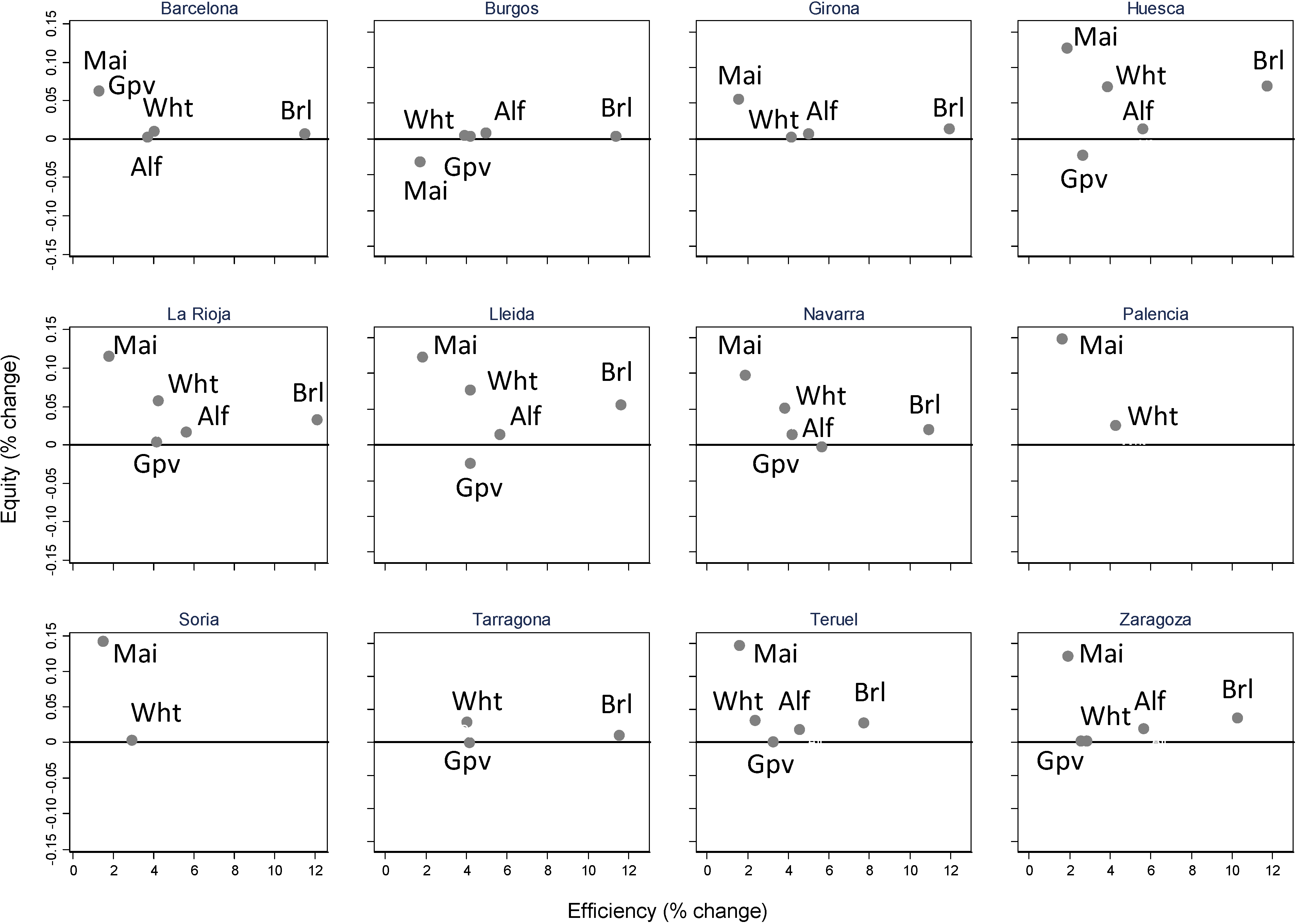
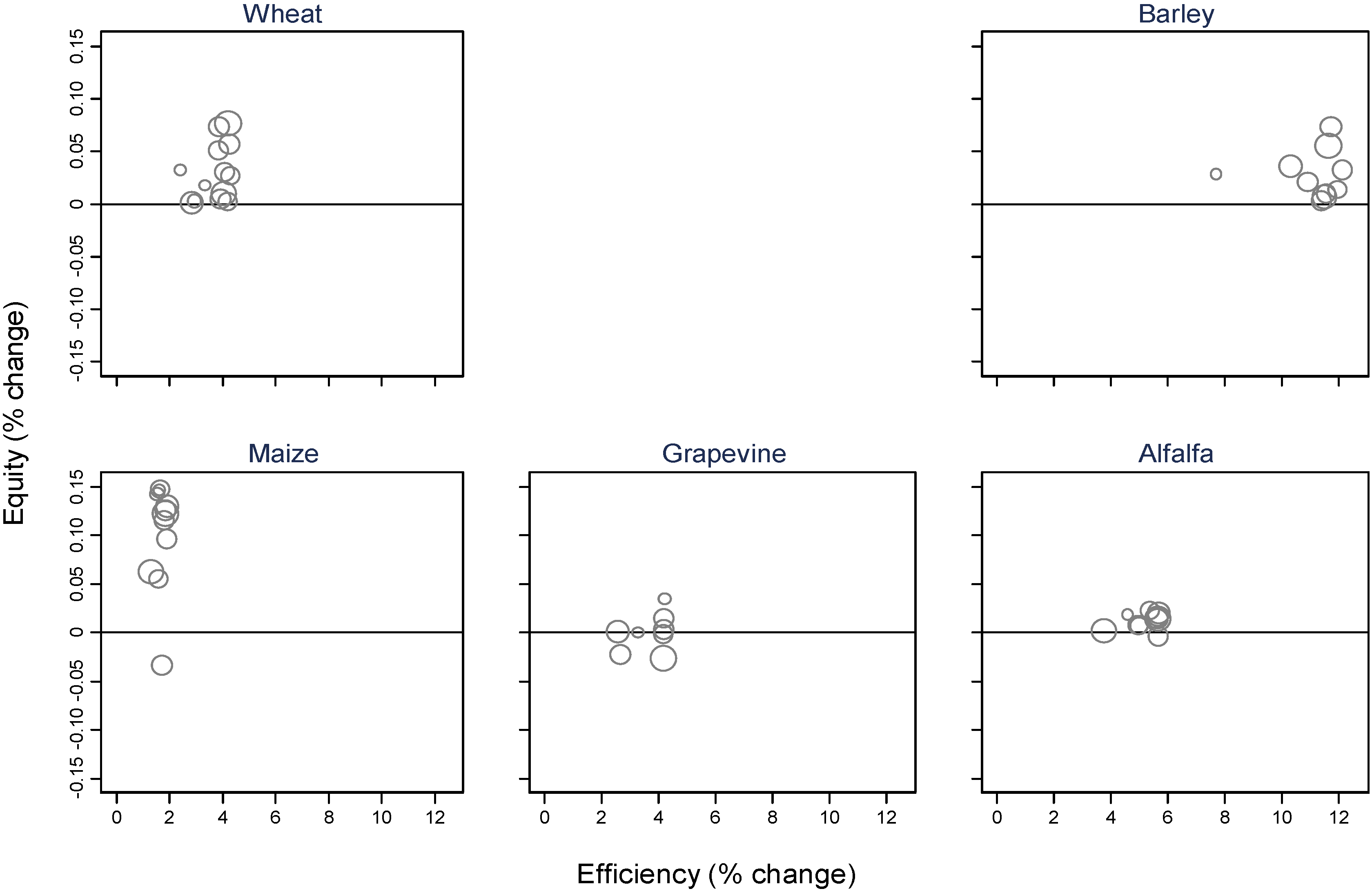
3.2. Crop Yield Sources and Their Impact on Social Distribution
| Crop | G | Sk = Irrigated area | Gk = Irrigated area | Rk = Irrigated area | % Change | [95% Conf. Interval] |
|---|---|---|---|---|---|---|
| Wheat | 0.22 | 0.05 | 0.57 | 0.25 | −0.0166 | [−0.0320 to −0.0066] |
| Maize | 0.22 | 0.12 | 0.20 | 0.79 | −0.0372 | [−0.0491 to −0.0256] |
| Barley | 0.18 | 0.03 | 0.46 | 0.10 | −0.0192 | [−0.0241 to −0.0136] |
| Alfalfa | 0.16 | 0.01 | 0.28 | 0.62 | 0.0016 | [−0.0004 to 0.0036] |
| Grapevine | 0.32 | 0.02 | 0.66 | 0.41 | −0.0032 | [−0.0109 to 0.0013] |
3.3. Water Policy Implications on Technical Efficiency and Social Equity

4. Discussion and Policy Implications
5. Conclusions
Acknowledgments
Author Contributions
Conflicts of Interest
References
- Gaál, M.; Quiroga, S.; Fernandez-Haddad, Z. Potential impacts of climate change on agricultural land use suitability of the Hungarian counties. Reg. Environ. Chang. 2014, 14, 597–610. [Google Scholar] [CrossRef]
- González-Zeas, D.; Quiroga, S.; Iglesias, A.; Garrote, L. Looking beyond the average agricultural impacts in defining adaptation needs in Europe. Reg. Environ. Chang. 2014, 14, 1983–1993. [Google Scholar] [CrossRef]
- Organisation for Economic Co-operation and Development (OECD). Sustainable Management of Water Resources in Agriculture; OECD: Paris, France, 2010. [Google Scholar]
- Bruns, B.; Meinzen-Dick, R.S. Negotiating Water Rights; International Food Policy Research Institute-Consultative Group on International Agricultural Research (IFPRI-CGIAR), Intermediate Technology Publications: Washington, DC, USA, 2000. [Google Scholar]
- Food and Agriculture Organization of the United Nations (FAO). Crops and Drops: Making the Best Use of Water for Agriculture; FAO: Rome, Italy, 2002. [Google Scholar]
- Gómez-Limón, J.A.; Arriaza, M.; Berbel, J. Conflicting implementation of agricultural and water policies in irrigated areas in the EU. J. Agric. Econ. 2002, 53, 259–281. [Google Scholar] [CrossRef]
- Iglesias, A.; Garrote, L.; Quiroga, S.; Moneo, M. A regional comparison of the effects of climate change on agriculture in Europe. Clim. Chang. 2012, 112, 29–46. [Google Scholar] [CrossRef]
- Quiroga, S.; Fernández-Haddad, Z.; Iglesias, A. Crop yields response to water pressures in the Ebro basin in spain: Risk and water policy implications. Hydrol. Earth Syst. Sci. 2011, 15, 505–518. [Google Scholar] [CrossRef] [Green Version]
- Quiroga, S.; Garrote, L.; Iglesias, A.; Fernández-Haddad, Z.; Schlickenrieder, J.; de Lama, B.; Mosso, C.; Sanchez-Arcilla, A. The economic value of drought information for water management under climate change: A case study in the Ebro Basin. Nat. Hazard. Earth Syst. Sci. 2011, 11, 1–15. [Google Scholar] [CrossRef]
- Manos, B.; Bournaris, T.; Kamruzzaman, M.; Begum, A.A.; Papathanasiou, J. Regional impact of irrigation water pricing in Greece under alternative scenarios of European policy: A multicriteria analysis. Reg. Stud. 2006, 40, 1055–1068. [Google Scholar] [CrossRef]
- Liu, J.; Wiberg, D.; Zehnder, A.J.B.; Yang, H. Modeling the role of irrigation in winter wheat yield, crop water productivity, and production in China. Irrig. Sci. 2007, 26, 21–33. [Google Scholar] [CrossRef]
- Pender, J.; Gebremedhin, B. Land Management, Crop Production, and Household Income in the Highlands of Tigray, Northern Ethiopia: An Econometric Analysis. In Strategies for Sustainable Land Management in the East African Highlands; Pender, J., Place, F., Ehui, S.K., Eds.; International Food Policy Research Institute (IFPRI): Washington, DC, USA, 2006; pp. 107–139. [Google Scholar]
- Bournaris, T.; Manos, B. European union agricultural policy scenarios’ impacts on social sustainability of agricultural holdings. Int. J. Sustain. Dev. World 2012, 19, 426–432. [Google Scholar] [CrossRef]
- Atwi, M.; Arrojo, P. Local Government Practices and Experiences in IWRM in the River Basin of the Ebro, Spain. LoGo Water Project. Available online: http://logowater.iclei-europe.org/fileadmin/user_upload/logowater/wp4/D4.2_Ebro_Report.pdf (accessed on 14 October 2014).
- Ministerio de Agricultura, Alimentación y Medio Ambiente (MAGRAMA), Spanish Ministry for Agriculture, Food and Environment. Yearly Agro-food Statistics Publication (Anuario de Estadística Agroalimentaria) (1976–2002). Available online: http://www.magrama.gob.es/es/estadistica/temas/publicaciones/anuario-de-estadistica/default.aspx (accessed on 14 October 2014).
- Anand, S.; Sen, A. Human Development Index: Methodology and Measurement; Working Paper 12; Human Development Report Office, United Nations Development Programme: New York, NY, USA, 1994. [Google Scholar]
- Statistics Division of the Food and Agriculture Organization of the United Nations (FAOSTAT). Resources (Machinery), Years: 1961–2007; Food and Agriculture Organization of the United Nations: Rome, Italy, 2010. [Google Scholar]
- Quiroga, S.; Iglesias, A. Comparativa de la productividad marginal del clima sobre los rendimientos de algunos cultivos representativos en España. Principios Estudios Economía Política 2010, 16, 55–70. (In Spanish) [Google Scholar]
- Kendall, M. A Course in Multivariate Analysis; Griffin: London, UK, 1957. [Google Scholar]
- Jeffers, J.N.R. Two case studies in the application of principal component analysis. Appl. Stat. 1967, 16, 225–236. [Google Scholar] [CrossRef]
- Quiroga, S.; Garrote, L.; Fernández-Haddad, Z.; Iglesias, A. Valuing drought information for irrigation farmers: Potential development of a hydrological risk insurance in Spain. Span. J. Agric. Econ. 2011, 9, 1059–1075. [Google Scholar] [CrossRef]
- Benito, M.; Alía, R.; Robson, T.M.; Zavala, M.A. Intra-specific variability and plasticity influence potential tree species distributions under climate change. Glob. Ecol. Biogeogr. 2011, 20, 766–778. [Google Scholar] [CrossRef]
- Tsakiris, G.; Loukas, A.; Pangalou, D.; Vangelis, H.; Tigkas, D.; Rossi, G.; Cancelliere, A. Drought Characterization. In Drought Management Guidelines Technical Annex; Options Méditerranéennes Series B, No. 58; Iglesias, A., Moneo, M., Lopez-Francos, A., Eds.; Centro Internacional de Altos Estudios Agronómicos Mediterráneos/Euro-Mediterranean Regional Programme for Local Water Management (CIHEAM/EC MEDA Water): Zaragoza, Spain, 2007; pp. 85–102. [Google Scholar]
- McKee, T.B.; Doesken, N.J.; Kleist, J. The relationship of drought frequency and duration to time scales. In Proceedings of the 8th Conference on Applied Climatology, Anaheim, CA, USA, 17–22 January 1993; UISA Press: Anaheim, CA, USA, 1993; pp. 36–66. [Google Scholar]
- Iglesias, A.; Quiroga, S. Measuring the risk of climate variability to cereal production at five sites in Spain. Clim. Res. 2007, 34, 45–57. [Google Scholar] [CrossRef]
- Garrote, L.; Flores, F.; Iglesias, A. Linking drought indicators to policy: The case of the Tagus basin drought plan. Water Resour. Manag. 2007, 21, 873–882. [Google Scholar] [CrossRef]
- Battese, G.E.; Broca, S.S. Functional forms of stochastic frontier production functions and models for technical inefficiency effects: A comparative study for wheat farmers in Pakistan. J. Prod. Anal. 1997, 8, 395–414. [Google Scholar] [CrossRef]
- Battese, G.E.; Coelli, T.J. A model for technical inefficiency effects in stochastic frontier production function for panel data. Empir. Econ. 1995, 20, 325–332. [Google Scholar] [CrossRef]
- Huang, C.F.; Liu, J. Estimation of a non-neutral stochastic frontier production function. J. Prod. Anal. 1994, 5, 171–180. [Google Scholar] [CrossRef]
- Zellner, A.; Kmenta, J.; Dréze, J. Specification and estimation of Cobb-Douglas production function models. Econometrica 1966, 34, 784–795. [Google Scholar] [CrossRef]
- Giannakas, K.; Tran, K.; Tzouvelekas, V. On the choice of functional form in stochastic frontier modeling. Empir. Econ. 2003, 28, 75–100. [Google Scholar] [CrossRef]
- Murillo-Zamorano, L.R. Economic efficiency and frontier techniques. J. Econ. Surv. 2004, 18, 33–77. [Google Scholar] [CrossRef]
- Wadud, A.; White, B. Farm household efficiency in Bangladesh: A comparison of stochastic frontier and DEA methods. Appl. Econ. 2000, 32, 1665–1673. [Google Scholar] [CrossRef]
- Battese, G.E.; Corra, G.S. Estimation of a production frontier model: With application to the pastoral zone of Eastern Australia. Aust. J. Agric. Econ. 1977, 21, 169–179. [Google Scholar] [CrossRef]
- Coelli, T.J.; Prasada-Rao, D.; Battese, G.E. An Introduction to Efficiency and Productivity Analysis; Kluwer Academic Publishers: Boston, MA, USA, 1988. [Google Scholar]
- Pyatt, G.; Chen, C.; Fei, J. The distribution of income by factor components. Q. J. Econ. 1980, 95, 451–474. [Google Scholar] [CrossRef]
- Shorrocks, A.F. Inequality decomposition by factor components. Econometrica 1982, 50, 193–212. [Google Scholar]
- Lerman, R.; Yitzhaki, S. Income inequality effects by income source: A new approach and applications to the United States. Rev. Econ. Stat. 1985, 67, 151–156. [Google Scholar] [CrossRef]
- Sadras, V.O.; Bongiovanni, R. Use of Lorenz curves and Gini coefficients to assess yield inequality within paddocks. Field Crops Res. 2004, 90, 303–310. [Google Scholar] [CrossRef]
- Lopez-Feldman, A.; Mora, J.; Taylor, J.E. Does natural resource extraction mitigate poverty and inequality? Evidence from rural Mexico and a Lacandona Rainforest community. Environ. Dev. Econ. 2007, 12, 251–269. [Google Scholar] [CrossRef]
- Seekell, D.A.; D’Odorico, P.; Pace, M.L. Virtual water transfers unlikely to redress inequality in global water use. Environ. Res. Lett. 2011, 6, 024017. [Google Scholar] [CrossRef]
- Haughton, J.; Khandker, S.R. Handbook on Poverty and Inequality; World Bank: Washington, DC, USA, 2009. [Google Scholar]
- Lobell, D.B.; Ortiz-Monasterio, J.I. Regional importance of crop yield constraints: Linking simulation models and geostatistics to interpret spatial patterns. Ecol. Model. 2006, 196, 173–182. [Google Scholar] [CrossRef]
- Lobell, D.B.; Ortiz-Monasterio, J.I.; Asner, G.P.; Matson, P.A.; Naylor, R.L.; Falcon, W.P. Analysis of wheat yield and climatic trends in Mexico. Field Crops Res. 2005, 94, 250–256. [Google Scholar] [CrossRef]
- Gujarati, D.N.; Porter, D. Basic Econometrics; McGraw-Hill: New York, NY, USA, 2008. [Google Scholar]
- Cuesta, R.A. A production model with firm-specific temporal variation in technical inefficiency: With applications to Spanish dairy farms. J. Prod. Anal. 2000, 13, 139–158. [Google Scholar] [CrossRef]
- Baten, M.A.; Kamil, A.A.; Haque, M.A. Modeling technical inefficiencies effects in a stochastic frontier production function for panel data. Afr. J. Agric. Res. 2009, 4, 1374–1382. [Google Scholar]
- Zhu, X.; Oude Lansink, A. Impact of CAP subsidies on technical efficiency of crop farms in Germany, the Netherlands and Sweden. J. Agric. Econ. 2010, 61, 545–564. [Google Scholar] [CrossRef]
© 2014 by the authors; licensee MDPI, Basel, Switzerland. This article is an open access article distributed under the terms and conditions of the Creative Commons Attribution license (http://creativecommons.org/licenses/by/4.0/).
Share and Cite
Quiroga, S.; Fernández-Haddad, Z.; Suárez, C. Do Water Rights Affect Technical Efficiency and Social Disparities of Crop Production in the Mediterranean? The Spanish Ebro Basin Evidence. Water 2014, 6, 3300-3319. https://doi.org/10.3390/w6113300
Quiroga S, Fernández-Haddad Z, Suárez C. Do Water Rights Affect Technical Efficiency and Social Disparities of Crop Production in the Mediterranean? The Spanish Ebro Basin Evidence. Water. 2014; 6(11):3300-3319. https://doi.org/10.3390/w6113300
Chicago/Turabian StyleQuiroga, Sonia, Zaira Fernández-Haddad, and Cristina Suárez. 2014. "Do Water Rights Affect Technical Efficiency and Social Disparities of Crop Production in the Mediterranean? The Spanish Ebro Basin Evidence" Water 6, no. 11: 3300-3319. https://doi.org/10.3390/w6113300