Spatial Assessment of Groundwater Quality Monitoring Wells Using Indicator Kriging and Risk Mapping, Amol-Babol Plain, Iran

Abstract

The main aim of monitoring wells is to assess the conditions of groundwater quality in the aquifer system. An inappropriate distribution of sampling wells could produce insufficient or redundant data concerning groundwater quality. An optimal selection of representative monitoring well locations can be obtained by considering the natural and anthropogenic potential of pollution sources; the hydrogeological setting; and assessment of any existing data regarding monitoring networks. The main objective of this paper was to develop a new approach to identifying areas with a high risk of nitrate pollution for the Amol-Babol Plain, Iran. The indicator kriging method was applied to identify regions with a high probability of nitrate contamination using data obtained from 147 monitoring wells. The US-EPA DRASTIC method was then used in a GIS environment to assess groundwater vulnerability to nitrate contamination, and combined with data concerning the distribution of sources to produce a risk map. In the study area, around 3% of the total area has a strong probability of exceeding the nitrate threshold and a high–moderate risk of pollution, but is not covered adequately by sampling wells. However, the number of monitoring wells could be reduced in most parts of the study area to minimize redundant data and the cost of monitoring.

1. Introduction

Groundwater is one of the most significant natural sources [1,2], and can be used as an alternative to surface water for drinking, irrigation and industry usage. Poor drinking water quality, high cost of water purification, human health problems, and loss of water supply are attributable to groundwater contamination. The monitoring of the chemical, physical and biological conditions of groundwater is considered to be critical for the planning strategy for the protection of groundwater quality [1]. The data obtained from a groundwater monitoring network are valuable for understanding, identifying, and describing modifications in the condition of the groundwater [3,4]. A good monitoring network should be indicative of both adequate and appropriate information concerning the groundwater quality as well as be effective in terms of cost [5]. Although the amount of information collected from a monitoring network could be increased by more sampling wells, it is costly and probably provides redundant information. Therefore, the optimal monitoring network should provide sufficient data concerning the groundwater quality using the minimum number of monitoring wells [5]. Some of the monitoring network designs are inefficient due to the shortage or redundancy of information [6]. A new technique can be developed from the probability estimation of the groundwater contaminant concentrations, hydrogeological approaches and evaluation of the pollution risk from anthropogenic activities to assess the groundwater quality monitoring network and evaluate the risky zones of the aquifers.

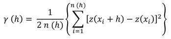
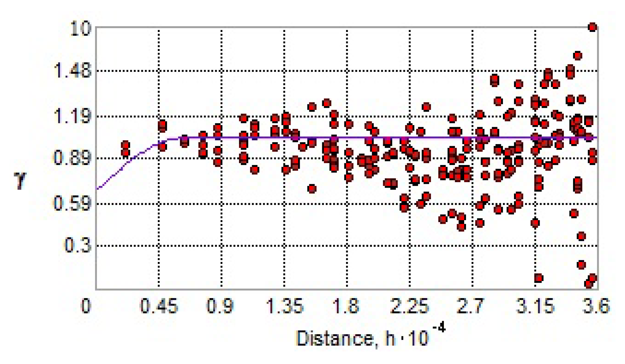
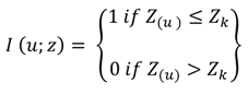
Geostatistics is a spatial statistical technique that can be used to assess and represent the distribution of concentration over space and time [7]. This technique predicts the estimated values based on the relationship between the sample points and estimates the uncertainty of that prediction [8,9,10]. Kriging is a linear interpolation procedure that is used to create probabilistic models of uncertainty relating to the values of the attributes. Indicator kriging (IK) is an efficient non-parametric geostatistical method with no assumption regarding the distribution of variables [11], and has the ability to take the data uncertainty into account and predict the conditional probability of certain data for an unsampled location [12]. Indicator kriging is also used to identify areas of high probability as potential sites for monitoring based on the current monitoring wells. However, this method alone is not sufficient for the optimal design of monitoring wells, without considering the potential risk from anthropogenic activities and the vulnerable hydrogeological characteristics. The vulnerability of groundwater is characterized by the hydrogeological and geological attributes of the aquifer [13] to specific areas that are more prone to contamination. The DRASTIC model is the most commonly applied vulnerability model based on the physical environmental aquifer parameters to assess groundwater vulnerability [14,15,16,17,18]. The existence of potential contamination activities should be considered as a risk for groundwater pollution since the vulnerability only represents the intrinsic characteristic of the aquifer. As the population of an area grows, intensive agricultural activities, inappropriate placement of commercial and industrial regions and high intensity residential areas can potentially cause pollution of the groundwater. Therefore, land use is an additional parameter that can be integrated into the DRASTIC method to evaluate the potential risk in different areas [13,15].

Few researchers have applied the integration of geostatistical techniques and vulnerability assessment as a new approach for redesigning the groundwater monitoring networks [5,19,20,21]. The density of monitoring wells was considered together with vulnerability assessments by Dawoud [22]. Yeh et al. [21] applied a genetic algorithm and the factorial kriging method for nine variables—electrical conductivity (EC), total dissolved solids (TDS), Cl⁻, Na⁺, Ca²⁺, Mg²⁺, SO₄²⁻, Mn, and Fe—for optimal selection of monitoring wells in Pingting Plain, Taiwan. To reach a similar objective, Baalousha [5] developed a new methodology by combining vulnerability and ordinary kriging maps based on the nitrate concentration from groundwater in the Heretaunga Plain, New Zealand. Preziosi et al. [20] developed a GIS based procedure to select the most appropriate monitoring points by combining the actual contamination data, the attributes of water points, and the vulnerability conditions for a variable density network design.

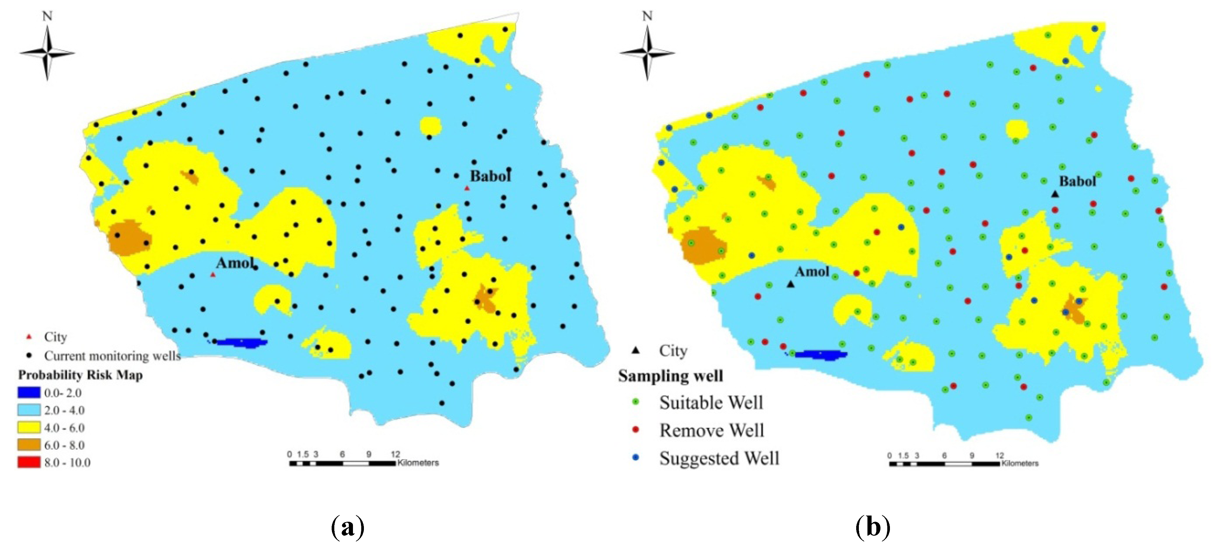
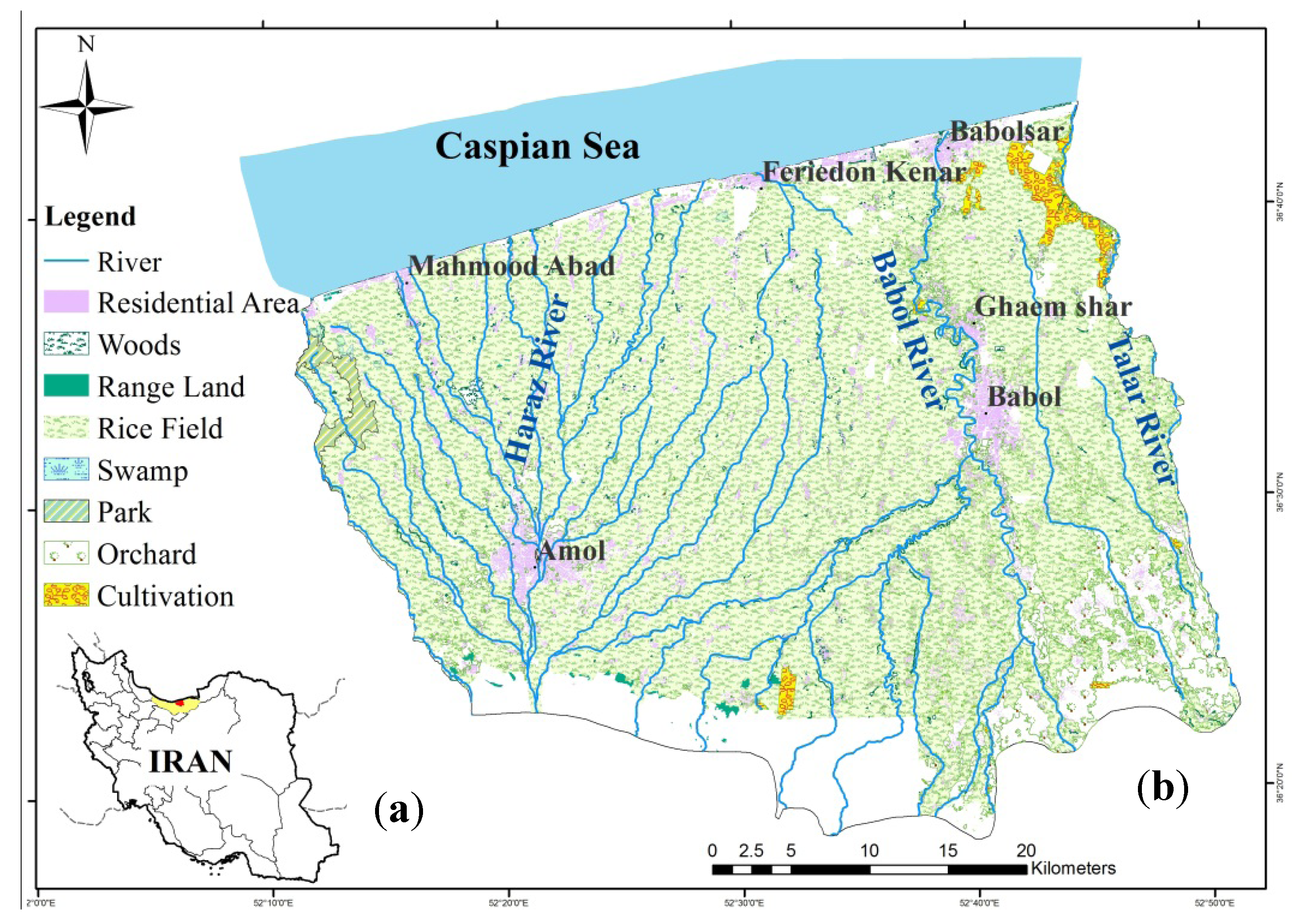
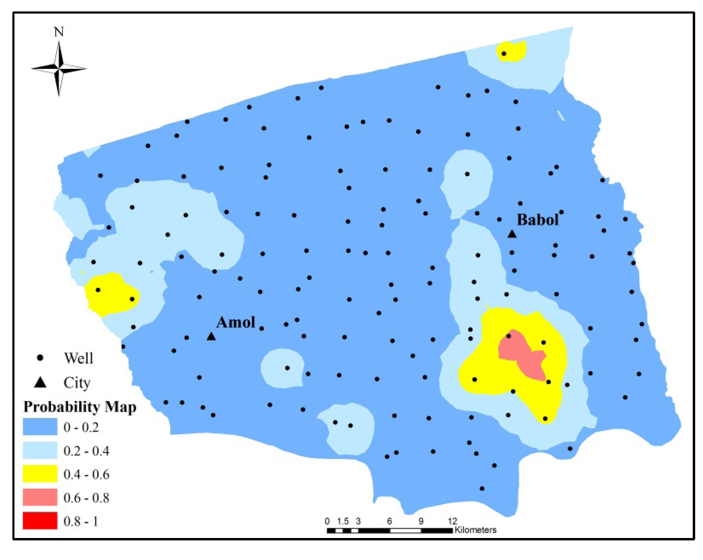
In this study, the data collected from 147 monitoring wells were applied to estimate the potential contamination risk of nitrate in drinking water using indicator kriging on the Amol-Babol Plain, in northern Iran. Moreover, the potential risk zones of groundwater to pollution are specified by integrating the vulnerability and risk mapping in the study area. The main purpose of this study was to develop a new approach to identify areas with high potential pollution and assess the efficiency of the current monitoring wells by probability risk assessment method.

2. Materials and Method

2.1. Study Area

The Amol-Babol Plain, which is situated in Mazandaran Province in the northern part of Iran, covers about 1822 km². The plain has a subtropical and humid climate with a hot summer. The annual mean temperature is 17.9 °C [23]. The average temperature decreases from the Caspian coastal area towards the Alborz Highlands in the southern region (Figure 1). The annual precipitation is about 880 mm with the majority of precipitation occurring during the rainy season (November and December).

Geomorphologically, the transportation and sediment deposition by the Haraz River, Talar River and Babol River (1b) have evolved into alluvial fans, marine deposits and a flood plain.

The agricultural land, which consists of irrigated fields, dry farming and orchards, covers around 51%, 12.8% and 8% of the Amol-Babol Plain, respectively (Figure 1) [23]. Groundwater constitutes 63% of the total water supply in the study area. The annual water abstraction is about 44 million m³ for domestic consumption and 390 million m³ for agricultural usage [23]. Water in the study area is abstracted from 61,496 shallow wells and 6634 deep wells. Huge amounts of fertilizer, mainly nitrates and phosphates, are applied by farmers to the agricultural land, especially in the first quarter of the year for the agricultural activities (Table 1).

Livestock is the second most important economic activity in the rural parts of the study area. Nitrogenous compounds are the main polluting components present in livestock waste [24]. Around 56,885 kg/day of nitrogenous compounds are produced by livestock in the area [23].

Figure 1. (a) Map of Iran; (b) Land use map of Amol-Babol Plain.

Figure 1. (a) Map of Iran; (b) Land use map of Amol-Babol Plain.

Table 1. Average of annual nitrate fertilizer usage in the study area [25].

Fertilizer	Paddy (Kg/ha)	Dry land farming (Kg/ha)	Citrus (Kg/ha)
Nitrate	207	122	200
Phosphate	180	139	405
Potash	77	187	304

Table 1. Average of annual nitrate fertilizer usage in the study area [25].

Fertilizer	Paddy (Kg/ha)	Dry land farming (Kg/ha)	Citrus (Kg/ha)
Nitrate	207	122	200
Phosphate	180	139	405
Potash	77	187	304

Runoff, containing nitrate, phosphate and coliforms from the livestock yards or irrigated land may infiltrate the groundwater, especially in areas with a shallow water table (less than 30 m [26], such as the Amol-Babol Plain.

2.2. Groundwater Sampling and Analysis

Groundwater nitrate content is highly related to soil type and geological conditions. Generally, the natural value of nitrate in groundwater should only be a few milligrams per liter [27]. Inorganic nitrogen in fertilizers, such as nitrate (NO₃⁻), ammonium (NH₄) and organic nitrogen in waste, break down to ammonia in the soil and then oxidize into nitrate. Nitrate is essential for plant growth and is used in the synthesis of organic nitrogen compounds [27,28]. When not all the nitrate is used by the plants, it may accumulate in the soil and infiltrate into the aquifer. Under anaerobic conditions in the aquifer, nitrate could be completely denitrified or degraded into nitrogen. In order to analyze the nitrate concentration in the groundwater of the Amol-Babol Plain, 147 water samples were collected from the groundwater monitoring wells in 2009. The initial selection of spatial distribution monitoring wells locations was mostly obtained from local experts based on their simple professional experience or empiric-type criteria of the possible sources of nitrate contamination in the study area. The groundwater was pumped out for 10 to 15 min to flush away the non-representative samples of polluted water. The groundwater samples were stored in polyethylene bottles [29] and kept at less than 4 °C in a refrigerator and were analyzed within 24 hours. Nitrate concentration was performed on groundwater samples according to APHA [29] using the colorimetric method.

2.3. DRASTIC Method

2.3.1. Vulnerability Assessment

The US Environmental Protection Agency (EPA) developed the DRASTIC model to standardize the methods for evaluating the vulnerability of groundwater to contamination [30]. Intrinsic groundwater vulnerability is an index and overlay method, which is dependent on the different hydrogeological parameters of the aquifer system [14]. Seven parameters—depth to water table, net recharge, aquifer media, soil media, topography, impact of vadose zone, and hydraulic conductivity (DRASTIC)—are applied by the model for assessing groundwater vulnerability.

A specific rate from 1 to 10 is assigned to each parameter, based on the hydrogeological characteristics (Table 2), with the higher values representing greater vulnerability potential. Then, weights are allocated to each of the seven hydrogeological settings from 1 to 5 (Table 2).

Table 2. DRASTIC parameters [30].

rating	(D)	(R)	(A)	(S)	(T)	(I)	(C)
	Depth to water (m)	Net recharge (mm)	Aquifer media	Soil media	Topography (% slope)	Impact of Vadose zone material	Conductivity (m/d)
1	>30.4	50.8	-	No shrinking Clay	>18	Confining layer	0.04–4.1
2	22.8–30.4	-	Massive shale	Muck	-	-	4.1–12.3
3	15.2–22.8	50.8–101.6	Metamorphic igneous clay	Clay loam	12–18	Silt/clay Shale limestone	-
4	-	-	Weathered metamorphic	Silty loam	-	-	12.3–28.7
5	9.1–15.2	-	Glacial till	Loam	6–12	-	-
6	-	101.6–177.8	Bedded sandstone limestone	Sandy loam	-	Sandstone bedded limestone and limestone shale, gravel and w. silt	28.7–41
7	4.6–9.1	-	-	Shrinking clay	-	-	-
8	-	177.8–254	Massive limestone sand and gravel	Peat	-	Sand and gravel	41–82
9	1.5–4.6	-	basalt	Sand	2–6	Basalt	-
10	0–1.5	>254	Karsts limestone	Thin or absent Gravel	0–2	Karsts limestone	>82
weight	5	4	3	3	1	5	3

Table 2. DRASTIC parameters [30].

rating	(D)	(R)	(A)	(S)	(T)	(I)	(C)
	Depth to water (m)	Net recharge (mm)	Aquifer media	Soil media	Topography (% slope)	Impact of Vadose zone material	Conductivity (m/d)
1	>30.4	50.8	-	No shrinking Clay	>18	Confining layer	0.04–4.1
2	22.8–30.4	-	Massive shale	Muck	-	-	4.1–12.3
3	15.2–22.8	50.8–101.6	Metamorphic igneous clay	Clay loam	12–18	Silt/clay Shale limestone	-
4	-	-	Weathered metamorphic	Silty loam	-	-	12.3–28.7
5	9.1–15.2	-	Glacial till	Loam	6–12	-	-
6	-	101.6–177.8	Bedded sandstone limestone	Sandy loam	-	Sandstone bedded limestone and limestone shale, gravel and w. silt	28.7–41
7	4.6–9.1	-	-	Shrinking clay	-	-	-
8	-	177.8–254	Massive limestone sand and gravel	Peat	-	Sand and gravel	41–82
9	1.5–4.6	-	basalt	Sand	2–6	Basalt	-
10	0–1.5	>254	Karsts limestone	Thin or absent Gravel	0–2	Karsts limestone	>82
weight	5	4	3	3	1	5	3

The most important parameters have a weight of 5 and the least important have a weight of 1. The DRASTIC index is calculated by multiplying each factor’s rating by the assigned weights, as follows:

DRASTIC Index = D_RD_W + R_rR_w + A_rA_w + S_rS_w + T_rT_w + I_rI_w + C_rC_w

(1)

where D, R, A, S, T, I, and C represent the seven hydrogeological factors, r is the rating and w the weight. The DRASTIC index represents a relative measure of groundwater vulnerability and can range from 26 (very low vulnerability) to 226 (extremely high vulnerability) [31].

Although areas with a low DRASTIC index are less susceptible to pollution compared to areas with a high DRASTIC index, it does not mean that these areas are completely free from groundwater contamination. The DRASTIC model is based on four assumptions: (a) the contaminant is introduced at the ground surface; (b) the contaminant enters the groundwater by precipitation; (c) the contaminant has mobility; and (d) the area should be 400 m² or larger [15].

2.3.2. Risk Assessment

The risk of groundwater contamination is not only determined by the intrinsic groundwater vulnerability map, but is also related to the existence of contamination sources. Human activities, which mainly occur at the land surface, could be the source of groundwater contamination. To assess the potential risk of groundwater, an extra factor (land use) should be added to the study (Table 3). The risk map was created based on the following equation [17]:

Risk Index = DRASTIC index + L_rL_w

(2)

where L refers to land use, r to the rating and w to weight. Secunda et al. [32] and Adamat et al. [17] specified three dominant classes of land use activity—built-up area, irrigated field crops and uncultivated land—that could affect groundwater quality (Table 3).

Similar to the vulnerability map, the groundwater contamination risk map could be classified into eight classes, from very low (<145) to extremely high (>270) contamination risk (Table 4) [33].

Table 3. Land use classification [17].

Land use activity	Rating
Irrigated field crop	8
Built-up area	8
Uncultivated land	5
Land use weight	5

Table 3. Land use classification [17].

Land use activity	Rating
Irrigated field crop	8
Built-up area	8
Uncultivated land	5
Land use weight	5

Table 4. Classification of vulnerability and risk index values.

class	Very low	low	Moderate low	Moderate	Moderate high	High	Very high	Extremely high
Total Drastic index value	27–79	80–99	100–119	120–139	140–159	160–179	180–199	199–240
Total risk index value	<145	145–165	166–186	187–207	208–228	229–249	250–270	>270

Table 4. Classification of vulnerability and risk index values.

class	Very low	low	Moderate low	Moderate	Moderate high	High	Very high	Extremely high
Total Drastic index value	27–79	80–99	100–119	120–139	140–159	160–179	180–199	199–240
Total risk index value	<145	145–165	166–186	187–207	208–228	229–249	250–270	>270

2.4. Geostatistical Technique

2.4.1. Variogram Analysis

Geostatistics have been defined by Matheron [34] as “the application of probabilistic methods to regionalized variables,” indicating that any variable in an area has both random and spatial properties [35]. This technique was developed to create mathematical models for a spatial correlation structure [34,35,36] with a variogram that quantifies the spatial variability of random variables between two points [37]. The empirical semivariogram, γ_(h), is calculated as half the average quadratic difference between data points separated by the distance vector h [35]:

(3)

where n (h) is the total number of the variable pairs separated by this distance; and z (x) is the value of the variable.

The experimental variogram is fitted into a theoretical model, which comprises eleven different functions: circular, spherical, tetra spherical, pentaspherical, exponential, Gaussian, rational quadratic, Hole effect, K-Bessel, J-Bessel and stable. The cross validation estimation is applied as the goodness-of-fit method for selecting the best variogram model. For accurate prediction, the mean error (ME) and kriged reduced mean squared error (KRMSE) are computed as follows:

(4)

(5)

where Z_0,i is the observed value at location I; Z_p,i is the predicted value at the location i; and N is the number of observations and predicted value; S is the standard deviation of the observed value. The corresponding sill (C₀ + C), nugget (C₀), and range values of the best-fitting theoretical model are observed. The nugget–sill ratio is utilized in the classification of the spatial dependency of groundwater quality parameters [38].

The variogram can be computed in different directions to detect any anisotropy of the spatial variability. An anisotropic model generally includes geometric anisotropy and zonal anisotropy [39].

2.4.2. Indicator Kriging

Indicator kriging (IK) is applied as a non-parametric geostatistical method to approximate the conditional cumulative distribution function at an unsampled point based on the correlation structure of indicator-transformed data points [11]. The indicator kriging function of the observation Z(u) at point u related to the threshold value Z is formulated as follows [11,40]:

(6)

where Z_k is the threshold level.

The expected value of I (u;z_k), conditional on n surrounding data, is written as:

E [I (u; z_(k)|(n))] = prob {z_(u) ≤ z_(k)|(n)) = F (u; Z_(k)|(n))}

(7)

where F (u; Z_(k)|(n)) is the conditional cumulative distribution function of Z_(u) ≤ Z_(k). Indicator kriging is a form of estimation methodology, in which the method is based on an estimator represented as:

(8)

where I (U_j ; Z_k) expresses the mount of the indicator at the measured point, U_j, j = 1, 2… n, and λ_j is a weighting factor of I (U_j ; Z_k) used in estimating I (U₀ ; Z_k).

The geostatistical extension module of ArcGIS 9.3 was used for the indicator kriging estimation in this study [10].

3. Results and Discussion

3.1. Groundwater Vulnerability and Risk Map

In order to assess a vulnerability map, the parameters of the DRASTIC model were prepared using ArcGIS software [10].

‒ Depth to water (D)

The depth to water is one of the significant parameters for determining the distance between the land surface and the groundwater level, through which the contaminants percolate to the groundwater. This layer was obtained using the kriging method for the water depth values measured in 2008. The groundwater depth on the Amol-Babol Plain varies between 2 m and 59.8 m. The shallow wells are mostly located near the coastal area at the northern side and the deep wells are found along the western and southern parts of the study area. Shallow wells have a rating of about 9 (D varies between 1.5 and 4.6) because the groundwater could easily be contaminated by surface runoff and contaminants (Table 2).

‒ Net Recharge (R)

The net recharge is the amount of water available from precipitation and artificial sources that can penetrate to the groundwater levels [41]. The net recharge layer was obtained by calculating the minimum, maximum, and mean value of net recharge using the Guttman Equation [42], as follows:

(9)

where, R is annual recharge and P is precipitation, both in millimeters.

The average annual rainfall is around 800 mm in 2010. Therefore the net recharge was estimated to be about 350 mm, which is classified in rate 10 (Table 2), for each weather station in the Amol-Babol Plain. The final layer was obtained using the kriging method and the raster map was classified using the rating in the ArcGIS environment.

‒ Aquifer media (A)

Aquifer media refers to the lithology of the saturated zone [43], which was obtained in the study area from the database of the boreholes and wells. The groundwater flow system is influenced by aquifer media, due to the role of rocks or sediment in a formation or group of formations to transfer quantities of water to wells and springs [30]. Sandstone, gravel, and silt are the main lithological components of the aquifers from the Amol-Babol Plain. In this layer, the highest rating is 8, which represents the sand and gravel layer (Table 2) along the western side of the study area. The rating is about 6 for the bedded sandstone (Table 2), which is found in the central and along the southern side of the area. The lowest rating is 3, which indicates a clay layer in the limited area of the north and northeastern side of the Amol-Babol Plain. A raster map of the aquifer was obtained by interpolating between the rate values and reclassified into three groups, including the gravel layer, bedded sandstone and clay layer.

‒ Soil media (S)

Soil media forms the uppermost part of the vadose zone, and influences the potential contamination [44]. Soil data were driven from the area soil reports [23]. The predominant soil in the Amol-Babol Plain was found to be river alluvium. The soil varies gradually from coarse-grained soils, mainly gravel and sand in the highlands, to fine-grained soils, mainly silts and clays, in the coastal area on the northern side of the study area. Therefore, classes 4, 5 and 6 were the identified rates according to silty loam, loam, and sandy loam, respectively, and 9 for sandy soil (Table 2).

‒ Topography (T)

The topography represents the slope of the land surface. This layer was created using digital elevation model (DEM) maps of the Amol-Babol Plain. In low slope areas there is increased infiltration from runoff, which shows greater potential for groundwater contamination, while high slope areas, cannot retain runoff for a long time reducing infiltration to the groundwater. The topography rating changed from 10 for most parts of the plain to 1 for the highlands on the southern side of the study area.

‒ Impact of the vadose zone

The vadose zone is the ground portion found between the aquifer and the soil cover in which pores or joints are unsaturated, depending on its permeability and the attenuation characteristics of the media [41]. The duration of the movement of contaminants into the groundwater is influenced by the zone’s components. Lithological and geophysical data from boreholes [23] indicates the presence of silt, clay, shale, and gravel in the vadose zone of the study area. A lower rating (rating 3) is assigned for clay and silt, as they present a less penetrable layer. Larger grain sizes, such as gravels and shales, show higher permeability and lower ability to filter contamination [41]. Therefore, a rating of 8 is assigned to the shale and gravel layer (Table 2), which covers the southern part of the Amol-Babol Plain.

‒ Hydraulic conductivity (C)

This parameter represents the ability of the aquifer to transmit water and also controls the rate of contaminant migration from the source to the aquifer [30]. Hydraulic conductivity values were calculated based on the transmissibility data from pumping wells and also the thickness of the aquifer from geophysical data. This parameter was computed based on the following equation:

(10)

where k is the hydraulic conductivity (m/d), T is the transmissivity (m²/d), and b represents the thickness of the aquifer (m).

The transmissivity values vary from 100 m²/d on the northern and northeastern parts to more than 2000 m²/d in the southern and southwestern parts of the Amol-Babol Plain. The aquifer thickness also changes from 25 m in the north to more than 300 m in the west and southwestern side. Therefore, the hydraulic conductivity in the plain varies from 0.04 m/d to 16.4 m/d. The interpolation method was used to create a raster map, which was classified into rates 1, 2 and 4 (Table 2) to create the conductivity map of the study area.

‒ Vulnerability mapping

The integration of the seven obtained maps, after multiplying each map with the respective related rating and weights (Equation (1)), provides the vulnerability to contamination map for the Amol-Babol Plain (Figure 2a). The minimum and maximum DRASTIC index could be varied between 27 and 240, respectively (Table 4). This range was divided into 8 equal classes, from very low to extremely high vulnerability. The resulting DRASTIC scores from the study area vary between 107 and 169, and were categorized as: 107–119 = moderate low vulnerability (representing 9.4% of the area), 120–139 = moderate vulnerability (representing 72% of the area), 140–159 = moderate high vulnerability (representing 17.06% of the area), and 160–169 = high vulnerability (representing 1.54% of the area). Most of the study area presents moderate and moderate low vulnerability (Figure 2a). The moderate high vulnerable areas occur in the western and northwestern parts, while the highest vulnerability area is located along the western side (Figure 2a).

Figure 2. Groundwater vulnerability map (a); and risk map (b) of the Amol-Babol Plain.

Figure 2. Groundwater vulnerability map (a); and risk map (b) of the Amol-Babol Plain.

‒ Risk mapping

Land use is an additional parameter that can be integrated into the vulnerability parameters for the potential risk of groundwater contamination. Amol-Babol Plain is mostly covered by irrigated field crops, orchards, marsh, and forests. Therefore, the elements presenting risk are mainly agricultural activities and urban development. The highest weight (5) was used for the land use layer, and a specific rate was assigned to each category (Table 3) based on the significance of the pollution potential contamination for each class. The land use layer for the Amol-Babol Plain shows that agricultural lands and urban areas are the dominant land uses covering 1760 km² of the 1822 km² total area, and, therefore, were assigned a rating of 8. The resulting risk scores vary between 141 and 211, and the areas are classified as a very low to moderately high risk index area (Table 5). Most of the area corresponds to low to moderate risk zones (Figure 2b).

Table 5. Distribution of risk zones in the Amol-Babol Plain.

Risk index	Risk range	Area (km2)	Percent of total area (%)
Very low	<145	4.7	0.25
Low	146–165	601.2	33
Moderate low	166–186	1005.7	55.2
Moderate	187–207	210	11.5
Moderate high	207–211	0.92	0.05

Table 5. Distribution of risk zones in the Amol-Babol Plain.

Risk index	Risk range	Area (km2)	Percent of total area (%)
Very low	<145	4.7	0.25
Low	146–165	601.2	33
Moderate low	166–186	1005.7	55.2
Moderate	187–207	210	11.5
Moderate high	207–211	0.92	0.05

3.2. Groundwater Probability Map

Indicator kriging was applied to create a probability map for nitrate concentration in the groundwater of the Amol-Babol Plain. The measured data at each sampling well were subjected to a continuous scale and converted to a discrete indicator variable with a value of either “1” or “0”. Arslan and Demir [2] noted that the difference between variogram results may be due to the weather conditions, irrigation or drainage system of the study area. The best-fitting theoretical models and related semivariogram parameters were chosen to obtain the most accurate estimation, by evaluating eleven different models. The cross-validation was undertaken to determine the difference between the measured and estimated nitrate values in the groundwater, and the spherical semivariogram model was the best-fitting model (Figure 3 and Table 6). The cross-validation, which represents the accuracy of the predictions, shows that the mean error of nitrate in the groundwater is close to 0 (0.002) and that the root mean square standardized is close to one (1.006).

Table 6. Cross-validation and semivariogram model parameters for probability map of nitrate concentration.

Groundwater Parameter	Best-Fitted Model	Nugget (C0)	Sill (C0 + C)	R2	Mean	KRMSE
Nitrate	Spherical	0.0664	0.1126	0.58	0.002	1.006

Table 6. Cross-validation and semivariogram model parameters for probability map of nitrate concentration.

Groundwater Parameter	Best-Fitted Model	Nugget (C0)	Sill (C0 + C)	R2	Mean	KRMSE
Nitrate	Spherical	0.0664	0.1126	0.58	0.002	1.006

Figure 3. Experimental variogram of nitrate concentration and the fitting of theoretical model.

Figure 3. Experimental variogram of nitrate concentration and the fitting of theoretical model.

Around 11.7% of the measured nitrate concentration is higher than 10 mg/L NO₃⁻ N. This level of nitrate–nitrogen is equivalent to 45 mg/L of nitrate. The drinking water standard based on health risk was set to 10 mg/L NO₃⁻ N [17,27]. This value was used as the threshold value for human consumption. Concentrations lower than the threshold value were assigned 0, while the higher threshold was assigned as 1.

The potential of nitrate leaching from the soil to the groundwater depends on the amount of rainwater, soil type and well depth. The probability range is classified between very weak (0.0–0.2) and very strong (0.8–1.0) (Table 7 and Figure 4).

Table 7. Probability ranges of area exceeding groundwater nitrate threshold by indicator kriging.

Probability range	Description	Area
		(km2)	(%)
0.0–0.2	Very weak	1244.3	43
0.2–0.4	Weak	461.5	25.32
0.4–0.6	Moderate	103.9	5.7
0.6–0.8	Strong	12.3	0.67
0.8–1.0	Very strong	-	-

Table 7. Probability ranges of area exceeding groundwater nitrate threshold by indicator kriging.

Probability range	Description	Area
		(km2)	(%)
0.0–0.2	Very weak	1244.3	43
0.2–0.4	Weak	461.5	25.32
0.4–0.6	Moderate	103.9	5.7
0.6–0.8	Strong	12.3	0.67
0.8–1.0	Very strong	-	-

Figure 4. Probability map of nitrate concentration in the Amol-Babol Plain.

Figure 4. Probability map of nitrate concentration in the Amol-Babol Plain.

The probability map of nitrate shows two vulnerable zones—the northwestern and southern sides of the plain (Figure 4)—which cover around 116.2 km² (6.37) of the total area. About 12.3 km² in the southern part of Babol City was classified as highly vulnerable, as the nitrate concentration in the area exceeded the threshold limit (0.6 to 0.8) (Figure 4 and Table 7). About 103.9 km² (5.7%) shows a “moderate” probability of exceeding the threshold value, occurring around the north and northwest area of Amol City, the southern part of Babol City, and the northeastern part of the plain (Figure 4). There is no specific pattern on the area covered by a strong probability (Figure 4), which could be due to the source of nitrate contamination. Domestic sewage and industrial wastewater coupled with an excessive use of fertilizers pose a nitrate hazard to the groundwater of the area.

The amount of infiltration also depends on the groundwater depth. Nitrate concentration is directly related to the extent of irrigation near the well and inversely to the well depth [45]. The shallow wells of less than 30 m deep constitute 60.3% of the sampling wells in the Amol-Babol Plain, which are the most vulnerable to nitrate contamination. However, about 1700 km² of the total area is suitable for drinking purposes, and the probability of exceeding nitrate concentration threshold is “weak” and “very weak” (Figure 4 and Table 7).

3.3. Monitoring Network Assessment

An approach to optimize the groundwater quality monitoring network was obtained using the hydrogeological setting and geostatistics. To achieve this purpose, we used a combination of risk mapping to identify vulnerable areas and probability maps to select areas with insufficient or maybe redundant information. The probability risk map was obtained using a combination of risk and probability maps, which were re-classified into 5 classes (from 1 to 5) to avoid any bias (Figure 5a). The risk map was re-classified from 1 (very low risk) to 5 (moderate high risk) according to Table 5. The probability map of nitrate concentration was also re-classified from 1 (very weak probability) to 5 (very strong probability) based on Table 4. In the probability risk map, the study area was classified from 2 to 7 (Table 8). The highest combined index represents areas with a very strong probability of nitrate concentration and moderate-high risk of contamination (Table 8). The areas with the highest classes should be monitored carefully and more stringently than the areas with lower indexes. However, this index was not observed in the combined map of the Amol-Babol Plain (Table 8). Otherwise, it was found that there is no monitoring well station in the combined index from 6.0 to 8.0 with moderate risk and strong probability areas in the southern part of Babol City and the northwestern side of Amol City.

Moreover, in the area with a combined index between 6.0 and 8.0, in the northwest of Amol City, the distance between two monitoring network wells was found to be more than 3.5 km. An area of 30 km² in the northeastern part of the plain with a moderate probability of nitrate concentration and moderate low risk has only one monitoring well. Furthermore, no monitoring well was considered for the northwestern part of the study area. Therefore, the monitoring network should be expanded in the aforementioned areas to provide accurate water quality monitoring and prevent a shortage of information. Additional monitoring wells could be chosen from those agricultural wells that have not been selected for previous monitoring networks (Figure 5b).

Figure 5. Combined probability map of nitrate concentrations and risk map of pollution (a); Suggested monitoring network (b).

Figure 5. Combined probability map of nitrate concentrations and risk map of pollution (a); Suggested monitoring network (b).

Table 8. Classification of probability risk map of nitrate contamination.

Probability risk index	Description	Area (km2)	Area (%)
0.0–2.0	Very low risk and very weak probability	4.76	0.26
2.0–4.0	Low risk and weak probability	1343.67	73.74
4.0–6.0	Moderate low risk and moderate probability	450.54	24.72
6.0–8.0	Moderate risk and strong probability	23.22	1.28
8.0–10.0	Moderate high risk and very strong probability	-	-

Table 8. Classification of probability risk map of nitrate contamination.

Probability risk index	Description	Area (km2)	Area (%)
0.0–2.0	Very low risk and very weak probability	4.76	0.26
2.0–4.0	Low risk and weak probability	1343.67	73.74
4.0–6.0	Moderate low risk and moderate probability	450.54	24.72
6.0–8.0	Moderate risk and strong probability	23.22	1.28
8.0–10.0	Moderate high risk and very strong probability	-	-

The extensive areas located in the northern, southern, and eastern parts of the plain have a low-class value with low risk and weak probability of nitrate contamination. Near Babol City and the central part of the plain, the distance between the monitoring wells is less short than 800 m. The number of monitoring wells can be reduced in these areas to minimize redundant information and reduce monitoring costs (Figure 5b).

A monitoring network could be suggested based on 128 sampling wells, for future nitrate assessment in groundwater of the area. This can be achieved by adding 12 new wells in the high risk areas and removing 30 wells from the low risk areas.

Based on the risk map, the results show that part of the southern portion of Babol City was characterized as low risk, while in the probability map, the area was found to have a high probability of nitrate contamination. Hence, when the two maps were compared, it was found that the area has moderate to high probability risk. These results have proven that relying on a risk map alone may be misleading. Therefore, it is advisable to combine both maps to achieve reliable results.

A probability risk map, comprising the risk and probability maps of nitrate concentration from collected samples, is required to evaluate the efficiency of the initial groundwater quality monitoring networks and for redesigning the quality monitoring wells.

4. Conclusions

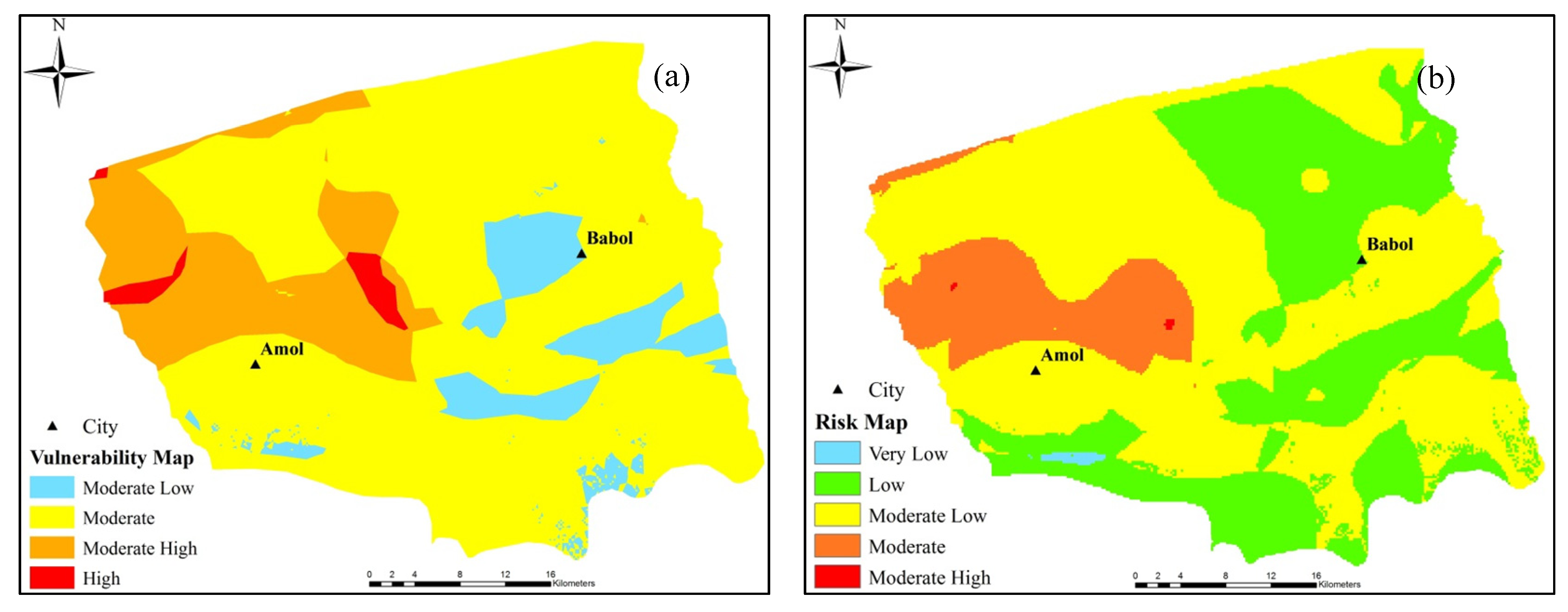
This paper developed an approach to assess and delineate areas that require groundwater quality monitoring. The proposed approach assesses the efficiency of the existing network of monitoring wells, considering not only the samples collected from the wells, but also the hydrogeological characteristics of the aquifer and the potential for anthropogenic pollution in the study area. The combination of indicator kriging to estimate the probability of nitrate concentration, together with the vulnerability and risk assessment by the DRASTIC method, represents a powerful and reliable method for identifying optimal sampling locations in the study area. The methodology was designed and successfully applied in the Amol-Babol Plain (Iran). The resultant map of the overlaid factors shows that some areas with strong nitrate probability and high risk of pollution on the south side of Babol City, the northeastern part of the plain and the northwestern part of Amol City are not covered by an adequate number of monitoring wells. However, the majority of the plain, which has a weak probability of nitrate concentration and low risk of contamination, is monitored by multiple sampling wells. Therefore, the existing monitoring wells should be reduced in the lower risk areas and increased in the areas with the highest risk of nitrate contamination. The proposed methodology is general and can be applied to any type of aquifer that is threatened by natural or anthropogenic pollution. In future studies, the proposed method could be applied to assess and redesign the monitoring wells based on various types of pollutants in the aquifer.

References

1. Jang, C.-S.; Chen, S.-K.; Kuo, Y.-M. Applying indicator-based geostatistical approaches to determine potential zones of groundwater recharge based on borehole data. Catena 2013, 101, 178–187. [Google Scholar] [CrossRef]
2. Arslan, H. Spatial and temporal mapping of groundwater salinity using ordinary kriging and indicator kriging: The case of Bafra Plain, Turkey. Agric. Water Manag. 2012, 113, 57–63. [Google Scholar]
3. Mogheir, Y.; Singh, V.P.; Lima, J.L.M.P. Spatial assessment and redesign of a groundwater quality monitoring network using entropy theory, Gaza Strip, Palestine. Hydrogeol. J. 2006, 14, 700–712. [Google Scholar]
4. Júnez-Ferreira, H.E.; Herrera, G.S. A geostatistical methodology for the optimal design of space-time hydraulic head monitoring networks and its application to the Valle de Querétaro aquifer. Environ. Monit. Assess. 2013, 185, 3527–3549. [Google Scholar] [CrossRef]
5. Baalousha, H. Assessment of a groundwater quality monitoring network using vulnerability mapping and geostatistics: A case study from Heretaunga Plains, New Zealand. Agric. Water Manag. 2010, 97, 240–246. [Google Scholar] [CrossRef]
6. Owlia, R.; Abrishamchi, A.; Tajrishy, M. Spatial-temporal assessment and redesign of groundwater quality monitoring network: A case study. Environ. Monit. Assess. 2011, 172, 263–273. [Google Scholar] [CrossRef]
7. Yeh, H.F.; Lee, C.H.; Hsu, K.C.; Chang, P.H. GIS for the assessment of the groundwater recharge potential zone. Environ. Geol. 2009, 58, 185–195. [Google Scholar]
8. Piccini, C.; Marchetti, A.; Farina, R.; Francaviglia, R. Application of indicator kriging to evaluate the probability of exceeding nitrate contamination thresholds. Int. J. Environ. Res. 2012, 6, 853–862. [Google Scholar]
9. Caridad-Cancela, R.; Vàzquez, E.V.; Vieira, S.R.; Abreu, C.A.; Gonzàlez, A.P. Assessing the spatial uncertainty of mapping trace elements in cultivated fields. Commun. Soil Sci. Plant Anal. 2005, 36, 253–274. [Google Scholar] [CrossRef]
10. Environmental Systems Research Institute (ESRI). Using ArcGIS Geostatistical Analyst; ESRI: Redlands, CA, USA, 2003. [Google Scholar]
11. Journel, A. Non-parametric estimation of spatial distribution. Math. Geol. 1983, 15, 445–468. [Google Scholar] [CrossRef]
12. Goovaerts, P. Comparative performance of indicator algorithms for modelling conditional probability distribution function. Math. Geol. 1994, 26, 389–411. [Google Scholar] [CrossRef]
13. Farjad, B.; Helmi, Z.M.S.; Thamer, A.M.; Pirasteh, S.; Wijesekara, N. Groundwater intrinsic vulnerability and risk mapping. Proc. ICE Water Manag. 2012, 165, 441–450. [Google Scholar] [CrossRef]
14. Babiker, I.S.; Mohamed, M.A.A.; Hiyama, T.; Kato, K. A GIS-based DRASTIC model for assessing aquifer vulnerability in Kakamigahara Heights, Gifu Prefecture, central Japan. Sci. Total Environ. 2005, 345, 127–140. [Google Scholar] [CrossRef]
15. Boughriba, M.; Barkaoui, A.; Zarhloule, Y.; Lahmer, Z.; Houadi, B.E.; Verdoya, M. Groundwater vulnerability and risk mapping of the Angad transboundary aquifer using DRASTIC index method in GIS environment. Arab. J. Geosci. 2010, 3, 207–220. [Google Scholar] [CrossRef]
16. Rezaei, F.; Safavi, H.; Ahmadi, A. Groundwater vulnerability assessment using fuzzy logic: A case study in the Zayandehrood Aquifers, Iran. Environ. Manag. 2013, 51, 267–277. [Google Scholar] [CrossRef]
17. Adamat, R.; Foster, I.; Baban, S. Groundwater vulnerability and risk mapping for the Basaltic aquifer of the Azraq basin of Jordan using GIS, remote sensing and DRASTIC. J. Appl. Geogr. 2003, 23, 303–324. [Google Scholar] [CrossRef]
18. Vias, J.; Andreo, B.; Ravbar, N.; Hotzl, H. Mapping the vulnerability of groundwater to the contamination of four carbonate aquifers in Europe. J. Environ. Manag. 2010, 91, 1500–1510. [Google Scholar] [CrossRef]
19. Chadalavada, S.; Datta, B. Dynamic optimal monitoring network design for transient transport of pollutants in groundwater aquifer. Water Resour. Manag. 2008, 22, 561–670. [Google Scholar]
20. Preziosi, E.; Petrangeli, A.B.; Giuliano, G. Tailoring groundwater quality monitoring to vulnerability: A GIS procedure for network design. Environ. Monit. Assess. 2013, 185, 3759–3781. [Google Scholar] [CrossRef]
21. Yeh, M.S.; Lin, Y.-P.; Chang, L.-C. Designing an optimal multivariate geostatistical groundwater quality monitoring network using factorial kriging and genetic algorithms. Environ. Geol. 2006, 50, 101–121. [Google Scholar] [CrossRef]
22. Dawoud, M.A. Design of national groundwater quality monitoring network in Egypt. Environ. Monit. Assess. 2004, 96, 99–118. [Google Scholar] [CrossRef]
23. Fakharian, K. Study of Prevention, Control and Reduce Pollution of Amol- Babol Aquifer; Hydrogeology Report of Amol-Babol Plain; Amirkabir University of Technology: Department of Environment of Iran: Tehran, Iran, 2010. [Google Scholar]
24. Goldberg, V.M. Groundwater pollution by nitrates from livestock wastes. Environ. Health Perspect 1989, 83, 19–25. [Google Scholar]
25. Ghods, M. Supplementary Environmental and Social Assessment of Alborz Intergrated Land and Water; Mahab Ghods Consulting Engineers: Tehran, Iran, 2004; p. 248. [Google Scholar]
26. McMahon, G.; Lloyd, O.B., Jr. Water-Quality Assessment of the Albemarle-Pamlico Drainage Basin, North Carolina and Virginia-Environmental Setting and Water-Quality Issues; U.S. Geological Survey Open-File Report; USGS: Denver, CO, USA, 1995; pp. 95–136. [Google Scholar]
27. World Health Organization (WHO). Nitrate and Nitrite in Drinking-Water, G.f.d.-w.q; Background Document for Development of WHO; WHO: Geneva, Switzerland, 2011. [Google Scholar]
28. Garner, B.D.; Mahler, B.J. Relation of Specific Conductance in Ground Water to Intersection of Flow Paths by Wells, and Associated Major Ion and Nitrate Geochemistry, Barton Springs Segment of the Edwards Aquifer, Austin, Texas, 1978–2003; USGS Scientific Investigations Report; USGS: Denver, CO, USA, 2007; p. 34. [Google Scholar]
29. APHA Standard Methods for the Examination of Water and Wastwater; American Public Health Association, American Water Workes Association, Water Environment Federation: Washigton, DC, USA, 2005.
30. Aller, L.; Bennet, T.; Lehr, J.H.; Petty, R. DRASTIC: A standardized System for Evaluating Groundwater Pollution Using Hydrogeologic Settings; 600/2-87-035; The US Environmental Protection Agency (EPA): Washigton, DC, USA, 1987. [Google Scholar]
31. Assaf, H.; Saadeh, M. Geostatistical assessment of groundwater nitrate contamination with reflection on DRASTIC vulnerability assessment: The case of the Upper Litani basin, Lebanon. Water Resour. Manag. 2009, 23, 775–796. [Google Scholar] [CrossRef]
32. Secunda, S.; Collin, M.; Melloul, A.J. Groundwater vulnerability assessment using a composite model combining DRASTIC with extensive land use in Israel’s Sharon region. J. Environ. Manag. 1998, 54, 39–57. [Google Scholar] [CrossRef]
33. Gomezdelcampo, E.; Dickerson, J.R. A modified DRASTIC model for siting confined animal feeding operations in williams county, Ohio, USA. Environ. Geol. 2008, 55, 1821–1832. [Google Scholar] [CrossRef]
34. Matheron, G. Les variables régionalisées et leur estimation; Masson: Paris, France, 1970. [Google Scholar]
35. Journel, A.; Huijbregts, C.J. Mining Geostatistics; Academic Press: New York, NY, USA, 1978. [Google Scholar]
36. Isaaks, E.H.; Srivastava, R.M. An Introduction to Applied Geostatistics; Oxford University Press: New York, NY, USA, 1989. [Google Scholar]
37. Antunes, I.M.H.R.; Albuquerque, M.T.D. Using indicator kriging for the evaluation of arsenic potential contamination in an abandoned mining area (Portugal). Sci. Total Environ. 2013, 442, 545–552. [Google Scholar] [CrossRef]
38. Uyan, M.; Cay, T. Geostatistical methods for mapping groundwater nitrate concentration. In Proceedings of the 3rd international conference on cartography and GIS, Nessebar, Bulgaria, 15–20 June 2010; 2010. [Google Scholar]
39. Deutsch, C.V.; Journel, A.G. GSLIB, Geostatistical Software Library and User’s Guide; Oxford University Press: New York, NY, USA, 1998. [Google Scholar]
40. Journel, A.; Keith, L.H. Non-Parametric Geostatistics for Risk and Additional Sampling Assessment, Principles of Environmental Sampling; American Chemical Society: Washington, DC, USA, 1988. [Google Scholar]
41. Rahman, A. A GIS based DRASTIC model for assessing groundwater vulnerability in shallow aquifer in Aligarh, India. Appl. Geogr. 2008, 28, 32–53. [Google Scholar] [CrossRef]
42. Guttman, J. Hydrogeology of the Eastern Aquifer in the Judea Hills and Jordan Valley; Multi-Lateral Project 02WT9719, Sub Project B, Final Report: Mekorot Report No. 468; Mekorot Co.: Tel-Aviv, Israel, 2000. [Google Scholar]
43. Saidi, S.; Bouri, S.; Dhia, H.B.; Anselme, B. A GIS-based susceptibility indexing method or irrigation and drinking water management planning: Application to Chebba—Mellouleche aquifer, Tunisia. Agric. Water Manag. 2009, 96, 1683–1690. [Google Scholar] [CrossRef]
44. Saidi, S.; Bouri, S.; Dhia, H.B. Groundwater vulnerability and risk mapping of the Hajeb-jelma aquifer (central Tunisia) using a GIS-based DRASTIC model. Environ. Earth Sci. 2010, 59, 1579–1588. [Google Scholar] [CrossRef]
45. Townsend, M.A.; Marks, E.T. Occurrence of nitrate in soil and ground water in south-central Kansas. In Proceedings of Ground Water Managementin Cluster of Conferences, Agricultural Impacts on Ground Water Quality Session, Kansas City, MO, USA, February 1990; pp. 145–158.