Long-Term Evolution of Cones of Depression in Shallow Aquifers in the North China Plain

Abstract

The North China Plain (NCP) is one of the places where the groundwater is most over-exploited in the world. Currently, our understanding on the spatiotemporal variability of the cones of depression in this region is fragmentary. This study intends to simulate the cones of depression in the shallow aquifer across the entire NCP during the whole period from 1960 to 2011. During the simulation, the dominant role of anthropogenic activities is emphasized and carefully taken into account using a Neural Network Algorithm. The results show that cones of depression in the NCP were formed in 1970s and continuously expanded. Their centers were getting deeper with an increasing degree of groundwater exploitation. This simulation provides valuable insights for developing more sustainable groundwater management options after the implementation of the South-to-North Water Diversion Project (SNWDP), which is a very important surface water project in China in the near future. The numerical model in this paper is built by MODFLOW, with pumpage data completed by neural network algorithm and hydrogeological parameters calibrated by simulated annealing algorithm. Based on our long-term numerical model for regional groundwater flow in the NCP, one exploitation limitation strategy after the implementation of SNWDP is studied in this paper. The results indicate that the SNWDP is beneficial for groundwater recovery in the NCP. A number of immense groundwater cones will gradually shrink. However, the recovery of the groundwater environment in the NCP will require a long time.

1. Introduction

Water shortage is a common phenomenon due to increasing population, expanding areas of irrigated agriculture and growing economic development. Groundwater is of fundamental significance to meet the increasing water demand [1]. However, the total global groundwater depletion has increased from 126 $k{m}^3{a}^{-1}$ in 1960 to 283 $k{m}^3{a}^{-1}$ in 2000 in subhumid to arid areas [2], owing to increased groundwater abstraction, especially in the world’s major agricultural regions, including northwest India, north China and the central USA [3]. When some of the negative effects begin to be noticed, certain management of aquifer would be implemented [3]. Therefore, understanding of processes of groundwater depletion under anthropogenic activities and climate change is significantly important for sustainable groundwater utilization [4]. Furthermore, the efficiency of implementing groundwater protection or recovery measures needs quantitative appraisal of aquifer evolution based on reliable data [3] and based on the relationship among different aquifers [5]. Numerical modeling of groundwater flow can provide quantitative insight into sustainability [6]. The North China Plain (NCP) is an excellent example covering these issues.

The NCP is one of the places in China that run short of groundwater resource. As China’s political, economic and cultural center, the NCP is a very important component in the country’s sustainable development strategy. Over the last fifty years, the number of pumping wells in the NCP has increased to more than 700,000 in 1997 [7], which is over 388 times larger than that in any year in the 1960s. Research indicates that anthropogenic activities are the dominant factor that controls the groundwater head changes including the distribution of cones of depression in the NCP [8,9]. The Quaternary aquifer of the NCP is traditionally divided into two aquifer zones referred as “shallow" and “deep" [10]. In the shallow aquifer of the NCP, between 1973 and 2003, the largest decrease in groundwater head is over 25 m [11], and the water table has a maximum overburden depth of 65 m [12].

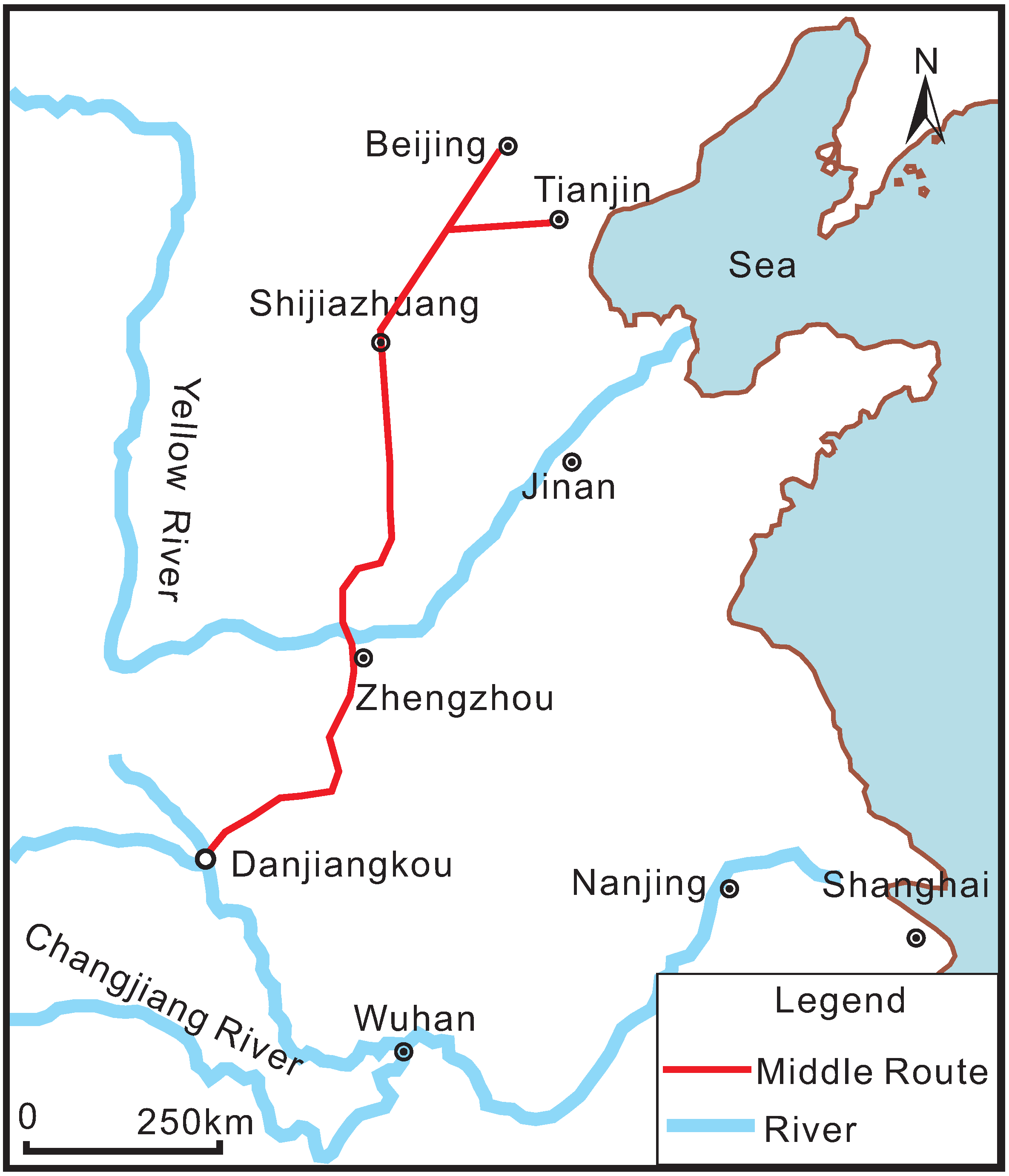
The middle route of the South-to-North Water Diversion Project (SNWDP) is supposed to be a significant method for the management and prevention of the continued shortage of groundwater resources in the NCP. It is a surface water project that conveys the water from Danjiangkou, which is in the branch of Yangzi River, to Beijing and Tianjin in the north via the main canal (Figure 1), the length of which is 1246 km [13]. The first phase of the middle route of the SNWDP will be completed after the flood season in 2014, supplying the North China with 13.4 billion $m^3$ of water [14]. The timetable of the second phase of the project has not been determined so far. The inflow of such large amounts of water into the NCP will significantly reduce groundwater mining, thus enabling sustainable groundwater management for the NCP.

Combined with other disciplines (such as agriculture [15], land use [16] and GIS [17]), numerical simulation of groundwater played an increasingly important role in the evaluation of groundwater sustainable yield and the prediction of groundwater flow field. Visocky studied the impact of Lake Michigan Allocations on the Cambrian-Ordovician aquifer system in the Chicago area by numerical simulation and concluded that water levels would partially recover in some areas while the major cones of depression would shift southward and westward and continue to spread outward [18]. Rubio et al. used two equilibrium concepts to analyze the maximum sustainable extraction amount of groundwater, groundwater cones would not expand under this estimated amount [19]. The numerical simulation of groundwater is not limited to middle or small scale areas. In recent years, research on groundwater simulation in complex large scale areas has become more and more popular [20].

Figure 1. Location of the middle route of the SNWDP.

Figure 1. Location of the middle route of the SNWDP.

In the NCP, several numerical models have been built to evaluate groundwater resources and flow dynamics.However, some of them are restricted to local areas or a certain period of the NCP. Jia and Liu used numerical modeling to evaluate groundwater level recovery in Luancheng in the piedmont region and estimated that reducing groundwater pumpage by 50 and 100 mm in the simulation period (January 1990 to December 1990) would result in water level recoveries of 0.25 and 0.56 m, respectively [7]. Feng et al. presented a decision support system, which is supported through simulation with an embedded water computable general equilibrium model, for assessing the social-economic impact of China’s SNWDP. They found that through an increment of water supply by the S2N Project and proper policy-making, the gap between water demand and supply can eventually be closed, and the cones of depression can therefore be recovered [21]. Liu et al. used a model to simulate flow dynamics from 1960 to 2004 to evaluate the effects of urbanization of rural areas in the vicinity of Shijiazhuang City and concluded that the SNWDP can only mitigate groundwater depletion in local areas [22]. Hu et al. integrated a crop-growth model and a groundwater model to evaluate the effects of reduction in irrigation in Shijiazhuang and estimated that 140 mm reduction in irrigation could stop groundwater depletion in this area [23]. Yang et al. built a numerical model to study the response of the groundwater system under Beijing to the SNWDP [24]. Zhang et al. assessed the evolution of groundwater circulation system and studied the past global changes in the NCP using analysis of groundwater dynamic field, simulation of groundwater geochemistry, $C^{14}$ dating and extraction of isotope information. They concluded that the water environment in the NCP has entered a new evolution stage in which it is intensely disturbed by the anthropogenic activities [25]. Wang et al. evaluated groundwater depletion in the NCP from January 2002 to December 2003 and estimated total inflow of 49.4 $k{m}^3$ relative to total outflow of 56.5 $k{m}^3$, resulting in a budget deficit of 7.1 $k{m}^3$ [26]. Cui et al. used groundwater modeling to evaluate effects of groundwater pumpage reductions in response to the SNWDP in 10 years of prediction period and estimated average groundwater level recovery rates of 2.1 m/year in the shallow aquifers in Shijiazhuang in the piedmont region and 0.8–1.5 m/yr in the deep aquifers in Dezhou in the central plain [27]. International researchers usually studied the NCP in cooperation with Chinese researchers. Foster et al. gave hydrogeologic and socio-economic diagnosis of groundwater resource issues in the NCP and identified strategies to improve groundwater resource sustainability [28]. Aji et al. analyzed the chemical and stable isotopes of the groundwater and surface water along the Chaobai River and Yongding River basin to identify the groundwater flow system in the NCP and found that groundwater in the NCP was controlled by the altitude effect, shallow groundwater belongs to the local flow system and deep groundwater part of the regional flow system [29].

The objective of this study was to use groundwater modeling to simulate spatiotemporal variability of the cones of depression in the shallow aquifers in the last half century and to evaluate potential exploitation limitation strategies after the implementation of the SNWDP in the future. In this study, groundwater dynamics in shallow aquifers were simulated across the NCP covering the whole post-development period (1960–2011) with the aid of two mathematical techniques, including the back-propagation Neural Network Algorithm to complete the missing data in pumpage and the simulated annealing method to obtain the optimized values for hydrogeological parameters while calibrating the model.

2. Methods

2.1. Method of Completing Missing Values in Pumpage

During the data collecting procedure, we found that the pumpage for some years between 1960 and 2011 were missing. Using detailed statistics about the population, the agricultural output value and the industrial output value in the NCP, we implemented the Back Propagation Neural Network Algorithm to restore the missing data of pumpage.

The Back Propagation Neural Network Algorithm was first proposed by Rumelhart and McCelland in 1986 [30]. It can learn and store the complex relationship between the inputs and outputs without knowing the explicit equation between them. This best fits our case, because there is no explicit equation between the inputs (the population, the agricultural output value and the industrial output value) and the output (pumpage) in our study, but we still want to retrieve the missing data in some years according to the data we have in other years.

The Back Propagation Neural Network consists of the input, the hidden layer and the output layer. The formula mapping the input to the hidden layer is as follows:

$$O_j=f(\sum W_{ij}\times X_i-q_j)$$

(1)

The formula mapping the hidden layer to the output layer is as follows:

$$Y_k=f(\sum T_{jk}\times O_j-q_k)$$

(2)

where f is a nonlinear function and $q_i$ is the threshold for the i th neural node. A choice for f is the continuous Sigmoid function between (0,1).

When new inputs enter the neural network, it can estimate the error between the expected values and the calculated values via the following formula:

$$E_p=1/2\times \sum {(t_k-Y_k)}^2$$

(3)

where $t_k$ is the expected value of the kth node and $Y_k$ is the calculated value of the kth node. Then, this error can be back-propagated to modify the weighting factors in the neural network by the following equation:

$$W_{ij}(n+1)=h\times {\varphi }_i\times Y_j+a\times W_{ij}\left(n\right)$$

(4)

where h is the learning coefficient, ${\varphi }_i$ is the error of the ith node, $Y_j$ is the calculated output of the jth node and a is the momentum factor. Hence, the neural network can be trained and eventually learn the complex relationship between the inputs and outputs.

2.2. Inversion for Hydrogeological Parameters

During calibration, hydrogeological parameters need to be adjusted to make the calculated groundwater levels fit the observed ones. Instead of adjusting the hydrogeological parameters manually, the simulated annealing method was used to obtain a global optimization solution [31].

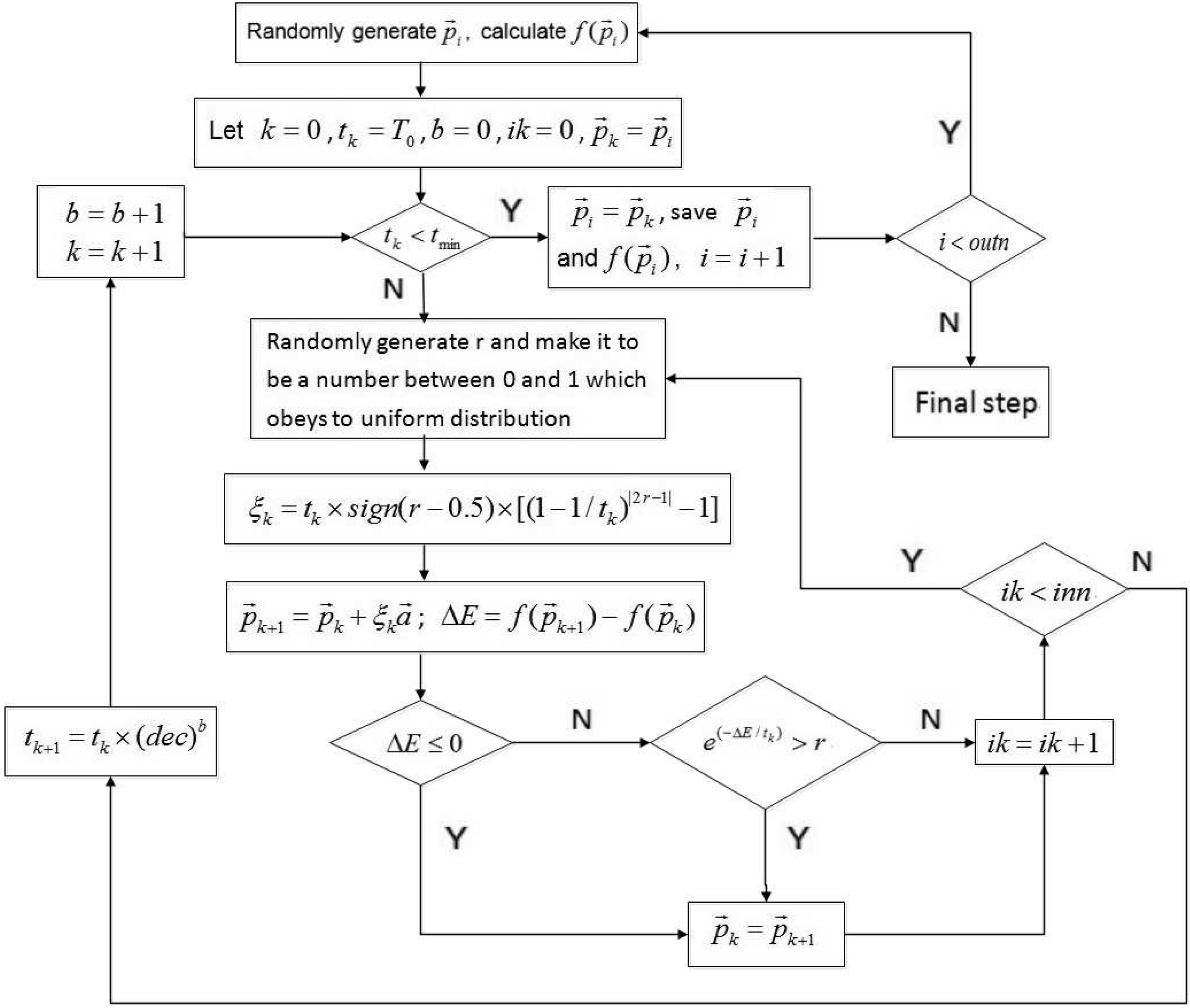
In the simulated annealing algorithm, firstly, we should build up a objective function $f\left(\overrightarrow{p}\right)$ according to the error estimation between the calculated and observed groundwater levels, where $\overrightarrow{p}$ is the vector formed by the hydrogeological parameters that are to be inverted. Set the parameters for the cooling down table. Give any initial temperature $T_0$ and initial solution ${\overrightarrow{p}}_0$, set $outn$ as the iteration number of outer loop, $inn$ as the length of Markov chain in inner loop and $dec$ as the decaying coefficient of temperature, give the range $\overrightarrow{a}$ of the variable hydrogeological parameters and the lowest temperature (cut-off temperature) $t_{min}$, set $i=0$. Then, we follow the work flow shown in Figure 2.

In the final step in Figure 2, we sort all the saved values of objective function corresponding to $outn$ approximations of optimal solution, and then choose the approximation that corresponds to the smallest value to be the global optimal solution $\overrightarrow{p}$ we want to find, which is the hydrogeological parameters we desire.

Figure 2. The loops in simulated annealing method.

Figure 2. The loops in simulated annealing method.

3. Numerical Model

3.1. Site Descriptions and Hydrogeological Setting

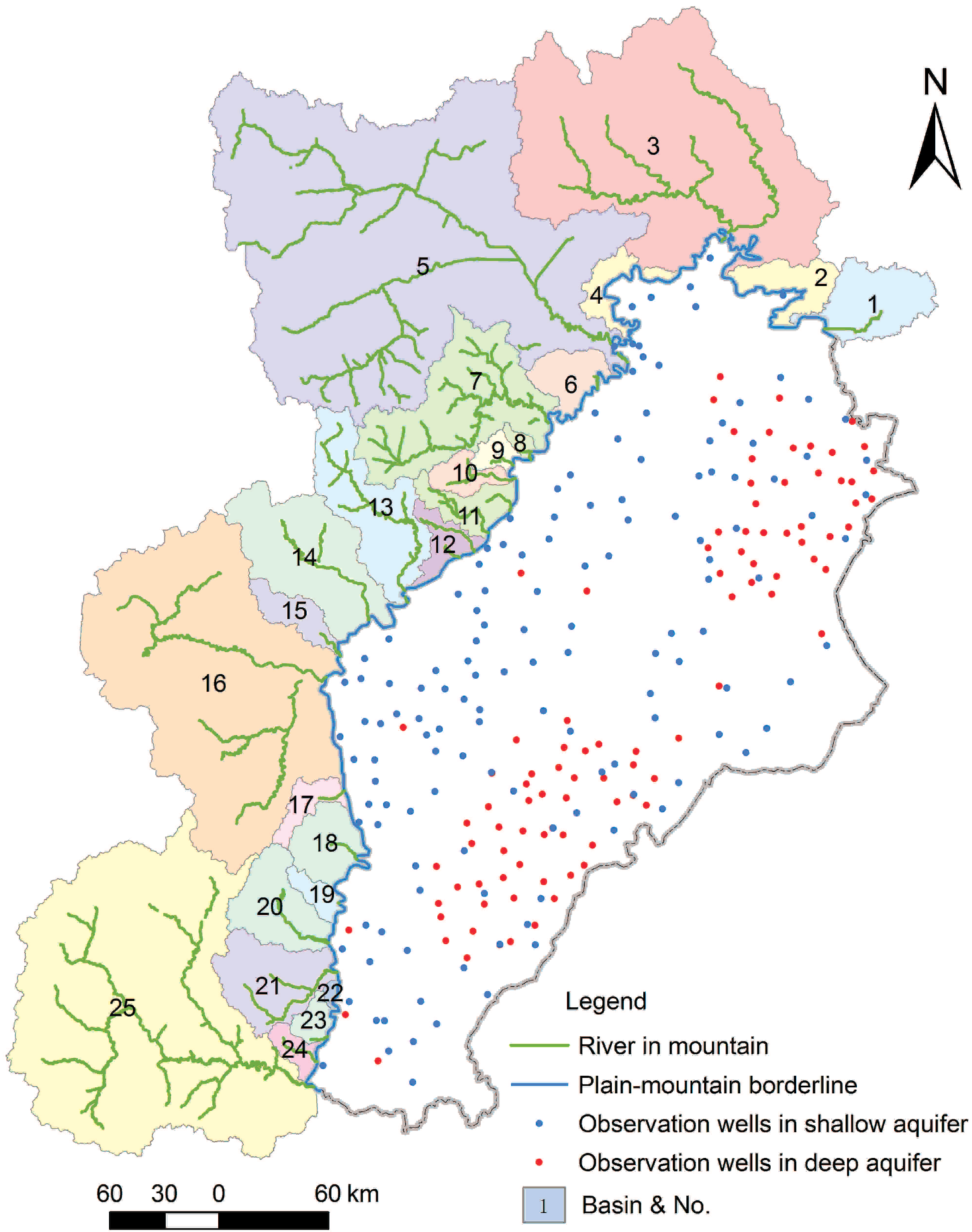
The study site includes two municipalities (Beijing and Tianjin) and one province (Hebei), with the Yan Mountain to the north, the Zhang River to the south, the Taihang Mountain to the west, and the Bohai Sea to the east, as shown in Figure 3a. The site encompasses an area estimated to be 80,592 $k{m}^2$ in total.

The study site lies in a warm temperate zone with semi-arid continental monsoon climate. The perennial mean precipitation is about 500–600 mm, with 75% of the rainfall concentrated in the flood season from June to September [26]. Mean annual pan evaporation ranges from 1000 to 2000 mm [11,26]. Because of the decrease in rainfall and the interception of upstream dams, most rivers have dried up since 1980s. Only a few rivers could flow for a short time in the flood season. Therefore, this region is seriously short of surface water [32].

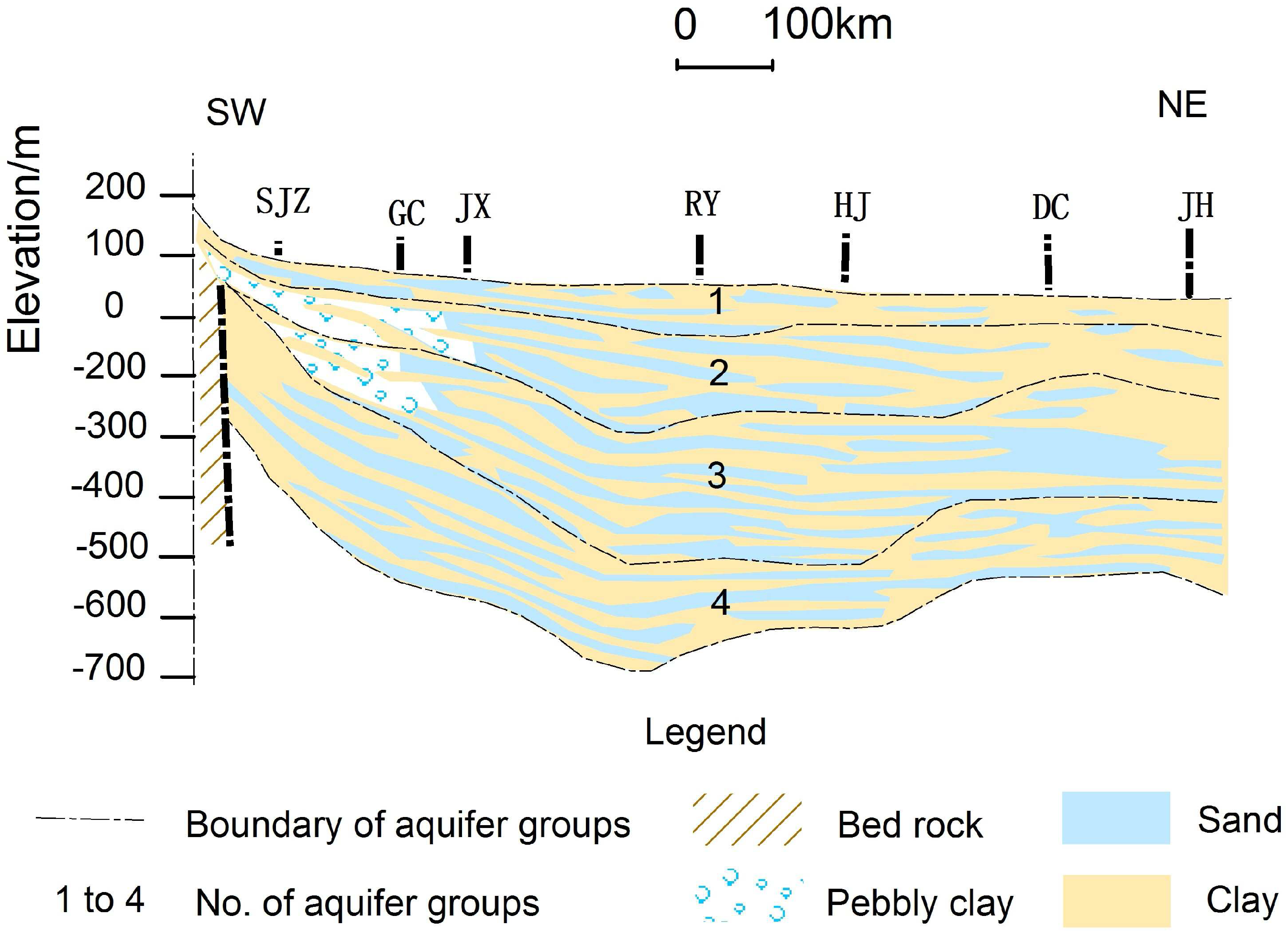
The Quaternary porous aquifer system in the NCP includes four aquifer groups [26,33] as shown in Figure 4. Aquifer groups 1 and 2 correspond to the shallow aquifer zone, and aquifer groups 3 and 4 correspond to the deep aquifer zone. The structure of the aquifers generally changes from a single layer to multiple layers, and the main lithologic characteristic of the aquifers changes from sand to clay from the piedmont plain to the littoral plain. Firstly, the main lithology of the piedmont plain is gravel and coarse sand. The aquifer is monolayer and yields a rich groundwater supply. Secondly, the main lithology of the central flood plain is fine sand and gravel, with overlapping aquifers. Finally, the main lithology of the coastal plain is silty sand and fine sand. Water is less abundant in this area compared with the two other hydrostratigraphic units [34].

Figure 3. Map of the study area: (a) shallow aquifer; (b) deep aquifer.

Figure 3. Map of the study area: (a) shallow aquifer; (b) deep aquifer.

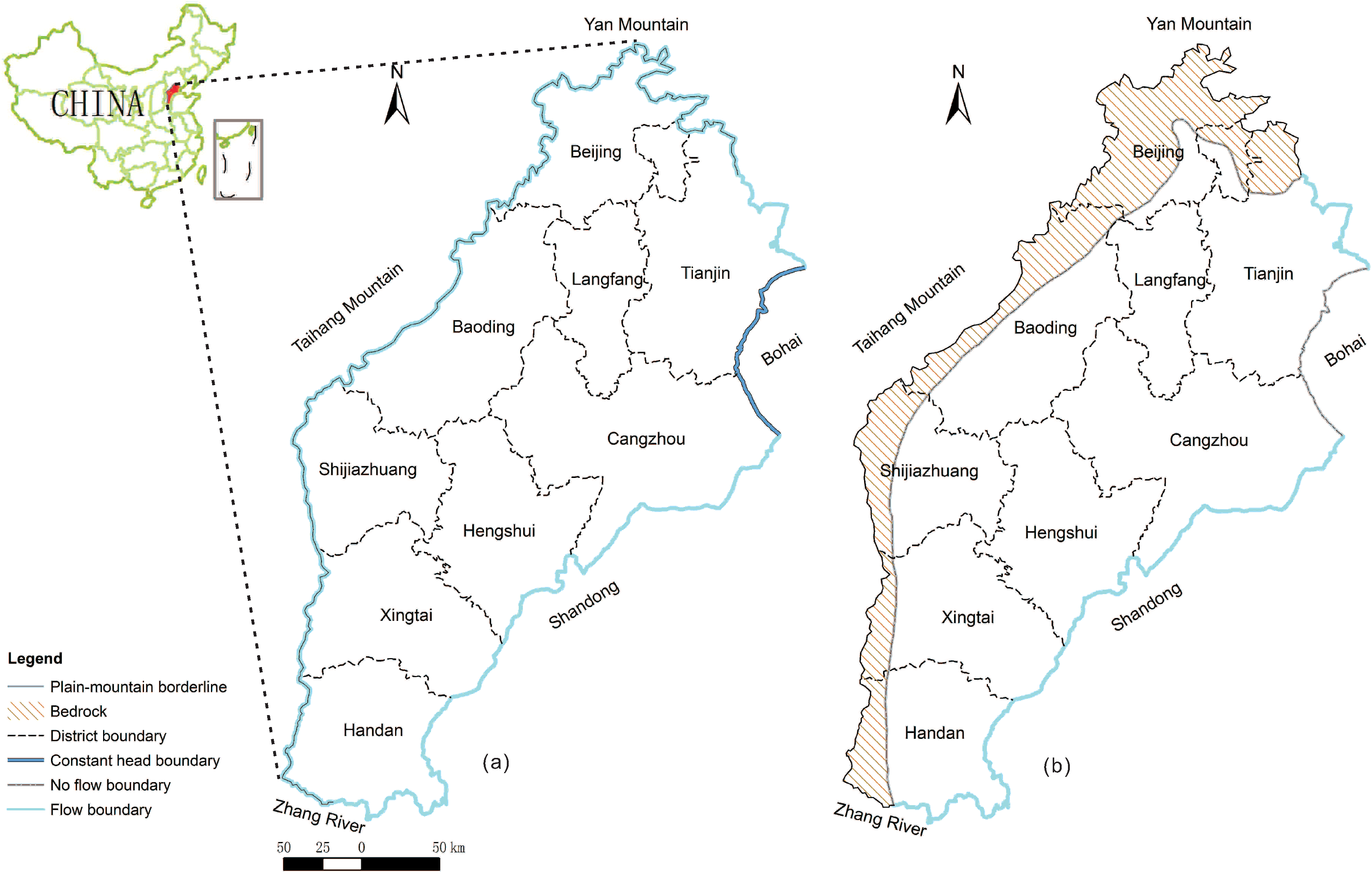
Figure 4. Schematic cross-section of the NCP [35].

Figure 4. Schematic cross-section of the NCP [35].

3.2. Model Discretization

A groundwater flow model in the NCP is established by using MODFLOW-2000 [36,37], the United States Geological Survey groundwater flow model. MODFLOW is a modular, three-dimensional finite-difference, groundwater flow code that simulates saturated porous media under steady-state and transient conditions [24]. The model has 188,706 active cells. One grid cell is 2 km × 2 km.

According to the hydrogeological condition and data on the porous aquifers at the study site, the model includes three anisotropic layers. In the model, layer 1 includes aquifer groups 1 and 2. Layer 2 includes aquifer group 3 and layer 3 includes aquifer group 4.

The simulation period is from 1960 to 2011. The temporal interval is 1 year. The observed field of groundwater in 1959 [38] is taken as the initial flow field in the model.

3.3. Boundary Conditions

As shown in Figure 3, the boundary along the coastline of the Bohai Sea is defined as constant head, and the other boundaries are flow boundaries in the first layer. Lateral boundaries for layers 2 and 3 are assumed to be no flow [11]. The vertical direction exhibits infiltration of precipitation, irrigation and surface water leakage, as well as phreatic water evaporation on the surface of the water table [11].

3.4. Recharge and Discharge

The lateral supply boundary, which is denoted as the light blue line in Figure 5, is between the mountains and the NCP [39]. The recharge R from mountains to the NCP through this boundary can be estimated by $R=Q-C-S$, where Q is the water-collecting amount, C is the water consumption in the mountain area and S is the reservoir storage. The water-collecting amount Q can be calculated according to the actual observation of the mountain rainfall and the areas of watersheds [40]. Other than the rainfall data we have, we should estimate the areas of watersheds via watershed analysis, which is an analysis of a DEM using the Hydrology Analysis Tool in ArcGIS [41]. The result of the analysis indicates that there are 25 water basins with exits located in the boundary between the mountains and the NCP as shown in the left part of Figure 5. The detailed areas of these water basins are shown in Table 1 respectively. Therefore, the water-collecting amount Q can be calculated according to these data [42] by the following formula:

$$Q=\alpha \times p\times A$$

(5)

where α is the infiltration coefficient of precipitation, p is the precipitation and A is the area of the corresponding water basin.

For discharge terms, we mainly refer to the data listed in [11]. However, for pumpage, which is the most important factor in discharge, we complete them by neural network algorithm as follows. We have collected the data of population, industrial output value, agricultural output (including grains, vegetables and fruits) and irrigated area of every local region every year, but we do not have data of pumpage (groundwater withdrawals) for each year. For example, Table 2 and Table 3 show the case in Beijing [43].

Figure 5. The result of watershed analysis.

Figure 5. The result of watershed analysis.

Table 1. Areas of water basins.

No.	1	2	3	4	5	6	7	8	9	10
Area ($k{m}^2$)	2,090	1,203	16,437	846	27,758	1,068	5,132	183	379	654
No.	11	12	13	14	15	16	17	18	19	20
Area ($k{m}^2$)	1,017	760	3,342	4,193	816	16,158	640	1,375	447	1,959
No.	21	22	23	24	25
Area ($k{m}^2$)	2,394	100	429	454	19,836

Table 1. Areas of water basins.

No.	1	2	3	4	5	6	7	8	9	10
Area ($k{m}^2$)	2,090	1,203	16,437	846	27,758	1,068	5,132	183	379	654
No.	11	12	13	14	15	16	17	18	19	20
Area ($k{m}^2$)	1,017	760	3,342	4,193	816	16,158	640	1,375	447	1,959
No.	21	22	23	24	25
Area ($k{m}^2$)	2,394	100	429	454	19,836

Table 2. Summary of data collected from 1960 to 1993 for Beijing.

Year	Population (${10}^4$ persons)	Industrial Output Value (${10}^8$ CNY)	Grains (${10}^4$ tons)	Vegetables (${10}^4$ tons)	Fruits (${10}^4$ tons)	Irrigated Area (${10}^3$ hectares)	Pumpage (${10}^8$ $m^3$)
1960	739.6	85.9	55.2	131.6	4.5	149.0
1961	729.2	53.2	60.8	129.8	4.4	101.0	5.2
1962	732.2	41.9	79.2	161.1	8.3	108.0	10.8
1963	757.9	44.5	85.5	148.2	8.9	161.0	10.8
1964	776.3	49.4	97.5	115.4	9.9	207.0	10.8
1965	787.1	55.9	119.2	134.4	9.6	245.0	12.1
1966	782.0	69.0	110.2	116.0	10.5	252.0	10.8
1967	796.4	58.2	113.5	132.6	9.5	247.0	10.8
1968	794.7	61.4	127.4	121.4	10.8	256.0	10.8
1969	779.6	87.5	116.0	122.1	11.7	262.0	10.8
1970	784.3	97.1	140.9	144.8	9.1	278.0	10.8
1971	797.4	99.3	142.3	139.9	10.5	283.0	13.8
1972	809.2	105.3	117.8	145.9	12.5	276.0
1973	826.0	113.1	152.9	144.0	10.4	289.0
1974	836.8	123.3	170.7	156.3	14.8	308.0	22.7
1975	844.4	133.8	183.9	156.3	14.1	325.0	21.5
1976	845.1	141.2	170.4	173.9	14.7	331.0	22.8
1977	860.5	149.3	150.4	173.6	12.2	337.0
1978	871.5	170.0	186.0	164.5	16.5	341.7	24.5
1979	897.1	189.6	172.8	181.3	15.2	340.8
1980	904.3	213.4	186.0	175.9	14.9	340.3
1981	919.2	219.0	180.7	172.8	14.8	341.3	26.2
1982	935.0	230.8	185.5	208.3	13.1	339.4	26.2
1983	950.0	256.8	201.5	199.1	17.0	343.3	26.2
1984	965.0	276.2	217.4	218.0	19.0	342.6	26.2
1985	981.0	324.2	219.7	204.0	17.9	338.4
1986	1028.0	336.5	216.5	222.7	17.5	337.9
1987	1047.0	387.6	227.0	241.1	21.5	337.9
1988	1061.0	495.6	234.6	271.3	22.5	338.1
1989	1075.0	602.7	239.2	331.0	25.7	338.4	27.0
1990	1086.0	625.9	264.6	356.1	26.4	335.1
1991	1094.0	730.2	279.7	368.4	27.8	328.7	26.5
1992	1102.0	860.0	281.9	381.4	32.9	331.1
1993	1112.0	1166.6	284.0	418.8	37.9	314.7	26.0

Table 2. Summary of data collected from 1960 to 1993 for Beijing.

Year	Population (${10}^4$ persons)	Industrial Output Value (${10}^8$ CNY)	Grains (${10}^4$ tons)	Vegetables (${10}^4$ tons)	Fruits (${10}^4$ tons)	Irrigated Area (${10}^3$ hectares)	Pumpage (${10}^8$ $m^3$)
1960	739.6	85.9	55.2	131.6	4.5	149.0
1961	729.2	53.2	60.8	129.8	4.4	101.0	5.2
1962	732.2	41.9	79.2	161.1	8.3	108.0	10.8
1963	757.9	44.5	85.5	148.2	8.9	161.0	10.8
1964	776.3	49.4	97.5	115.4	9.9	207.0	10.8
1965	787.1	55.9	119.2	134.4	9.6	245.0	12.1
1966	782.0	69.0	110.2	116.0	10.5	252.0	10.8
1967	796.4	58.2	113.5	132.6	9.5	247.0	10.8
1968	794.7	61.4	127.4	121.4	10.8	256.0	10.8
1969	779.6	87.5	116.0	122.1	11.7	262.0	10.8
1970	784.3	97.1	140.9	144.8	9.1	278.0	10.8
1971	797.4	99.3	142.3	139.9	10.5	283.0	13.8
1972	809.2	105.3	117.8	145.9	12.5	276.0
1973	826.0	113.1	152.9	144.0	10.4	289.0
1974	836.8	123.3	170.7	156.3	14.8	308.0	22.7
1975	844.4	133.8	183.9	156.3	14.1	325.0	21.5
1976	845.1	141.2	170.4	173.9	14.7	331.0	22.8
1977	860.5	149.3	150.4	173.6	12.2	337.0
1978	871.5	170.0	186.0	164.5	16.5	341.7	24.5
1979	897.1	189.6	172.8	181.3	15.2	340.8
1980	904.3	213.4	186.0	175.9	14.9	340.3
1981	919.2	219.0	180.7	172.8	14.8	341.3	26.2
1982	935.0	230.8	185.5	208.3	13.1	339.4	26.2
1983	950.0	256.8	201.5	199.1	17.0	343.3	26.2
1984	965.0	276.2	217.4	218.0	19.0	342.6	26.2
1985	981.0	324.2	219.7	204.0	17.9	338.4
1986	1028.0	336.5	216.5	222.7	17.5	337.9
1987	1047.0	387.6	227.0	241.1	21.5	337.9
1988	1061.0	495.6	234.6	271.3	22.5	338.1
1989	1075.0	602.7	239.2	331.0	25.7	338.4	27.0
1990	1086.0	625.9	264.6	356.1	26.4	335.1
1991	1094.0	730.2	279.7	368.4	27.8	328.7	26.5
1992	1102.0	860.0	281.9	381.4	32.9	331.1
1993	1112.0	1166.6	284.0	418.8	37.9	314.7	26.0

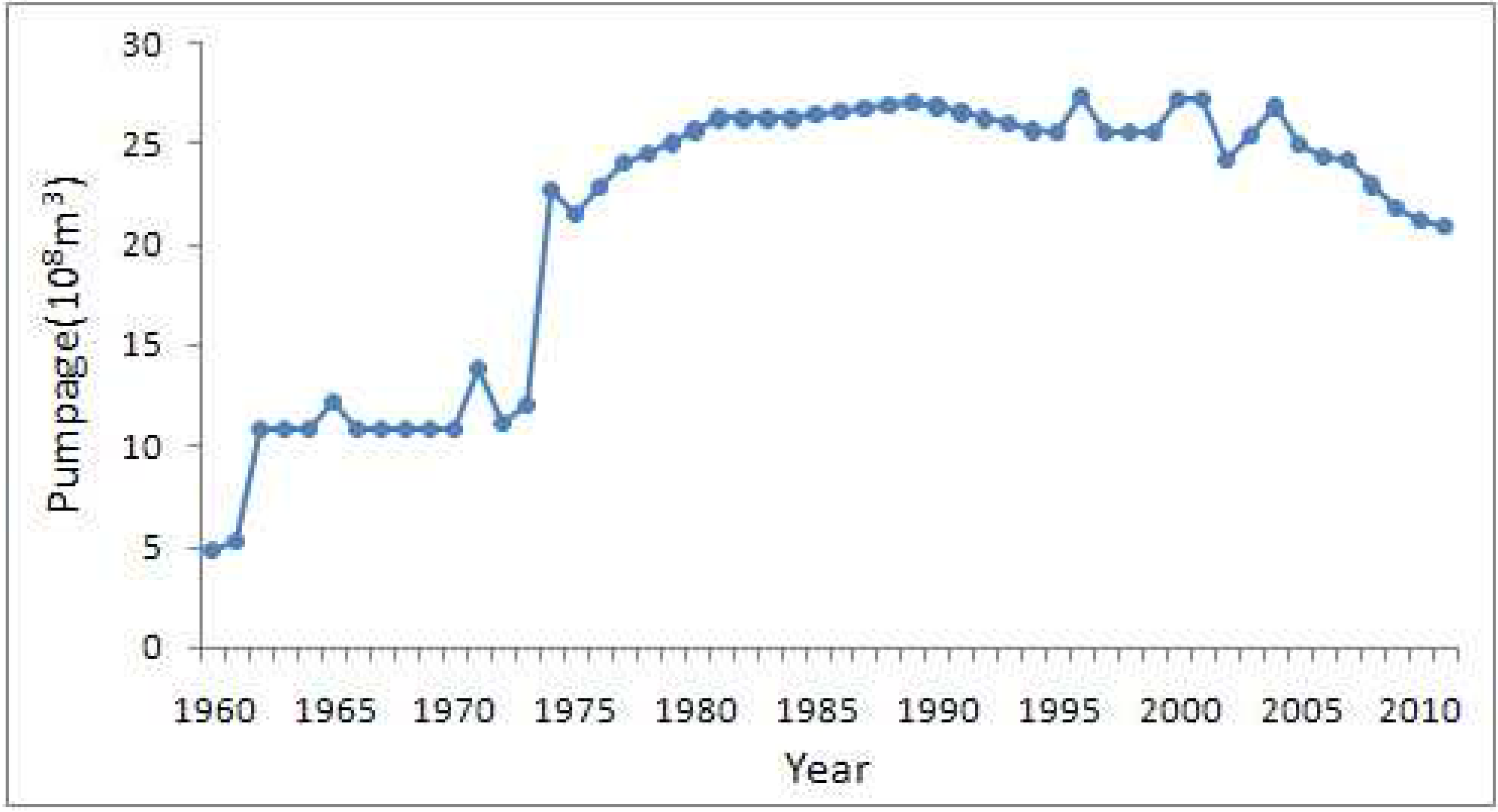
Using the Neural Network Algorithm mentioned in Section 2.1, we can complete pumpage data set (shown in Figure 6), which can be used later in our numerical model.

Table 3. Summary of data collected from 1994 to 2011 for Beijing.

Year	Population (${\mathbf{10}}^{\mathbf{4}}$ persons)	Industrial Output Value (${\mathbf{10}}^{\mathbf{8}}$ CNY)	Grain (${\mathbf{10}}^{\mathbf{4}}$ tons)	Vegetable (${\mathbf{10}}^{\mathbf{4}}$ tons)	Fruits (${\mathbf{10}}^{\mathbf{4}}$ tons)	Irrigated Area (${\mathbf{10}}^{\mathbf{3}}$ hectares)	Pumpage (${\mathbf{10}}^{\mathbf{8}}$ ${\mathbf{m}}^{\mathbf{3}}$)
1994	1,125.0	1,576.6	249.2	350.0	47.2	323.4
1995	1,251.1	1,493.3	259.8	397.3	45.2	292.4	25.5
1996	1,259.4	1,590.6	237.4	403.2	49.5	301.9	27.3
1997	1,240.0	1,819.7	237.5	408.8	52.9	323.3	25.5
1998	1,245.6	1,947.0	239.3	403.8	57.5	323.7	25.5
1999	1,257.2	2,183.5	201.0	419.8	57.8	322.1	25.5
2000	1,363.6	2,842.0	144.2	466.3	63.7	322.7	27.2
2001	1,385.1	3,270.1	104.9	491.0	68.8	322.7	27.2
2002	1,423.2	3,620.2	82.3	507.4	75.6	219.7	24.2
2003	1,456.4	4,410.8	58.0	486.7	80.5	178.9	25.4
2004	1,492.7	5,733.3	70.2	444.1	86.9	186.7	26.8
2005	1,538.0	6,946.2	94.9	373.1	89.6	181.5	24.9
2006	1,581.0	8,210.0	109.2	341.2	84.4	181.5	24.3
2007	1,633.0	9,648.4	102.1	340.1	86.4	173.6	24.2
2008	1,695.0	10,413.1	125.5	321.3	85.1	172.0	22.9
2009	1,755.0	11,039.1	124.8	320.3	120.1	218.7	21.8
2010	1,962.0	13,699.8	115.7	290.8	115.2	211.4	21.2
2011	2,019.0	14,513.6	121.8	293.3	120.9	209.3	20.9

Table 3. Summary of data collected from 1994 to 2011 for Beijing.

Year	Population (${\mathbf{10}}^{\mathbf{4}}$ persons)	Industrial Output Value (${\mathbf{10}}^{\mathbf{8}}$ CNY)	Grain (${\mathbf{10}}^{\mathbf{4}}$ tons)	Vegetable (${\mathbf{10}}^{\mathbf{4}}$ tons)	Fruits (${\mathbf{10}}^{\mathbf{4}}$ tons)	Irrigated Area (${\mathbf{10}}^{\mathbf{3}}$ hectares)	Pumpage (${\mathbf{10}}^{\mathbf{8}}$ ${\mathbf{m}}^{\mathbf{3}}$)
1994	1,125.0	1,576.6	249.2	350.0	47.2	323.4
1995	1,251.1	1,493.3	259.8	397.3	45.2	292.4	25.5
1996	1,259.4	1,590.6	237.4	403.2	49.5	301.9	27.3
1997	1,240.0	1,819.7	237.5	408.8	52.9	323.3	25.5
1998	1,245.6	1,947.0	239.3	403.8	57.5	323.7	25.5
1999	1,257.2	2,183.5	201.0	419.8	57.8	322.1	25.5
2000	1,363.6	2,842.0	144.2	466.3	63.7	322.7	27.2
2001	1,385.1	3,270.1	104.9	491.0	68.8	322.7	27.2
2002	1,423.2	3,620.2	82.3	507.4	75.6	219.7	24.2
2003	1,456.4	4,410.8	58.0	486.7	80.5	178.9	25.4
2004	1,492.7	5,733.3	70.2	444.1	86.9	186.7	26.8
2005	1,538.0	6,946.2	94.9	373.1	89.6	181.5	24.9
2006	1,581.0	8,210.0	109.2	341.2	84.4	181.5	24.3
2007	1,633.0	9,648.4	102.1	340.1	86.4	173.6	24.2
2008	1,695.0	10,413.1	125.5	321.3	85.1	172.0	22.9
2009	1,755.0	11,039.1	124.8	320.3	120.1	218.7	21.8
2010	1,962.0	13,699.8	115.7	290.8	115.2	211.4	21.2
2011	2,019.0	14,513.6	121.8	293.3	120.9	209.3	20.9

Figure 6. Pumpage data for Beijing after restoration.

Figure 6. Pumpage data for Beijing after restoration.

3.5. Model Calibration

The main hydrogeological parameters are hydraulic conductivity, specific yield and specific storage, infiltration coefficient of precipitation, and return leakage coefficient of irrigation water. Within the study area, according to the hydrogeological condition and lithologic characteristics of aquifers, the initial values of these main parameters were defined in different zones, which were regarded as homogeneous within each sub-region [38].

All these hydrogeological parameters can be calibrated by the simulated annealing method mentioned in Section 2.2, which was used to minimize the root-mean-square error (RMSE) between the simulated and observed data. The observed data that were involved in the calibration process included historic water level contour maps in 1975, 1984, 1992, 2003 and 2005 [38,44] and monitoring water level time series between 2003 and 2008 in the observation wells in Figure 5.

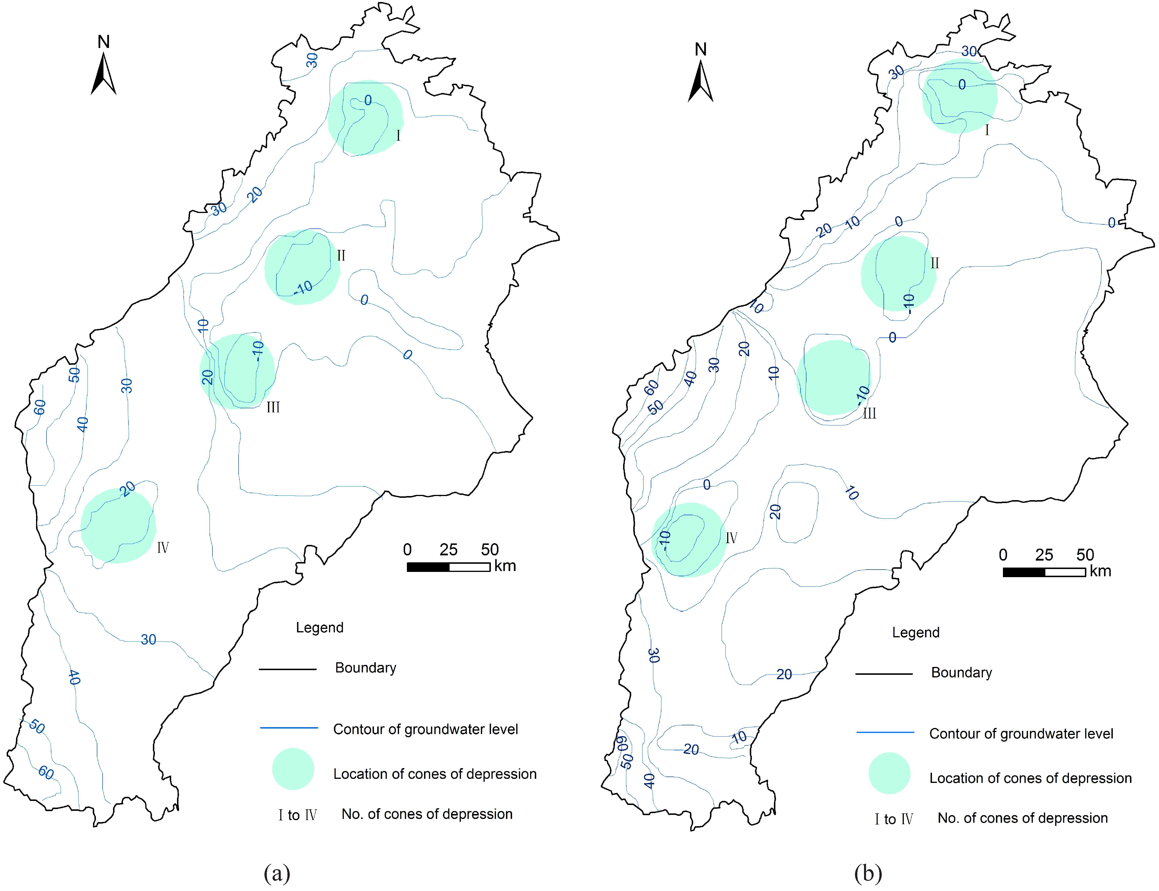
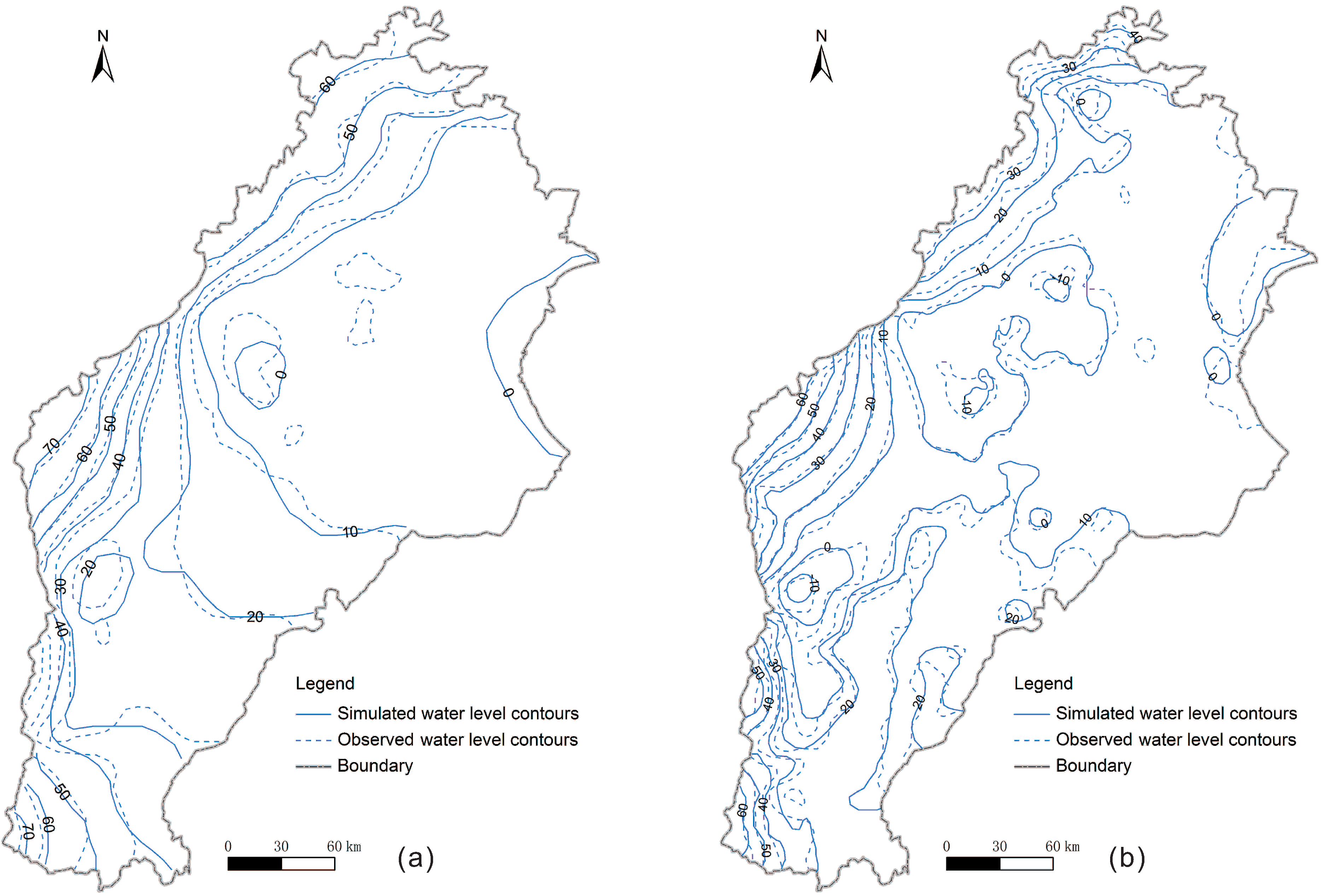
Figure 7 shows that the simulated water level contours are similar to the regional flow pattern of hand-contoured measured water level for 1984 and 2003. The mean error (ME) between simulated and measured water level is 2.74 m, and RMSE is 6.33 m for 142 shallow observation wells (in model layer 1). The ME and RMSE are −2.67 m and 15.73 m, respectively, for 97 deep observation wells (in model layers 2 and 3). These errors are small relative to the maximum groundwater level variations of 60 m [45] and 90 m [46] in the shallow and deep aquifer zones, respectively. Therefore, the model calibration is considered reasonably reliable.

Figure 7. Comparison of observed and simulated water level contours in the shallow aquifer zone in (a) 1984 and (b) 2003.

Figure 7. Comparison of observed and simulated water level contours in the shallow aquifer zone in (a) 1984 and (b) 2003.

4. Results and Discussion

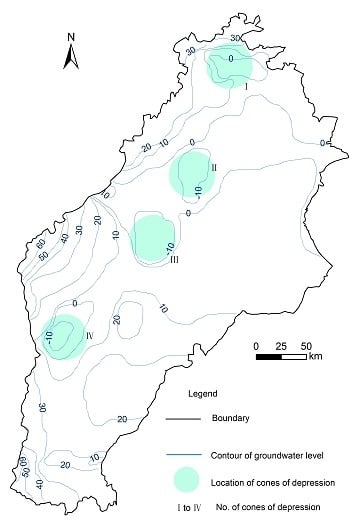
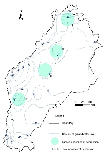
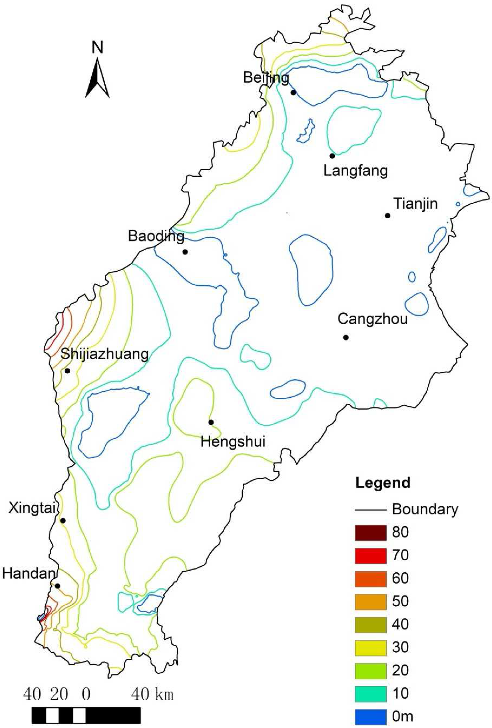
From the results of simulation, we can see that most of the cones of depression in shallow aquifers in the NCP were located in the piedmont clinoplains and the western part of the flood plain, where most of the groundwater supply is from the shallow aquifers [10]. Immense cones of depression were located in Beijing, Langfang, Baoding and Xingtai, most of which were formed in the middle 1970s. Cones of depression in these four places did not appear in the NCP in 1959 (Figure 8). In early 1960s, the depth of groundwater table was near the ground surface [47]. However, they were noticeable in 1985 (Figure 9a), and further expanded in 2005 (Figure 9b).

Figure 8. The contour map of groundwater level in the NCP in 1959 [38].

Figure 8. The contour map of groundwater level in the NCP in 1959 [38].

4.1. Cone of Depression in Beijing

The Beijing Cone of depression was formed in the middle 1970s, and was approximately 250 $k{m}^2$ in 1975 [48]. The shape and location of the cone is shown as No. I in Figure 9. The variation of depth of the cone’s center is shown in Figure 10a. Compared with the groundwater level in 1959 (Figure 8), the groundwater table level depletion is more than 10 m in 1985. The 0 m contour of the cone had a trap area of 630 $k{m}^2$ in 1985. It rapidly increased to 740 $k{m}^2$ in 1996 [48]. However, in 1998, it shrank by 95.5 $k{m}^2$ and the center of it was 31.4 m in depth, which was 0.72 m higher than that in 1997 [46]. In 2005, the 0 m contour of it had a trap area of 934 $k{m}^2$ (Figure 3 and Figure 9b). Because some water conservation measures, such as water saving policies, recycled water utilization, drip irrigation and sprinkler irrigation in agriculture, were taken by the Beijing government, the pumpage began to decline after 2005. However, the Beijing Cone kept expanding. From the year 2005 to 2010 (Figure 10a), the groundwater level at the center of it lowered by 1.29 m/yr on average and finally became 51.47 m in depth in 2010 [46,48].

Figure 9. The contour map of groundwater level in the NCP (a) in 1985; (b) in 2005.

Figure 9. The contour map of groundwater level in the NCP (a) in 1985; (b) in 2005.

Figure 10. Variation of calculated depth of the center of (a) Beijing Cone and (b) Bazhou Cone.

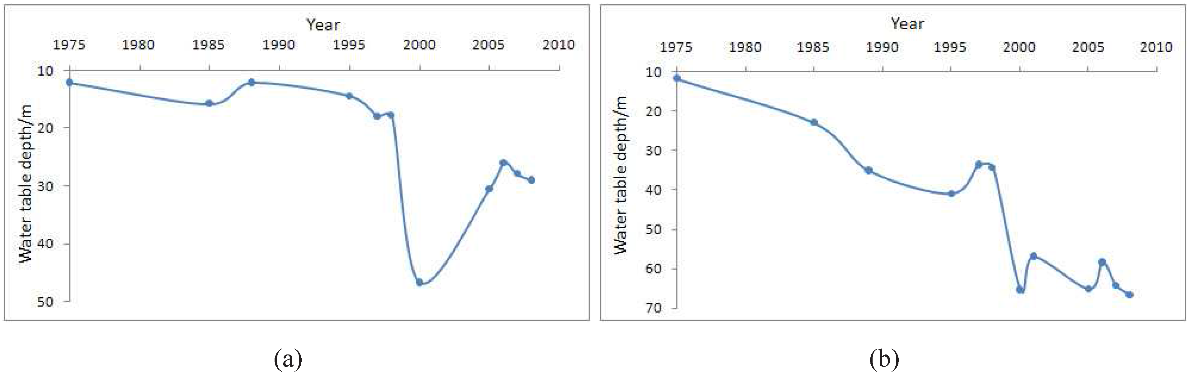
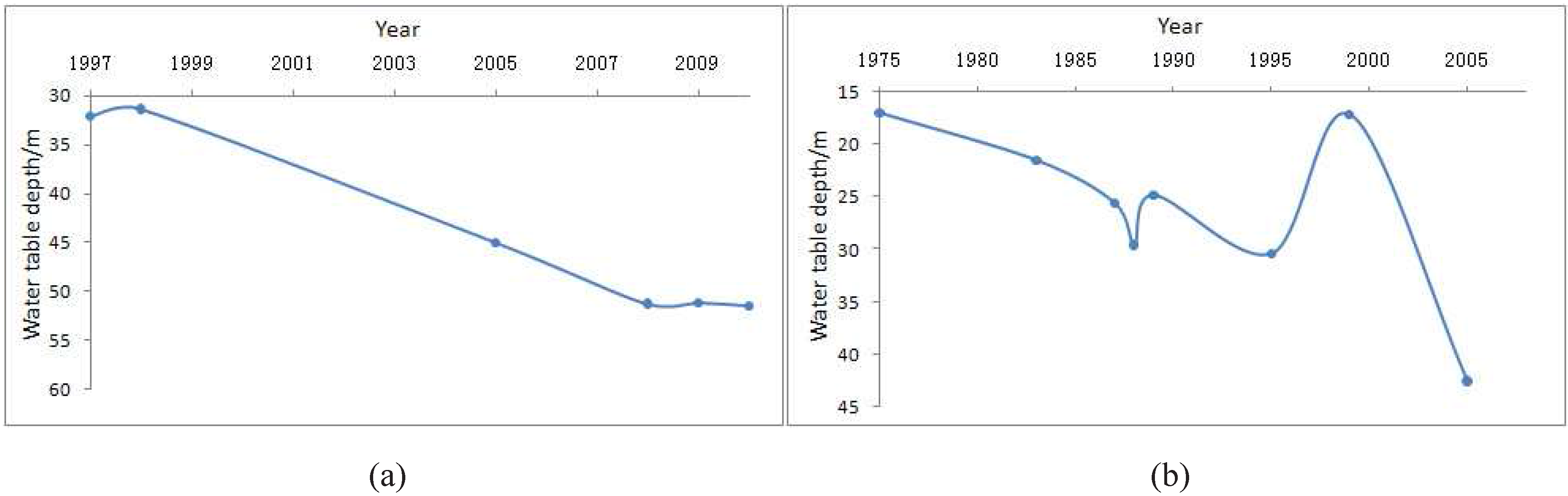
Figure 10. Variation of calculated depth of the center of (a) Beijing Cone and (b) Bazhou Cone.

4.2. Cone of Depression in Bazhou

The Bazhou Cone of depression was formed in 1983. It lies in the southwest of Langfang (No. II in Figure 3 and Figure 9a). The variation of depth of the cone’s center is shown in Figure 10b. Its appearance was likely due to agricultural development [49]. The groundwater level at the center of it declined by 25.5 m from the year 1975 to 2005 [38]. Compared with the groundwater level in 1959 (Figure 8), the groundwater table level near the cone of depression changed from more than 0 m to less than −10 m in 1985 (Figure 3 and Figure 9b). In 1985, the −10 m contour of it had a trap area of 830 $k{m}^2$. In 1987, the depth of the cone’s center was 25.64 m, and turned to be 30.4 m in 1995 [48,49]. In 2005, the area of the −10 m contour of the cone expanded to 1224 $k{m}^2$ . At present, groundwater resource is still very important for the agriculture in this area. The cone is expanding to the north.

4.3. Cone of Depression in Lixian

The Lixian Cone of depression was formed in 1973. It locates at the boundary between Baoding and Cangzhou (No. III in Figure 3 and Figure 9), where the groundwater is mainly extracted from the first and the second aquifer groups. The variation of depth of the cone’s center is shown in Figure 11a. At the very beginning, the center of the cone is 3 m lower than the boundary of it. However, in 1975, the depth of its center turned to be 12.1 m and went down further by 3.69 m in 1985 as shown in Figure 11a [48]. In 1985, the −10 m contour of it had a trap area of 673 $k{m}^2$. After that, although there was a short recovery for the cone, the groundwater level of its center declined every year right after the short prosperity and it reached the maximum depth at 46.73 m in 2000, which is 28.89 m less than that in 1998 [46,48]. When it came to the year 2005, the groundwater level of its center recovered by more than 15 m [48], and the −10 m contour of it had an area of 1758 $k{m}^2$. In 2006, the groundwater level at the cone’s center climbed up further and reached a local maximum (Figure 11a). However, after that it began to decline again and became 29 m in 2008 [45].

Figure 11. Variation of calculated depth of the center of (a) Lixian Cone and (b) Ningbolong Cone.

Figure 11. Variation of calculated depth of the center of (a) Lixian Cone and (b) Ningbolong Cone.

4.4. Cone of Depression in Ningbolong

The Ningbolong Cone of depression lies at the boundary between Xingtai and Baoding (No. IV in Figure 3 and Figure 9), where the groundwater is mainly extracted from the shallow aquifer groups. It was formed in 1972 [48]. Figure 11(b) shows the variation of depth of the center of the cone among all these years. In 1975, the depth was 11.78 m, while it was almost 22 m in 1985 [48]. In 1985, the 20 m contour of it had a trap area of 1550 $k{m}^2$. In 1989, the center of it located at Baiyang Ying, Bai Xiang, and then transferred to Zhao Zhuang in 1995 [35]. In 2005, the trap area of 20 m contour in 1985 is almost replaced by the trap area of 0 m contour, and the 0 m contour of the cone had an area of 1700 $k{m}^2$ (Figure 9b). In 2008, the depth of its center reached 66.75 m [45].

4.5. Evaluation of the Exploitation Limitation Strategy

Based on projected water allocation plans of the SNWDP [13], the following scenario is simulated: the groundwater exploitation from 2015 to 2020 is reduced by 3.5 billion $m^3$, which is approximately 25% of the groundwater exploitation in 2011. The first phase of the project will be completed after the flood season in 2014, supplying the NCP with 5.7 billion $m^3$ of water annually [50]. Therefore, the reduction is less than the supply from the SNWDP.

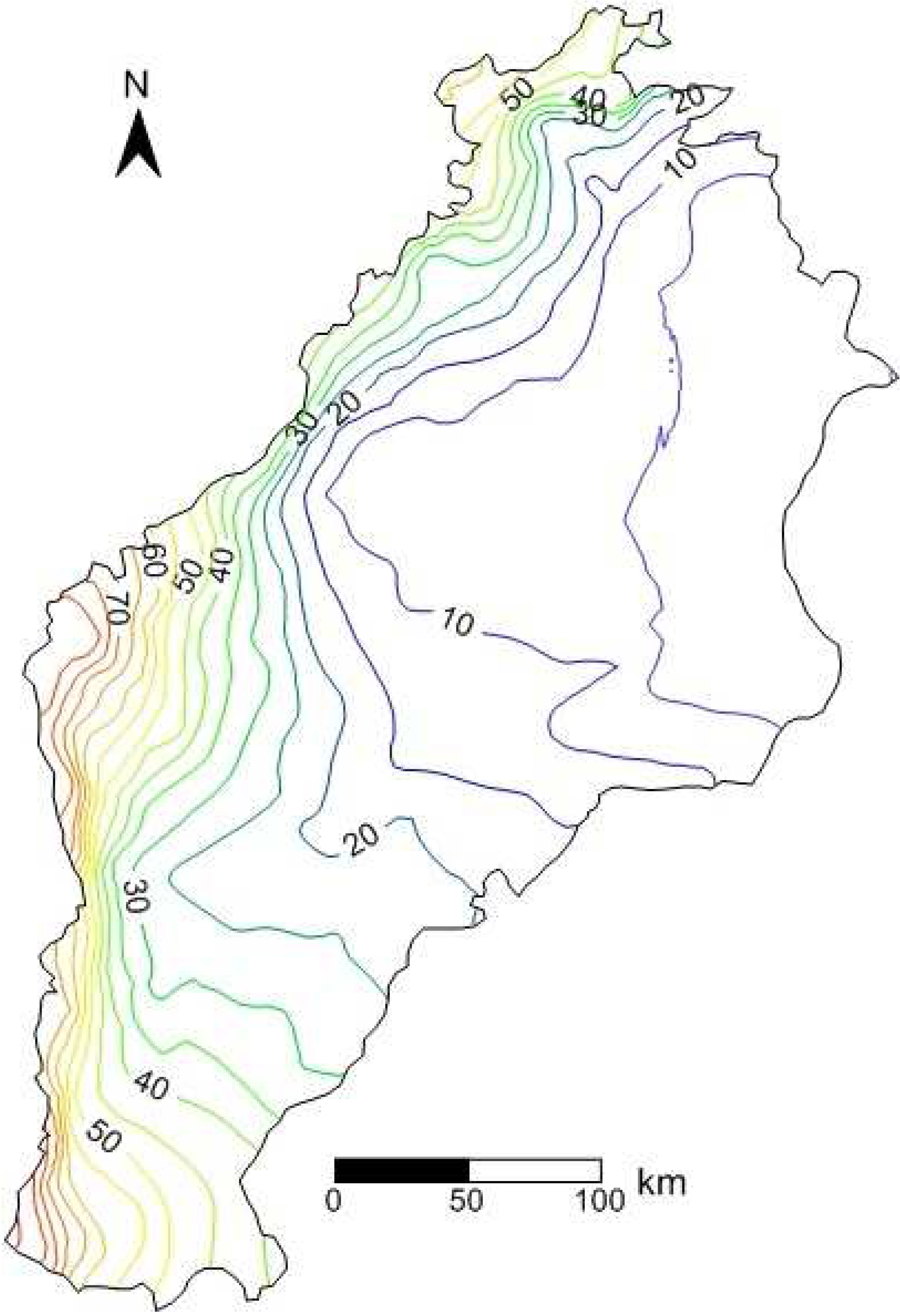
As shown in Figure 12, the groundwater level in shallow aquifers across the whole NCP will rise because of the limitation on groundwater extraction. Moreover, some but not all of the cones of depression will shrink. For example, the area of the cone of depression contained in the 0 m in Bazhou and Lixian is 5825 $k{m}^2$ in 2008, 3559 $k{m}^2$ in 2020. However, the cone of depression in Beijing will continue expanding after the construction of the SNWDP. The area of the 0 m contour of the cone of depression in Beijing will be 2155 $k{m}^2$ in 2020, while it was 1380 $k{m}^2$ in 2008. The area of the 10 m contour of the cone of depression in Beijing will be 991 $k{m}^2$ in 2020, while it was 840 $k{m}^2$ in 2008. This finding implies that groundwater resource recovery will be more difficult in this area. In summary, the cones of depression will change but cannot thoroughly recover in 2020. Therefore, it will take a long time to the recovery of cones of depression in shallow aquifers after the SNWDP. This result exhibits similar phenomenon with that in Visocky’s work [18], i.e., the major cones will continue to spread outward after the Lake Michigan Allocation if the over-exploitation is not stopped. To strengthen the effect of the SNWDP, other measures should be carried out at the same time, such as agricultural water savings (mentioned in [28]).

Finally, we got an overall understanding about the evolution of cones of depression. We can see that cones of depression in the NCP began to appear in 1970s and anthropogenic activities are the root cause. The SNWDP is beneficial for groundwater recovery in the NCP. A number of immense groundwater cones will gradually shrink. However, the recovery of the groundwater environment in the NCP will require a long time.

Figure 12. The contour map of predicted groundwater level in the NCP in 2020.

Figure 12. The contour map of predicted groundwater level in the NCP in 2020.

5. Conclusions

The cones of depression in the shallow aquifers in the NCP appeared in 1970s. Then, the cones of depression expanded gradually because of the groundwater exploitation in the NCP. To mitigate the shortage of water resources and groundwater depletion in the NCP, the construction of the SNWDP has started and may be completed by 2014. In this paper, the hydrogeological conditions and geological structure of the NCP were systematically analyzed. To show the past and future recovery of the cones of depression in the NCP, a 3D transient groundwater flow numerical model was built. The model was run under drought climate conditions with the limited extraction stages to predict the groundwater dynamic changes after the construction of the SNWDP.

The conclusions are as follows:

(1) Most of the cones of depression in shallow aquifers in the NCP lie in the piedmont clinoplains and the flood plain. The cones of depression located in Beijing, Langfang, Baoding and Xingtai were expanding over the last 40 years. The groundwater levels at the center of the cones of depression declined every year before 1990 and oscillated after 1990. The overexploitation of groundwater in the NCP lasted for more than thirty years, although the level of overexploitation varied with development demands and climate changes. Anthropogenic activities, including construction of the dams, urban water supply and agricultural irrigation, were the main reason for the formation of the cones.

(2) The SNWDP will significantly mitigate water shortage and the deterioration of the groundwater system in the NCP. The limited exploitation of groundwater can remediate groundwater cones to a certain extent, but an extended period of time is necessary for the recovery of the groundwater environment because of the overpumping in the past in the NCP.

(3) From the prediction, we can see that Beijing Cone continues expanding even after the implementation of SNWDP. Therefore, more exploitation limitation measures are needed to be carried out in this region and more water should be transferred to Beijing to stop the expansion of cones of depression.

References

- De Vries, J.J.; Simmers, I. Groundwater recharge: An overview of processes and challenges. Hydrogeol. J. 2002, 10, 5–17. [Google Scholar] [CrossRef]
- Wada, Y.; van Beek, L.P.H.; van Kempen, C.M.; Reckman, J.W.T.M.; Vasak, S.; Bierkens, M.F.P. Global depletion of groundwater resources. Geophys. Res. Lett. 2010, 37, L20402. [Google Scholar] [CrossRef]
- Custodio, E. Aquifer overexploitation: What does it mean? Hydrogeol. J. 2002, 10, 254–277. [Google Scholar] [CrossRef]
- Almedeij, J.; Al-Ruwaih, F. Periodic behavior of groundwater level fluctuations in residential areas. J. Hydrol. 2006, 328, 677–684. [Google Scholar] [CrossRef]
- La Vigna, F.; Mazza, R.; Capelli, G. Detecting the flow relationships between deep and shallow aquifers in an exploited groundwater system, using long-term monitoring data and quantitative hydrogeology: The Acque Albule Basin case (Rome, Italy). Hydrol. Process. 2012. [Google Scholar] [CrossRef]
- Michael, H.A.; Voss, C.I. Controls on groundwater flow in the Bengal Basin of India and Bangladesh: Regional modeling analysis. Hydrogeol. J. 2009, 17, 1561–1577. [Google Scholar] [CrossRef]
- Jia, J.S.; Liu, C.M. Groundwater dynamic drift and response to different exploitation in the North China Plain: A case study of luancheng county, Hebei Province [in Chinese]. Acta Geogr. Sin. 2002, 57, 201–209. [Google Scholar]
- Sun, X.B.; Sun, H.; Zhai, P.Y.; Dong, X.D. Study on formation mechanism of cones of depression [in Chinese]. Ground Water 2012, 34, 29–30. [Google Scholar]
- Li, Y.S.; Fei, Y.H.; Qian, Y.; Jian, M.; Han, Z.T.; Wang, P.; Zhang, Z.J. Discussion on evolution characteristics and formation mechanism of deep groundwater depression cone in Cangzhou region [in Chinese]. J. Arid Land Resour. Environ. 2013, 27, 181–184. [Google Scholar]
- Fei, J. Groundwater resources in the North China Plain. Environ. Geol. Water Sci. 1988, 12, 63–67. [Google Scholar] [CrossRef]
- Cao, G.L.; Zheng, C.M.; Scanlon, B.R.; Liu, J.; Li, W.P. Use of flow modeling to assess sustainability of groundwater resources in the North China Plain. Water Resour. Res. 2013, 49, 1–17. [Google Scholar] [CrossRef]
- Fei, Y.H.; Miao, J.X.; Zhang, Z.J.; Chen, Z.Y.; Song, H.B.; Yang, M. Analysis on evolution of groundwater depression cones and its leading factors in North China Plain [in Chinese]. Resour. Sci. 2009, 31, 394–399. [Google Scholar]
- Liu, C.M.; Zheng, H.X. South-to-North water transfer schemes for China. Water Res. Dev. 2002, 18, 453–471. [Google Scholar] [CrossRef]
- General program of the South-to-North water transfer project. China Water Resour. 2003, 1B, 3–6.
- Nakayama, T.; Yang, Y.; Watanabe, M.; Zhang, X.Y. Simulation of groundwater dynamics in the North China Plain by coupled hydrology and agricultural models. Hydrol. Processes 2006, 20, 3441–3466. [Google Scholar] [CrossRef]
- Kirk, R.W.; Bolstad, P.V.; Manson, S.M. Spatio-temporal trend analysis of long-term development patterns (1900–2030) in a southern appalachian county. Landsc. Urban Plan 2012, 104, 47–58. [Google Scholar] [CrossRef]
- Ajami, H. RIPGIS-NET: A GIS tool for riparian groundwater evapotranspiration in MODFLOW. Ground Water 2012, 50, 47–58. [Google Scholar] [CrossRef] [PubMed]
- Visocky, A.P. Impact of lake Michigan allocations on the Cambrian-Ordovician aquifer system. Ground Water 1982, 20, 668–674. [Google Scholar] [CrossRef]
- Rubio, S.J.; Casino, B. Competitive versus efficient extraction of a common property resource: The groundwater case. J. Econ. Dyn. Control 2001, 25, 1117–1137. [Google Scholar] [CrossRef]
- Lin, L.; Yang, J.Z.; Zhang, B.; Zhu, Y. A simplified numerical model of 3-D groundwater and solute transport at large scale area. J. Hydrodyn. 2010, 22, 319–328. [Google Scholar] [CrossRef]
- Feng, S.; Li, L.X.; Duan, Z.G.; Zhang, J.L. Assessing the impacts of South-to-North water transfer project with decision support systems. Decis. Support Syst. 2007, 42, 1989–2003. [Google Scholar] [CrossRef]
- Liu, J.; Zheng, C.; Lei, Y. Ground water sustainability: Methodology and application to the North China Plain. Ground Water 2008, 46, 897–909. [Google Scholar] [CrossRef] [PubMed]
- Hu, Y.K.; Moiwo, J.P.; Yang, Y.H.; Han, S.M.; Yang, Y.M. Agricultural water-saving and sustainable groundwater management in Shijiazhuang irrigation district, North China Plain. J. Hydrol. 2010, 393, 219–232. [Google Scholar] [CrossRef]
- Yang, Y.; Li, G.M.; Dong, Y.H.; Li, M.; Yang, J.Q.; Zhou, D.; Yang, Z.S.; Zheng, F.D. Influence of south to north water transfer on groundwater dynamic change in Beijing plain. Environ. Earth Sci. 2012, 65, 1323–1331. [Google Scholar] [CrossRef]
- Zhang, Z.H.; Shi, D.H.; Ren, F.H.; Yin, Z.Z.; Sun, J.C.; Zhang, C.Y. Evolution of quaternary groundwater system in North China Plain. Sci. China Ser. D 1997, 3, 276–283. [Google Scholar] [CrossRef]
- Wang, S.Q.; Shao, J.L.; Song, X.F.; Zhang, Y.B.; Huo, Z.B.; Zhou, X.Y. Application of MODFLOW and geographic information system to groundwater flow simulation in North China Plain, China. Environ. Geol. 2008, 55, 1449–1462. [Google Scholar] [CrossRef]
- Cui, Y.L.; Wang, Y.; Shao, J.; Chi, Y.; Lin, L. Research on groundwater regulation and recovery in North China Plain after the implementation of South-to-North water transfer [in Chinese]. Resour. Sci. 2009, 31, 382–387. [Google Scholar]
- Foster, S.; Gardumo, H.; Evans, R.; Olson, D.; Tian, Y.; Zhang, W.Z.; Han, Z.S. Quaternary aquifer of the North China Plain–Assessing and achieving groundwater resource sustainability. Hydrogeol. J. 2004, 12, 81–93. [Google Scholar] [CrossRef]
- Aji, K.; Tang, C.; Song, X.; Kondoh, A.; Sakura, Y.; Yu, J.; Kaneko, S. Characteristics of chemistry and stable isotopes in groundwater of Chaobai and Yongding River basin, North China plain. Hydrol. Process. 2008, 22, 63–72. [Google Scholar] [CrossRef]
- Rumelhart, D.E.; McClelland, J.L. Parallel Distributed Processing: Explorations Inthe Microstructure of Cognition; MIT Press: Cambridge, MA, USA, 1986; pp. 318–362. [Google Scholar]
- Li, Z.H.; Wang, Y.F.; Yang, C.C. A fast global optimization algorithm for regularized migration imaging. Chin. J. Geophys. 2011, 54, 828–834. [Google Scholar] [CrossRef]
- Wang, X.Y.; Chen, J.; Sun, L.; Han, S.P.; Fei, Y.H.; Wang, J.S.; Liu, C.L.; Zhang, Y. Laboratory study on the relationship between soil mass deformation and water seepage in North China. Environ. Earth Sci. 2011, 64, 2195–2201. [Google Scholar] [CrossRef]
- Wang, L.S.; Ma, C. A study on the environmental geology of the middle route project of the South-North water transfer. Eng. Geol. 1999, 51, 153–165. [Google Scholar] [CrossRef]
- Zhang, Z.J.; Luo, G.Z.; Wang, Z.; Liu, C.M.; Li, T.S.; Jiang, X.Q. Study on sustainable utilization of groundwater in North China Plain [in Chinese]. Resour. Sci. 2009, 3, 355–360. [Google Scholar]
- Chen, W.H. Groudwater in Hebei Province [in Chinese]; Seismological Press: Beijing, China, 1999. [Google Scholar]
- McDonald, M.G.; Harbaugh, A.W. A Modular Three-Dimensional Finite Diffe Rence Groundwater Flow Model. In Techniques of Water-Resources Investigations of the USGS; U.S. Geological Survey: Reston, VA, USA, 1988. [Google Scholar]
- Harbaugh, A.W.; Banta, E.R.; Hill, M.C.; McDonald, M.G. MODFLOW-2000, The U.S. Geological Survey Modular Ground-Water Model User Guide to Modularization Concepts and the Ground-Water Flow Process; U.S. Geological Survey: Reston, VA, USA, 2000. [Google Scholar]
- Zhang, Z.J.; Fei, Y.H. Atlas of Groundwater Sustainable Utilization in NorthChina Plain [in Chinese]; Zhang, Z.J., Fei, Y.H., Eds.; Sinomaps Press: Beijing, China, 2009. [Google Scholar]
- Wang, S.Q.; Song, X.F.; Wang, Q.X.; Xiao, G.Q.; Liu, C.M.; Liu, J.R. Shallow groundwater dynamics in North China Plain. J. Geogr. Sci. 2009, 19, 175–188. [Google Scholar] [CrossRef]
- Chung, I.M.; Kim, N.W.; Lee, J.; Sophocleous, M. Assessing distributed groundwater recharge rate using integrated surfacewater–groundwater modeling: Application to Mihocheon watershed. S. KoreaI1 Moon. Hydrogeol. J. 2010, 18, 1253–1264. [Google Scholar] [CrossRef]
- Susan, K.J. Applications of hydrologic information automatically extracted from digital elevation models. Hydrol. Process. 1991, 5, 31–44. [Google Scholar] [CrossRef]
- Xu, H.Z. Study on Numerical Simulating Methods for Delineation of Groundwaterresource Protection Area [in Chinese]; Dissertation, The China Academy of Science: Beijing, China, 2011. [Google Scholar]
- National Bureau of Statistics of China, 2003; Annual Data. Available online: http://www.stats.gov.cn/english/statisticaldata/yearlydata/ (accessed on 7 April 2013).
- Zhang, Z.H.; Shen, Z.L.; Xue, Y.Q.; Ren, F. Groundwater Environment Evolution in the North China Plain [in Chinese]; Geological Publishing House: Beijing, China, 2000. [Google Scholar]
- Hebei Water, People’s Government of Hebei Province, 2013. In Groundwater Bullitin 2008. Available online: http://www.hebwater.gov.cn/ (accessed on 7 April 2013).
- Haihe River Water Conservancy Commission, 2013. Haihe River Water Resources Bulletin 1998–2010. Available online: http://www.chinawater.net.cn (accessed on 7 April 2013).
- Tamanyu, S.; Muraoka, H.; Ishii, T. Geological interpretation of groundwater level lowering in the North China Plain. S. Bull. Geol. Surv. Jpn. 2009, 60, 105–115. [Google Scholar] [CrossRef]
- Zhang, Z.J. Investigation and Evaluation of Sustainable Utilization of Groundwater in North China Plain [in Chinese]; Geological Publishing House: Beijing, China, 2009. [Google Scholar]
- He, P. Analysis ongroundwater overdraft status and its countermeasure in Langfang City [in Chinese]. Ground Water 2009, 31, 59–61. [Google Scholar]
- Changjiang Water Resources Commission of the Ministry of Water Resources. The South-to-North water transfer project planning (2001 revision) [in Chinese]. China Water Resour. 2003, 1B, 48–55. [Google Scholar]
© 2013 by the authors; licensee MDPI, Basel, Switzerland. This article is an open access article distributed under the terms and conditions of the Creative Commons Attribution license (http://creativecommons.org/licenses/by/3.0/).
Share and Cite
MDPI and ACS Style
Zhang, Y.; Li, G. Long-Term Evolution of Cones of Depression in Shallow Aquifers in the North China Plain. Water 2013, 5, 677-697. https://doi.org/10.3390/w5020677
AMA Style
Zhang Y, Li G. Long-Term Evolution of Cones of Depression in Shallow Aquifers in the North China Plain. Water. 2013; 5(2):677-697. https://doi.org/10.3390/w5020677
Chicago/Turabian StyleZhang, Yuan, and Guomin Li. 2013. "Long-Term Evolution of Cones of Depression in Shallow Aquifers in the North China Plain" Water 5, no. 2: 677-697. https://doi.org/10.3390/w5020677