Article

Bankfull Hydraulic Geometry Relationships for the Inner and Outer Bluegrass Regions of Kentucky

1
Biosystems and Agricultural Engineering Department, University of Kentucky, 128 C.E. Barnhart Building, Lexington, KY 40502, USA
2
Assistant Dean for Research and Associate Director of the Agricultural Experiment Station, University of Kentucky, S-129 Agriculture Science Center North, Lexington, KY 40546, USA
3
Civil Engineering Department, University of Kentucky, 354F Oliver Raymond Building, Lexington, Kentucky 40546, USA
4
Kentucky Geological Survey, Biosystems and Agricultural Engineering Department, University of Kentucky, 228 Mining and Minerals Resource Building, Lexington, KY 40546, USA
*
Author to whom correspondence should be addressed.
Water 2011, 3(3), 923-948; https://doi.org/10.3390/w3030923
Submission received: 27 June 2011 / Revised: 27 August 2011 / Accepted: 9 September 2011 / Published: 20 September 2011

Abstract

:
Bankfull hydraulic geometry relationships relate bankfull stream dimensions, such as cross-sectional area, width, mean depth, mean velocity, width to depth ratio, and slope to bankfull discharge. These relationships can assist in determining a design discharge for stream restoration and management projects. This study assessed 27 stable streams located in the Inner Bluegrass and Outer Bluegrass regions of Kentucky. Reaches were selected based on the presence of a U.S. Geological Survey gage, as well as other conditions such as presence of readily identifiable bankfull indicators, stability indices, and site accessibility. Bankfull channel dimensions and discharges were determined, and hydraulic geometry relationships were developed for both the Inner Bluegrass and Outer Bluegrass regions. These scaling relationships for karst-influenced streams were similar to others reported in the literature for non-karst areas. Significant differences between the regions were found only for bankfull width and width-to-depth ratio. Streams in the Inner Bluegrass tended to be more narrow and deep at bankfull discharges less than 10 m3s−1 and wider and shallower at bankfull discharges greater than 20 m3s−1 as compared to stream in the Outer Bluegrass. It is suspected that physiographic conditions related to local geology and/or riparian vegetation at three sites in the Outer Bluegrass accounted for these differences. Results of this study indicate that in instances of geologic variation within a physiographic region, hydraulic geometry relationships may require evaluation at the watershed scale.

Graphical Abstract

1. Introduction

Hydraulic geometry provides a means for enhancing our ability to assess and design stream projects [1,2,3]. Hydraulic geometry equations describe the relationship between a stream’s form, such as cross-sectional area, width, mean depth, mean velocity, and slope, and a single representative discharge such as bankfull discharge [3,4,5,6]. Bankfull discharge is the discharge at which the stream flows at the top of its banks just before waters spill onto the floodplain [6,7,8,9]. Bankfull discharge is a deterministic discharge often used to estimate the channel-forming discharge [6]. As defined by Copeland et al. [6], the channel-forming discharge is a single discharge that over a long period of time would theoretically “produce the same channel geometry as the natural long-term hydrograph.” While Copeland et al. [6] referred to stable alluvial channels, Fola and Rennie [10] noted that the concept of channel forming discharge is applicable to non-alluvial channels. In addition to bankfull discharge, channel forming discharge can also be estimated by computing effective discharge, which is the discharge that transports the maximum annual sediment load [6,11,12,13,14,15]. Both Andrews [8] and Andrews and Nankervis [16] found that effective discharge and bankfull discharge were equivalent for streams in the western U.S. However, the difficulty with using effective discharge as a means to estimate channel-forming discharge is that a large amount of data is required as both flow duration and sediment rating curves are needed. This data requirement makes the computation of effective discharge impractical in many situations. Annable et al. [17] noted that the sediment rating curves used to compute effective discharge are typically created using only suspended sediment data. By not including bed load data, which is often difficult to acquire, the authors state that such effective discharge computations may contain significant error, particularly when considering coarse-bed systems such as gravel channels.
The physical characteristics of natural streams are interconnected [18]. Leopold and Maddock [4] recognized this and used empirical data collected over a 70-year period to develop hydraulic geometry equations using a single representative discharge, Q, which was the mean annual discharge.
The equations are as follows:
w = aQb
d = cQf
v = kQm
The variables w, d, and v are the parameters width, mean depth, and mean velocity, respectively. The coefficients or intercepts are represented by a, c, and k. The exponents or slopes are represented by b, f, and m. Based on the continuity equation where Q = (w)(d)(v), the product of the respective coefficients (a)(c)(k) equals one, and the sum of the exponents (b + f + m) equals one [5]. Hydraulic geometry relationships can be developed for a single cross-section, termed at-a-station, where changes in channel form at a single location are examined in relation to changes in discharge. Such relationships can also be developed in the downstream direction along a stream network for a specific discharge such as bankfull discharge. In general, the bankfull discharge will increase in the downstream direction since runoff is contributed from larger drainage areas [15].
The hydraulic geometry equations developed by Leopold and Maddock [4] assume steady, uniform flow conditions meaning the water surface slope is parallel with the energy grade line [5]. Because of this assumption, the mean values of the variables used in the general hydraulic geometry relationships must correspond to the equilibrium state of the channel [3]. Equilibrium in a stream involves the interaction of sediment discharge, sediment particle size, stream flow, and stream slope, and is achieved when all four independent variables are in balance [19]. Lane [19] showed the relationship as:
Q s · D 50 Q w · S
where QS refers to the sediment discharge, D50 refers to the median sediment particle size, QW refers to the stream flow, and S refers to the slope. Leopold et al. [5] noted that an alluvial stream in equilibrium has both properties of adjustability and stability. Such a “graded’ stream [20] is one in which the slope is adjusted to provide the velocity required to transport the sediment load provided by the watershed, given discharge and channel characteristics. If one of the variables in (4) changes, the other variables will either increase or decrease to maintain a state of equilibrium. For example, if QW increases, either the QS or D50 or both must also increase to maintain equilibrium in the channel. Leopold and Maddock [4] and Wolman [21] found that a stream adjusts its hydraulic geometry to carry its sediment load to reach a state of equilibrium. Pietsch and Nanson [22] state that a stream will adjust its shape to accommodate changes in discharge in a nonlinear manner with a greater response occurring in the parameter width followed by mean depth and then mean velocity. Since each stream has different boundary conditions (e.g., stream bank material and vegetation), the equilibrium state for each stream differs [3,23]. Knighton [24] found that in the absence of high flows, channels can adjust their form over a relatively short period of time thus suggesting that the approach to equilibrium is relatively rapid.
As noted by Castro and Jackson [25], a substantial amount of research into hydraulic geometry relationships, both empirical and theoretical [3,4,5,26,27,28,29], has been performed. However, research regarding hydraulic geometry relationships for non-alluvial streams is limited, particularly in comparison to alluvial channels [30]. Fola and Rennie [10] studied clay-dominated cohesive bed rivers in Canada and found that hydraulic geometry concepts could be extended to these non-alluvial systems. Wohl and David [30] evaluated hydraulic geometry relationships for bedrock channels using a dataset comprised of 47 sites located predominately the western U.S. but also including sites in Maryland and a few in West Virginia, as well as the countries of Japan, Australia, Panama, India, and Israel. The authors found that while alluvial streams tended to be slightly wider than bedrock ones, a similar finding by Montgomery and Gran [31], both scaled at similar rates with respect to discharge. Wohl and David [30] concluded that other factors than the erosional resistance types accounted for channel geometry of these two stream types. However, none of these studies occurred in karst-influenced areas. Research regarding hydraulic geometry relationships for karst-influenced streams, such as those in the Bluegrass Region of Kentucky where bedrock streams with cohesive banks are common, is lacking. This project will assist in our understanding of how such streams in karst-influenced geology scale with respect to discharge.
Furthermore, the Inner Bluegrass and Outer Bluegrass regions are areas where the number of stream restoration and management projects is relatively high for the southeastern U.S. [32]. However, information on hydraulic geometry whereby bankfull parameters are regressed on bankfull discharges is not available for the Bluegrass Region. As discharge may be used as one of the independent variables, along with sediment inflow and bed material composition, to compute the design variables width, mean depth, slope and planform [2,33], knowledge of hydraulic geometry relationships can assist the design process, particularly in the initial phases.
The objectives of this study were to (1) develop bankfull hydraulic geometry relationships for the Inner Bluegrass and Outer Bluegrass regions of Kentucky and (2) determine if the relationships differ between the regions. As noted by Johnson and Fecko [34] and Keaton et al. [35], regional relationships are typically developed for each physiographic region as climate, geology, topography and soils influence the morphology of streams. Since the Inner Bluegrass region has more extensive karst geology, lower relief, and different soil types than the Outer Bluegrass region, it is hypothesized the hydraulic geometry relationships between the two regions will differ.

2. Materials and Methods
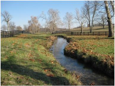
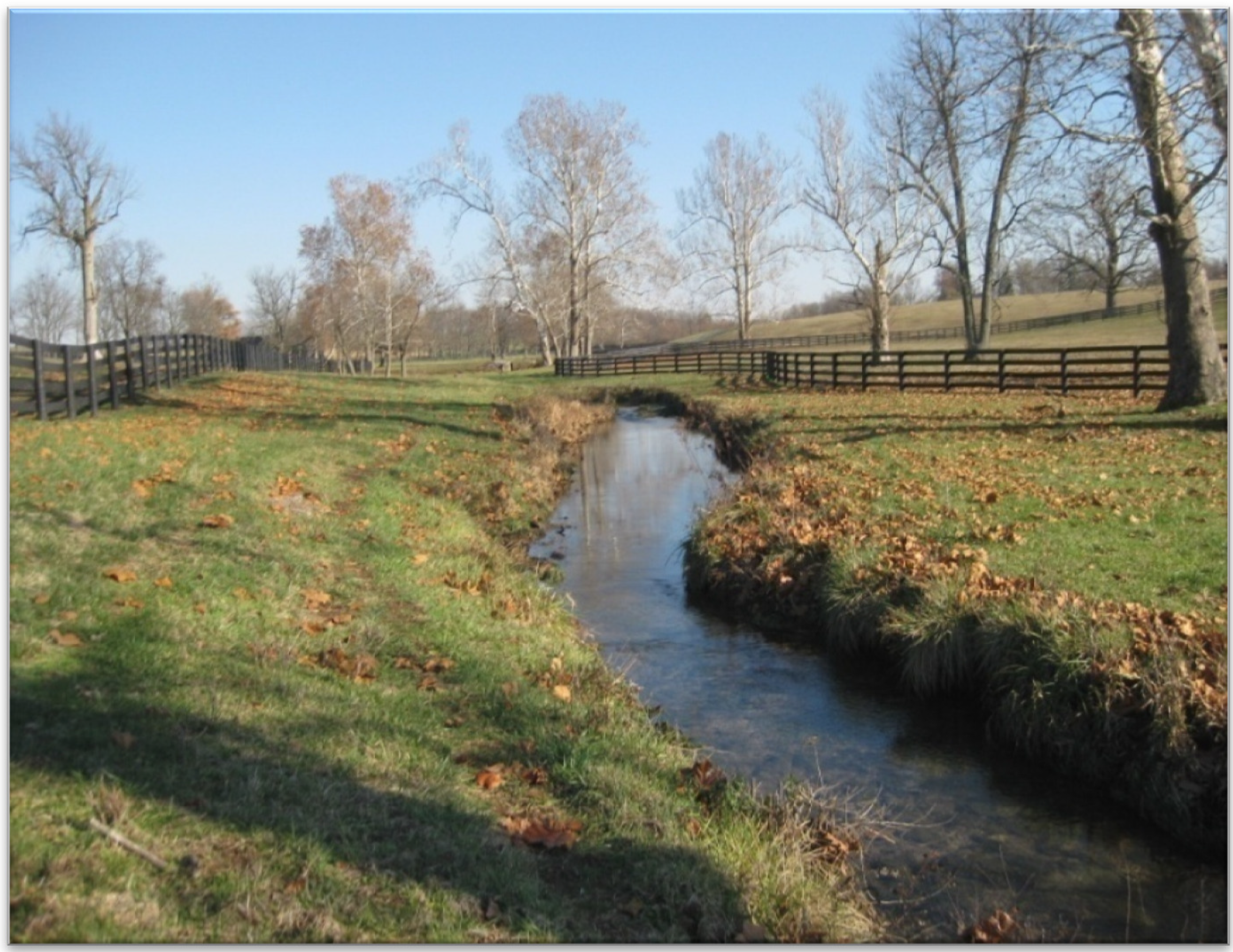
2.1. Study Area

The study was conducted in the Bluegrass Region of Kentucky, USA, which is located in the central and northern portions of the state. The Bluegrass Region is subdivided into the Inner Bluegrass and Outer Bluegrass regions (Figure 1). The Inner Bluegrass is an almost circular region, centered on Lexington, Kentucky (latitude 38.05°N; longitude 85.00°W). This region is about 4,660 km2 in size and is characterized by gently rolling topography, phosphate-rich soils, and extensive karst geology [36,37]. The geology of the Inner Bluegrass is dominated by Lexington Limestone (Ordovician strata) [38]. Weathering of this limestone has produced a large number of sink holes, springs and caves throughout the region [37]. Topography within the region is characterized as having very low relief with typical elevations between 168 m and 326 m above mean sea level [39]. Soils in the Inner Bluegrass have significantly higher permeabilities (15 to 152 mm hr−1) as compared to the Outer Bluegrass (< 15 mm hr−1) [40]. The Outer Bluegrass surrounds the Inner Bluegrass, and it is about 17,600 km2 in size. This region includes the cities of Louisville, Kentucky and Cincinnati, Ohio. The geology of the Outer Bluegrass is characterized by Silurian and Devonian carbonate rocks and shales. Karst in the Outer Bluegrass is not as abundant as compared to the Inner Bluegrass [38]. Topography within the Outer Bluegrass has a low to moderate relief with elevations generally ranging from 244 m to 274 m above mean sea level. Valleys of the Outer Bluegrass are often deeper and rock types present (limestones, dolomites and shales) are generally more erodible [37]. Soils are less phosphate-rich than those of the Inner Bluegrass [38]. Streams within the Inner Bluegrass and Outer Bluegrass regions largely have erosion-resistant boundaries comprised of bedrock bottoms and cohesive banks. Coarse and sand-sized sediment supply in the Bluegrass regions is generally low [39].
The climate for the study area is considered humid subtropical with hot and humid summers and mild winters [36]. Average annual precipitation is 117 cm with maximum rainfalls occurring during the months of March and May. The average annual temperature is 13 °C with typical maximums of 32 °C in July and typical minimums of 2 °C in January [41].
Figure 1. Study site locations (U.S. Geological Survey gages) within the Inner Bluegrass and Outer Bluegrass regions of Kentucky. Adapted from Brockman et al. [42]. Used by permission from JAWRA.
Water 03 00923 g001

2.2. Stream Selection Criteria

Hydraulic geometry relationships were developed using U.S. Geological Survey (USGS) gaged streams. For the Inner Bluegrass, 36 gaged sites were evaluated while 64 gaged sites were considered for the Outer Bluegrass. Google Earth was used to assess site potential by identifying the presence of tributaries near the gaged sites and looking for evidence of recent watershed disturbance activities such as land development. Additionally, the USGS data for each gaged site were examined to determine the type of data collected as well as the duration of data collection. Based on the preliminary screening, 50 sites were eliminated. Field visits were conducted for the remaining 50 sites to determine their eligibility for inclusion in the study. Site eligibility criteria included:
  • Drainage areas less than 390 km2 to allow for primarily wadable data collection.
  • Single-threaded channels.
  • Presence of readily identifiable bankfull indicators (listed in order of importance) such as (1) flat depositional surfaces, at a consistent elevation, immediately adjacent to the stream; (2) tops of point bars (if present); (3) prominent breaks in slope; and/or (4) erosion or scour features [43].
  • Absence of severe bank erosion, bank armoring such as riprap, and streambank modifications.
  • Bank height ratios (BHR) of 1.5 or less [44].
  • Presence of verifiable reference marks at discontinued gage sites.
  • Site accessibility meaning the stream reach was located on public property or landowner permission was granted.
To ensure each reach met the stated criteria, a visual assessment was performed. Only 12 sites within the Inner Bluegrass and 15 within the Outer Bluegrass met these criteria (Figure 1). As is characteristic for the Bluegrass Region, the majority of the selected streams have exposed bedrock outcrops.

2.3. Data Collection and Analysis

Guidelines for field data collection as described by Harrelson et al. [45] were used. Representative riffle cross-sections and a longitudinal profile were surveyed at each selected site using a CST/berger 24X SAL automatic level and standard equipment such as a tripod, level rod, tapes and pins. Attempts were made to survey two representative riffle cross-sections as each site, but landowner permission was not always granted. As such, only one representative riffle cross-section could be surveyed at some sites. Water surface elevations at the time of the surveys were correlated to the USGS rating curves by using real-time water level data, if available from the USGS, or by using a staff gage located in the field [11]. Surveyed cross-sectional data were used to calculate the bankfull parameters cross-sectional area, width, mean depth, and BHR using the RIVERMorph software (RIVERMorph, LLC, Louisville, KY, USA). Bankfull discharges were determined using the most recent USGS ratings curves for the respective gages provided the gages were active. For discontinued sites, the USGS does not supply stage-discharge rating tables. Therefore, state-discharge curves were developed for these sites [46].
Mean bankfull velocities were determined using the continuity equation as follows [47]:
Qbkf = Vbkf × Abkf
The variables Qbkf, Vbkf, and Abkf are the bankfull parameters discharge, mean velocity, and bankfull cross-sectional area, respectively.
ArcGIS was used to determine the amount of impervious area and major land uses (e.g., developed, forested, and agriculture) for the watershed draining each site. As riparian vegetation can exert a strong influence on channel geometry [48,49], the dominate type of vegetation was noted for each site. Sites whose riparian buffers consisted mostly of trees were classified as having forest-dominated riparian vegetation while sites with mostly grass or short-rooted plants were classified as having grass-dominated riparian vegetation. Figure 2 is an example of a site with forest-dominated riparian vegetation while Figure 3 is an example of a site with grass-dominated riparian vegetation.
Figure 2. Example of forest-dominated riparian vegetation at Little Goose near Harrods Creek (03292480) in the Outer Bluegrass region.
Water 03 00923 g002
Bankfull return periods were calculated using the Log Pearson Type III method as described in the U.S. Geological Survey [50] Bulletin 17B Guidelines for Determining Flood Flow Frequency. Peak flow data for each site were downloaded into RIVERMorph to determine the bankfull recurrence interval using the Bulletin 17B procedures. A generalized skew coefficient of 0.011 and a standard error of prediction of 0.520 specific to Kentucky were used [51].
Six regression equations of a power form were developed for both the Inner Bluegrass and Outer Bluegrass. Bankfull cross-sectional area, width, mean depth, mean velocity, width-to-depth ratio, and slope and were the dependent variables while bankfull discharge was the independent variable [5,30]. Coefficients and exponents were compared to values presented in the literature. A general linear model (PROC GLM) was built for each dependent variable using SAS® (Statistical Analysis System) version 9.2 [52]. Bankfull discharge and region (e.g., Inner Bluegrass or Outer Bluegrass) were the explanatory variables. The models tested for statistical differences between the Inner Bluegrass and Outer Bluegrass hydraulic geometry curves.
Figure 3. Example of grass-dominated riparian vegetation at Cave Creek near Fort Springs (03288500) in the Inner Bluegrass region.
Water 03 00923 g003

3. Results and Discussion

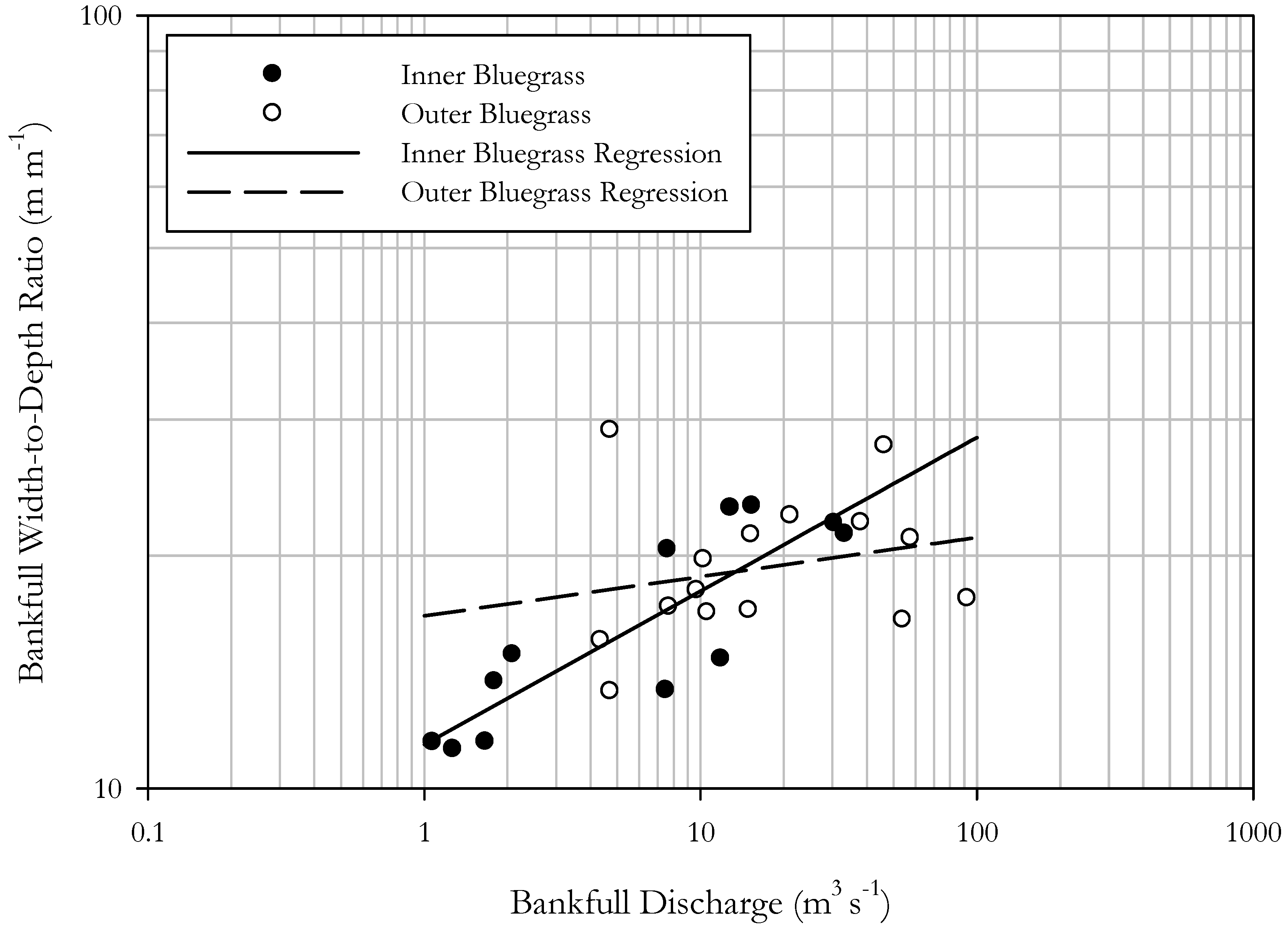
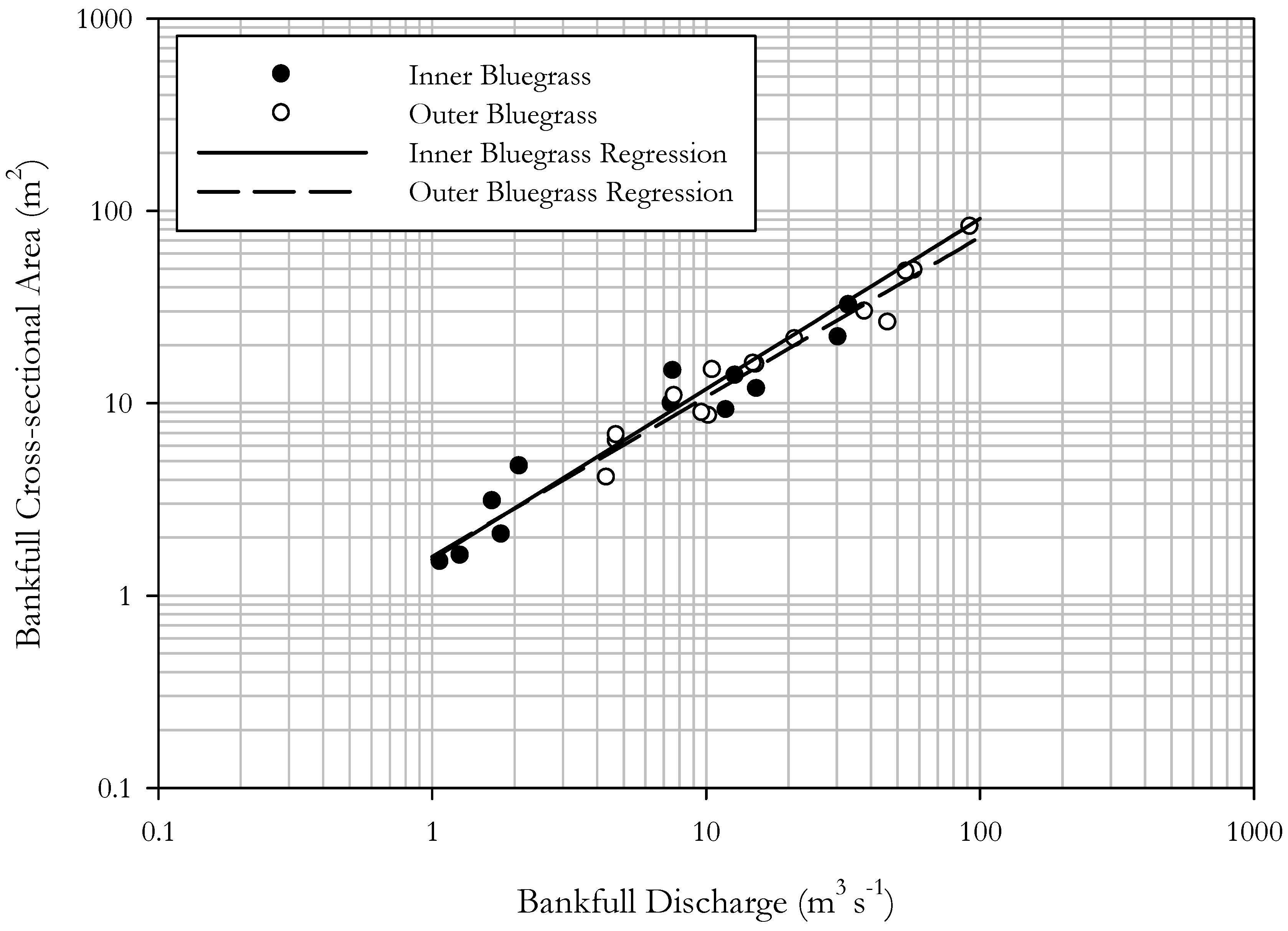
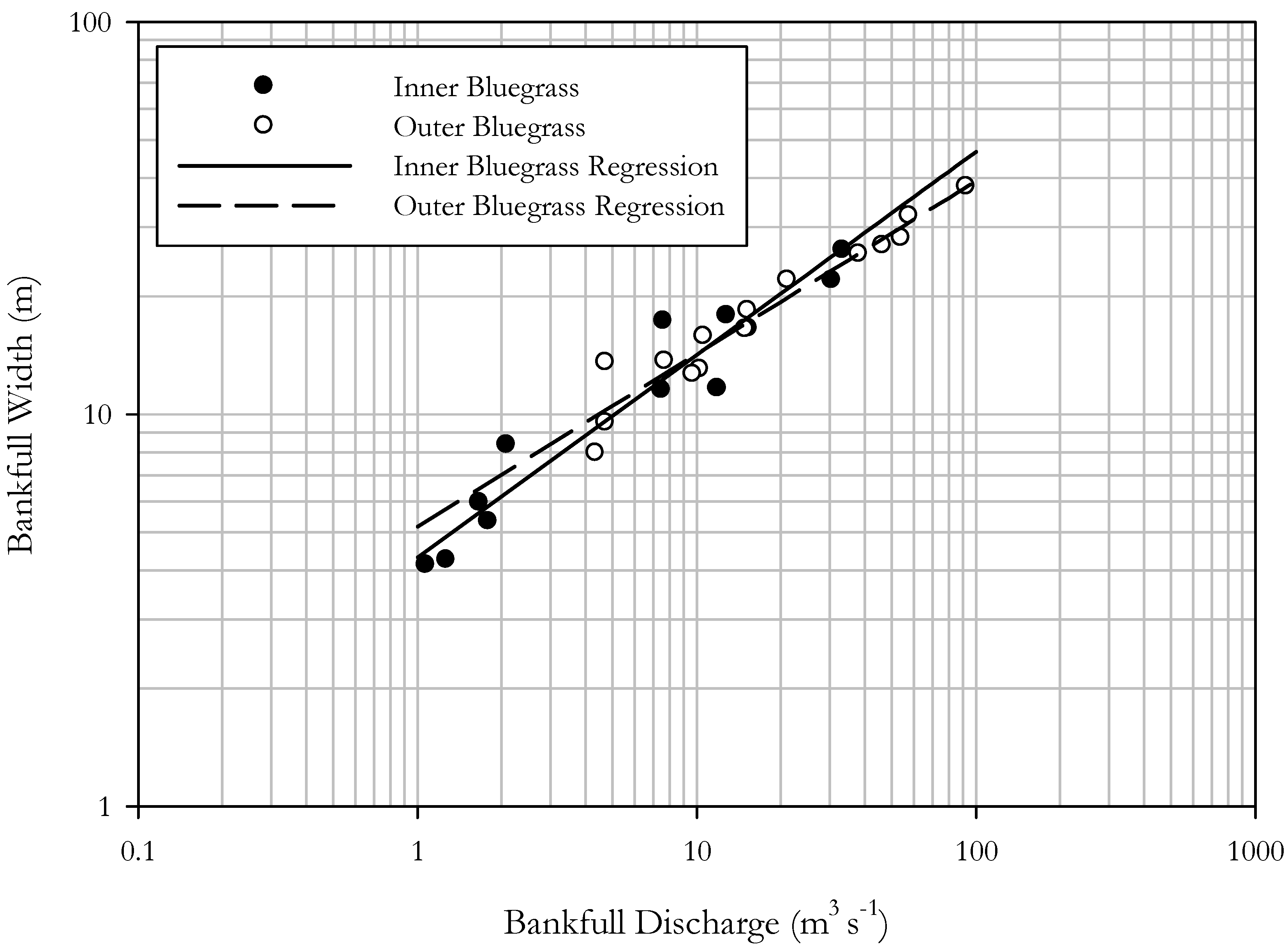
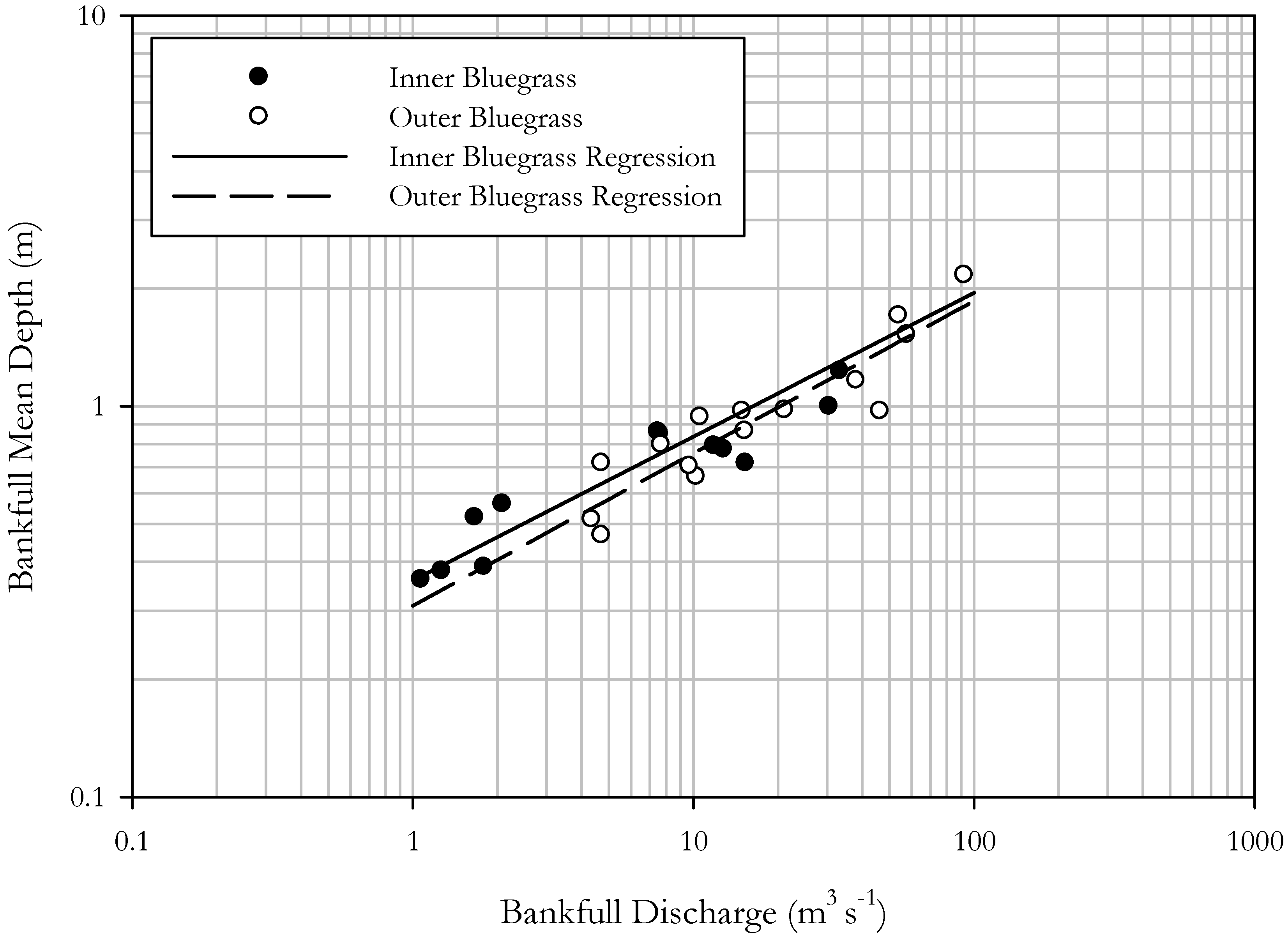
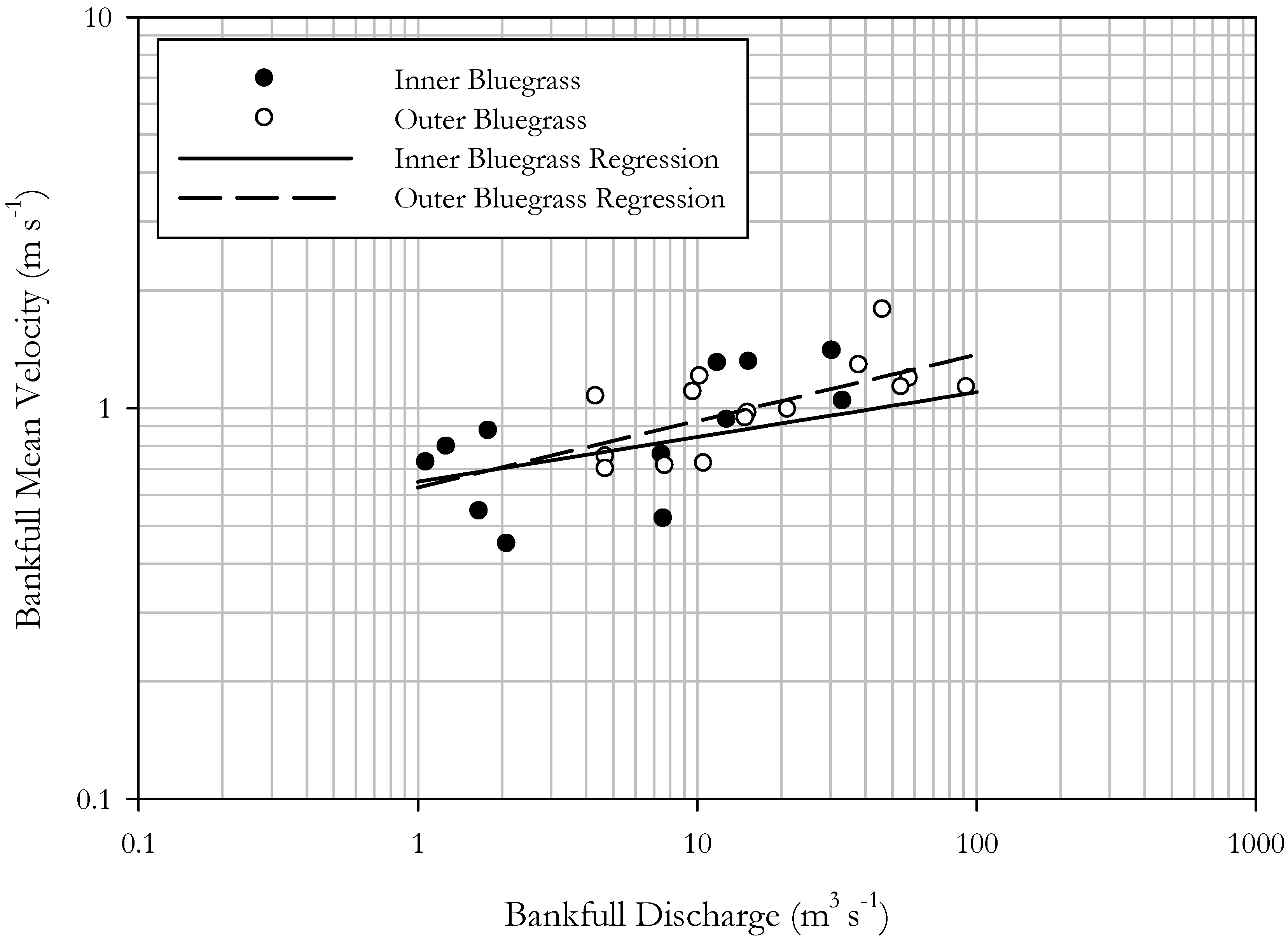
3.1. Bankfull Hydraulic Geometry Curves

Stream morphology data were collected at 12 USGS gaged sites in the Inner Bluegrass for drainage areas between 2.5 and 111 km2 and 15 USGS gaged sites in the Outer Bluegrass for drainage areas between 8.0 and 357 km2 (Table 1). Bankfull discharges ranged from 1.1 to 33.4 m3 s−1 for the
Inner Bluegrass and 4.4 to 92.6 m3 s−1 for the Outer Bluegrass. The percentage of imperviousness was similar between the two regions with values between 0.5 to 29.6 percent measured for the Inner Bluegrass and values between 0.4 to 33.9 percent measured for the Outer Bluegrass (Table 2). For the Inner Bluegrass region, gage sites with higher percentages of imperviousness were not concentrated in smaller watersheds, as might be expected. Rather, higher percentages of imperviousness were measured for gages representing a wide range of watershed sizes. For the Outer Bluegrass region, gages with higher percentages of impervious area tended to be concentrated around Louisville, Kentucky. Land use for the study sites located in the Inner Bluegrass is predominately consists of the categories developed (45.6 ± 21.5 percent) and agriculture (36.7 ± 16.9 percent) with some forest (14.5 ± 13.4 percent) (Table 2). In the Outer Bluegrass, land use is follows a similar pattern with development largest (30.6 ± 25.6 percent); however a greater percentage of land is in forests (35.2 ± 10.5) as compared to agriculture (29.9 ± 16.1 percent).
Table 1. Bankfull summary data for the selected sites in the Inner Bluegrass and Outer Bluegrass regions. Adapted from Brockman et al. [42]. Used by permission from JAWRA.
Site LocationUSGS Gage NumberBankfull Discharge (m3 s-1)Bankfull Cross-Sectional Area (m2)Bankfull Width (m)Bankfull Mean Depth (m)Bankfull Slope (m/m)Bankfull Mean Velocity (m/s)Return Interval (years)Bankfull Indicator1
Inner Bluegrass Region
UT to East Hickman Creek at Chilesburg032845251.31.64.20.40.00630.81.03FDS, ESF
East Hickman Creek at Andover032845201.11.54.10.40.00580.7< 1.01FDS, PBS
Cave Creek near Fort Springs032885001.82.15.30.40.00740.91.27FDS
North Elkhorn Creek at Man O War Rd.032875801.73.15.90.50.00730.51.06FDS, TPB, PBS
North Elkhorn Creek at Winchester Rd.032875902.14.78.40.60.00460.4< 1.01FDS, PBS
Wolf Run at Old Frankfort Pk.0328919311.99.211.60.80.00501.3< 1.01FDS, PBS
East Hickman Creek at Delong Rd.032845307.59.911.50.90.00250.81.01FDS, ESF
West Hickman Creek at Ash Grove Pk.0328455512.913.817.80.80.00340.9< 1.01FDS, ESF
South Elkhorn Creek at Fort Springs0328900015.411.816.50.70.00281.31.17FDS, TPB, PBS
North Elkhorn Creek at Bryan Station Rd.032876007.614.617.30.90.00320.5< 1.01FDS, PBS, ESF
Town Branch at Yarnallton Rd.0328920030.621.921.91.00.00291.41.15FDS, PBS
Eagle Creek at Sadieville0329100033.432.126.21.20.00161.01.24FDS, PBS
Outer Bluegrass Region
Fourmile Creek at Polar Bridge2032387724.44.18.00.50.01841.1< 1.01FDS, PBS, ESF
Chenoweth Run at Ruckriegel Pky.3032981354.76.313.60.50.00530.7< 1.01FDS
Little Goose Creek near Harrods Creek3032924807.710.913.70.80.00610.71.15FDS, ESF
Goose Creek at Old Westport Rd. 3032924744.76.89.50.70.00530.71.09FDS, ESF
Cedar Creek at Hwy 14423032978009.78.912.60.70.00501.11.02FDS, PBS, ESF
North Fork Grassy Creek near Piner20325440010.38.613.00.70.00561.2< 1.01FDS, ESF
Cruises Creek at Hwy 1720325448010.614.815.80.90.00560.7< 1.01FDS, ESF
Middle Fork Beargrass Creek at Old Cannons Ln. 30329300015.016.016.51.00.00370.91.23FDS
Woolper Creek at Woolper Rd. 20326200115.315.818.40.90.00711.0< 1.01FDS, PBS
Banklick Creek at Hwy 182920325455021.221.422.01.00.00511.0< 1.01FDS, ESF
Mud Lick Creek at Hwy 4230327713057.848.732.01.50.00531.2< 1.01FDS, PBS
Gunpowder Creek at Camp Ernst Rd. 20327707546.426.126.91.00.00351.8< 1.01FDS, PBS
Twelvemile Creek at Hwy 199720323874538.229.725.61.20.00251.3< 1.01FDS
Harrods Creek at Hwy 32930329247054.147.928.11.70.00231.11.01FDS, ESF
Floyd’s Fork at Fisherville30329800092.682.138.02.20.00101.1< 1.01FDS, PBS
1 FDS = flat depositional surface immediately adjacent to the stream; TPB = tops of point bars; PBS = prominent breaks in slope; and ESF = erosion or scour features.2 Outer Bluegrass gage sites located near Cincinatti, OH, USA.3 Outer Bluegrass gage sites located near Louisville, KY, USA.
Table 2. Watershed characteristics summary data for the selected sites in the Inner Bluegrass and Outer Bluegrass regions. Adapted from Brockman et al. [42]. Used by permission from JAWRA.
Site LocationUSGS Gage NumberDrainage Area (km2)Percentage Impervious AreaStreamside Vegetation1Land Use (%)
DevelopedForestAgriculture
Inner Bluegrass Region
UT to East Hickman Creek at Chilesburg032845252.53.5Forest42.13.644.2
East Hickman Creek at Andover 032845204.112.0Grass/Forest41.111.346.7
Cave Creek near Fort Springs032885005.021.6Grass64.45.629.7
North Elkhorn Creek at Man O War Rd.032875805.73.2Forest23.717.654.5
North Elkhorn Creek at Winchester Rd.0328759010.59.8Forest31.912.553.2
Wolf Run at Old Frankfort Pk.0328919324.829.6Forest80.614.54.2
East Hickman Creek at Delong Rd.0328453039.113.7Grass44.17.644.1
West Hickman Creek at Ash Grove Pk.0328455553.124.2Forest73.115.19.9
South Elkhorn Creek at Fort Springs0328900054.913.1Forest43.715.539.5
North Elkhorn Creek at Bryan Station Rd.0328760055.712.0Forest33.78.356.6
Town Branch at Yarnallton Rd.0328920077.725.7Grass/Forest62.87.628.5
Eagle Creek at Sadieville03291000111.10.5Forest5.654.529.7
Outer Bluegrass Region
Fourmile Creek at Polar Bridge2032387728.06.5Forest27.939.926.6
Chenoweth Run at Ruckriegel Pky.30329813514.233.9Forest75.715.27.8
Little Goose Creek near Harrods Creek30329248015.018.7Forest64.027.97.1
Goose Creek at Old Westport Rd. 30329247415.511.1Forest51.636.510.3
Cedar Creek at Hwy 144230329780031.30.4Forest5.357.529.2
North Fork Grassy Creek near Piner20325440035.21.0Forest7.740.546.0
Cruises Creek at Hwy 1720325448046.61.2Forest7.239.748.7
Middle Fork Beargrass Creek at Old Cannons Ln. 30329300049.024.4Forest73.720.13.8
Woolper Creek at Woolper Rd. 20326200162.74.1Forest20.938.435.1
Banklick Creek at Hwy 182920325455077.74.5Forest26.633.838.3
Mud Lick Creek at Hwy 4230327713094.33.4Forest15.533.944.6
Gunpowder Creek at Camp Ernst Rd. 20327707594.816.7Forest52.920.721.9
Twelvemile Creek at Hwy 1997203238745101.01.7Forest11.343.038.5
Harrods Creek at Hwy 329303292470182.11.4Forest8.739.948.3
Floyd’s Fork at Fisherville303298000357.42.4Forest13.239.941.9
1 Forest indicates forest dominated; grass indicates grass dominated; forest/grass indicates an approximate equal amount of both.2 Outer Bluegrass gage sites located near Cincinnati, OH, USA.3 Outer Bluegrass gage sites located near Louisville, KY, USA.
Table 3 summarizes hydraulic geometry relationships for the Inner Bluegrass and Outer Bluegrass regions. The exponents for bankfull width, mean depth, and mean velocity followed the order of b > f > m. Pietsch and Nanson [22] and Park [53] noted that this was the typical nonlinear adjustment of a stream to downstream changes in discharge with width being the most sensitive of the three parameters and velocity the least. Fola and Rennie [10] confirmed such a relationship for clay-bed streams suggesting that lateral adjustment is the primary way cohesive-bed channels adjust to increases in discharge. Figure 4, Figure 5, Figure 6, Figure 7, Figure 8 and Figure 9 show the relationship between the bankfull parameters cross-sectional area, width, mean depth, width-to-depth ratio, mean velocity, and slope and bankfull discharge for each region.
The exponents or slopes of the hydraulic geometry equations show strong similarities to other values reported in the literature, as shown in Table 3. For bankfull cross-sectional area, a value of between 0.80 and 0.90 was expected for the exponent based on the theoretical and empirical values presented in the literature [5,23,30,48,54]. For the Inner Bluegrass, the exponent was 0.80; it was 0.83 for the Outer Bluegrass. No statistical difference between the regions was found for bankfull cross-sectional area (p = 0.8626). With regards to bankfull width, an exponent between 0.45 and 0.53 was expected based on theoretical and empirical values [5,23,30,48,54]. Park [53], however, did note that streams in humid temperate regions tended to have width exponents ranging between 0.4 and 0.8. The exponent for the Inner Bluegrass curve of 0.50 was within this range, while the exponent for the Outer Bluegrass was 0.44 was slightly lower than expected but in the range specified by Park [53]. A statistically difference was noted between the curves for the two regions (p = 0.0015). These results indicate that a change in bankfull width for a unit change in bankfull discharge is less for the Outer Bluegrass than for the Inner Bluegrass. As seen in Figure 5, for bankfull discharges less than 10 m3 s−1, streams in the Outer Bluegrass tended to be wider. When bankfull discharges exceeded about 20 m3 s−1, streams in the Inner Bluegrass had a greater tendency to be wider. For bankfull mean depth, theoretical and empirical values indicated that an exponent of about 0.37 should be expected [5,23,30,48,54]. Park [53] found that streams in humid temperate regions tended to have moderate depth exponents generally ranging between 0.2 and 0.6. Both the Inner Bluegrass and Outer Bluegrass had similar values of 0.30 and 0.39, respectively. The Inner Bluegrass exponent was quite similar than the exponent found by Wohl and David [30] for bedrock channels while the Outer Bluegrass exponent was quite similar to that found by Sherwood and Huitger [54] for Ohio streams. While no statistical difference was noted (p = 0.3132), streams in the Inner Bluegrass were slightly deeper than those of the Outer Bluegrass for the same discharge (Figure 6).
Table 3. Hydraulic geometry curves for equations 1, 2, 3, bankfull slope (Sbkf = tQz), and width-to-depth ratio (Wbkf/Dbkf = xQy). Qbkf represents bankfull discharge (m3 s−1), Abkf is bankfull cross-sectional area (m2), Wbkf is bankfull width (m), Dbkf is bankfull mean depth (m), Vbkf is bankfull mean velocity (m s−1), Sbkf is bankfull slope (m m−1), and Wbkf/Dbkf is bankfull width to depth ratio (m m−1).
SourceAbkfWbkfDbkfVbkfSbkfWbkf/Dbkf
ghR2abR2cfR2kmR2tzR2xyR2
Inner Bluegrass1.690.800.934.390.500.930.390.300.870.590.200.420.01−0.320.7211.390.200.73
Outer Bluegrass1.590.830.955.160.440.940.310.390.850.630.170.430.02−0.510.6516.720.050.06
Sherwood and Huitger [54]0.610.870.931.970.500.900.310.370.851.650.130.220.06−0.480.306.400.140.30
Wohl and David [30]-0.803-1.120.500.590.580.300.48---0.08−0.330.281.960.190.09
Leopold et al. [5]1-0.90 --0.53--0.37--0.10--−0.7----
Leopold et al. [5]2-0.903--0.50--0.40--0.10-------
Knighton [23]-0.863-2.610.50-0.310.36--0.14--−0.2----
Hey and Thorne [48]-0.803-3.670.450.790.330.350.80-0.20-------
1Theoretically derived equations for river in downstream direction.2Empirically determined equations for river in downstream direction.3Determined by adding b and f in same row.
Figure 4. Bankfull cross-sectional area vs. bankfull discharge for the Inner Bluegrass and Outer Bluegrass regions.
Water 03 00923 g004
Figure 5. Bankfull width vs. bankfull discharge for the Inner Bluegrass and Outer Bluegrass regions.
Water 03 00923 g005
Figure 6. Bankfull mean depth vs. bankfull discharge for the Inner Bluegrass and Outer Bluegrass regions.
Water 03 00923 g006
Examination of the bankfull width-to-depth ratios versus discharge indicated that the Inner Bluegrass and Outer Bluegrass differed significantly (p = 0.0155). Figure 7 indicates that streams in the Inner Bluegrass tend to be more narrow and deep (i.e., lower width-to-depth ratios) at lower bankfull discharges, and hence smaller drainage areas, than similar streams in the Outer Bluegrass. When bankfull discharges and thus drainage areas increased, streams in the Inner Bluegrass tended to widen slightly faster and become deeper more slowly than those of the Outer Bluegrass. However, as seen in Figure 7, a wide range of scatter is present for the Outer Bluegrass curve as compared to the Inner Bluegrass curve. This scatter is largely driven by three sites in the Louisville, Kentucky area: Chenoweth Run (03298135), Harrods Creek (03292470), and Floyd’s Fork (03298000). Chenoweth Run had the highest width-to-depth ratio of all studied sites while both Harrods Creek and Floyd’s Fork had comparably low width-to-depth ratios for their bankfull discharges. If these three data points were not included, the Inner Bluegrass and Outer Bluegrass curves would not differ (p = 0.1177).
Figure 7. Bankfull width-to-depth ratio vs. bankfull discharge for the Inner Bluegrass and Outer Bluegrass regions.
Water 03 00923 g007
Figure 8. Bankfull mean velocity vs. bankfull discharge for the Inner Bluegrass and Outer Bluegrass regions.
Water 03 00923 g008
Figure 9. Bankfull slope vs. bankfull discharge for the Inner Bluegrass and Outer Bluegrass regions.
Water 03 00923 g009
The reason for the width-to-depth ratio variation at these three sites is not known, but it is hypothesized to be related to physiographic conditions. For example, Chenoweth Run like Goose Creek (03292474) is a highly urbanized watershed. The width of the two streams differs (13.6 m at Chenoweth Run; 9.5 m at Goose Creek). While both streams have similar bankfull discharges (4.7 m3 s−1 at Chenoweth Run; 4.7 m3 s−1 at Goose Creek) and drainage areas (14.2 km2 at Chenoweth Run; 15.5 km2 at Goose Creek), the level of imperviousness is quite different (33.9 percent at Chenoweth Run; 11.1 percent at Goose Creek) (Table 1 and Table 2). Both Cianfrani et al. [55] and Doll et al. [56] found that urbanization increased bankfull channel width as compared to rural streams in the Piedmont region of the U.S. Contrary, Annable et al. [57] found that urbanization did not result in significant channel enlargement for streams in Ontario, Canada. In this study, no trends between percent imperviousness and bankfull width were found for the Outer Bluegrass (Figure 10), so it is likely that the level of urbanization is not the controlling factor for bankfull width. Yet, the question remains as to why the site on Chenoweth Run was wider than expected, and hence produced such a high width to depth ratio. One possibility has to do with riparian vegetation. Hession et al. [49] and Anderson et al. [58] noted that riparian vegetation type exerts an influence on channel width. Hession et al. [49] found that channels with forested riparian buffers were wider than those with grassed riparian buffers. Anderson et al. [58] found that the effect of riparian vegetation type was dependent on watershed size and channel width. For watershed areas greater than 10 km2, as is the case for both Chenoweth Run and Goose Creek, thick forested riparian buffers were associated with narrower channels while grassed and non-forested riparian buffers were associated with wider channels. While both sites had a forested riparian buffer, visual observation indicated that woody vegetation at Goose Creek was much thicker than that at Chenoweth Run. This difference in riparian vegetation thickness may have resulted in a wider channel at Chenoweth Run due in part to differences in rooting depth and density.
Figure 10. Imperviousness vs. bankfull width for the Inner Bluegrass and Outer Bluegrass regions.
Water 03 00923 g010
For Harrods Creek and Floyd’s Fork, it is suspected that the lower than expected width-to-depth ratios, for each stream’s bankfull discharge, are related in part to the geology within the respective watersheds and the streamside riparian vegetation. Adjacent to each other, both watersheds have considerable non-karst formations which differ from the other Outer Bluegrass study sites. As such, bedrock is not exposed along the streambeds at Harrods Creek and Floyd’s Fork. Further, both sites have thick forested riparian vegetation. It is suspected that the lack of a bedrock layer coupled with the thick forested streamside vegetation promoted the development of narrower and deeper channels [58].
With regards to bankfull mean velocity, a value between 0.10 and 0.20 was expected based on the literature [5,23,48,54]. For the Inner Bluegrass, the exponent was 0.20 while it was 0.17 for the Outer Bluegrass. These exponents are higher than that reported by Sherwood and Huitger [54]. No statistical difference was found between the Inner Bluegrass and Outer Bluegrass bankfull velocity curves (p = 0.0596). For bankfull slope, a wide range of values (−0.2 to −0.7) have been reported. Based on work by Sherwood and Huitger [54] for Ohio streams and Wohl and David [30] for bedrock streams, a value between −0.3 and −0.5 was expected. For the Inner Bluegrass, the exponent was -0.32 while it was −0.23 for the Outer Bluegrass. No significant difference were found between the two regions (p = 0.2473).
The R2 values for the bankfull parameters cross-sectional area, width, mean depth, and slope indicate that bankfull discharge explains a large amount of the variability in the morphology of both the Inner Bluegrass and Outer Bluegrass streams. The R2 values for width to depth ratio indicate a good fit for the Inner Bluegrass. However, the R2 values for bankfull mean velocity for the Inner Bluegrass and Outer Bluegrass as well as width-to-depth ratio for only the Outer Bluegrass indicated a poorer fit. While the values of the exponents of the bankfull mean velocity hydraulic geometry equations were similar to those found by in the literature [5,23,48,54], the low R2 values were due to scatter in the data. Channel characteristics such as roughness factors associated with bed material, bedforms, vegetation, and slope influence mean velocity [46]. It is likely that combinations of these factors are the cause of the scatter associated with bankfull mean velocity. As for width-to-depth ratios for the Outer Bluegrass, local geologic variations, coupled with riparian vegetation thickness, is suspected to be the reason for the scatter in these data.
Based on the continuity equation, multiplying the coefficients for bankfull width, mean depth, and mean velocity resulted in a value of 1.0 for both the Inner Bluegrass and Outer Bluegrass. Summing the exponents for these same parameters also resulted in a value of 1.0 for both regions. These results agree with work by Leopold and Maddock [4] in their development of hydraulic geometry theory.

3.2. Bankfull Return Intervals

Bankfull return intervals ranged from < 1.01 to 1.27 years for the Inner Bluegrass region and from < 1.01 to 1.23 years for the Outer Bluegrass. These return intervals are less than the average value of 1.5 years presented by Leopold et al. [5]. Powell et al. [14] found that the bankfull return interval ranged from 0.6 to 1.4 years for large rivers (drainage area of 75 km2 or greater) in Ohio. Metcalf et al. [44] also found bankfull return intervals in these ranges for the northern regions of Florida. Such return intervals also agree with values found by stream restoration practitioners working in the Inner Bluegrass and Outer Bluegrass [59].

4. Conclusions

Twenty-seven USGS gaged stream reaches were surveyed to determine their bankfull dimensions, discharges, and return intervals for this study. These data were used to develop bankfull hydraulic geometry relationships for the Inner Bluegrass and Outer Bluegrass regions of Kentucky. Exponents of the developed curves agree well with theoretical and empirically-derived values in the literature [5,23,30,48,54]. With the exception of bankfull width and width-to-depth ratio, the Inner Bluegrass and Outer Bluegrass hydraulic geometry curves were statistically similar. While Johnson and Fecko [34] found that a single equation could be used to scale bankfull width for the Valley Ridge, Appalachian Plateau, and New England physiographic regions, such was not the case with the Inner Bluegrass and Outer Bluegrass regions. Inner Bluegrass streams tended to be more narrow and deep for bankfull discharges less than 10 m3 s-1 and wider and shallower for bankfull discharges greater than 20 m3 s−1. Three sites within the Outer Bluegrass strongly influenced the width and width-to-depth relationships. Removing these three sites produced an Outer Bluegrass curve (revised coefficient x = 11.23; revised exponent y = 0.20) that was equivalent to the Inner Bluegrass curve. However, removing these points did not result in the same width relationship between the Outer Bluegrass (revised coefficient a = 4.43; revised exponent b = 0.49) and Inner Bluegrass regions (p = 0.0015). Based on the strong similarities in coefficient and exponent values for the width hydraulic geometry relationships between the two regions when the three sites were removed, this lack of difference is thought to be a false.
Development and comparison of hydraulic geometry relationships for the Inner and Outer Bluegrass regions highlighted the importance of local-scale geology and riparian vegetation on the channel dimensions bankfull width and depth, even for relatively small physiographic regions. For the Inner Bluegrass where geologic variations were small, width-to-depth ratio showed little variation in scaling with discharge. However, for the Louisville area of the Outer Bluegrass region where the geology is more variable, the scatter was greater in the width-to-depth relationship. Based on the influence of geology, even within a physiographic region, it is recommended that additional research be conducted to develop hydraulic geometry relationships for other physiographic regions, particularly in karst-influenced areas.
Practitioners involved in stream assessment and restoration are guided to separate hydraulic geometry relationships on a physiographic region basis. However, this study suggests that in some instances, evaluation is needed on a watershed basis within a physiographic region while in others, curves across hydrophysiographic regions may not differ. Understanding the extent to which hydraulic geometry relationships are applicable is warranted, particularly in karst settings.
It has been postulated that streams in karst-influenced areas would have smaller discharges, and hence smaller channel dimensions, than streams in non-karst areas with the same drainage areas due to a suspected greater extent of discharge conveyance via subsurface conduits [39]. The results of this study suggest that this may not necessarily be the case for the Inner Bluegrass and Outer Bluegrass regions. For example, hydraulic geometry curves for the karst-influenced Inner and Outer Bluegrass regions (average of 14.1 and 8.8 percent imperviousness, respectively) have similar exponents and coefficients to those presented Harman et al. [60] for the rural streams in the Piedmont of North Carolina, an area that does not have karst features [61]. For a 25 km2 drainage area, the Inner Bluegrass relationships predict values of bankfull discharge, cross-sectional area, width and mean depth of 7.1 m3 s−1, 8.3 m2, 11.6 m, and 0.7 m, respectively. For the Outer Bluegrass, these values are 9.1 m3 s−1, 9.7 m2, 13.5 m, and 0.8 m, respectively. For the North Carolina Piedmont, these values are 13.0 m3 s−1, 9.2 m2, 9.8 m, and 0.9 m, respectively. On the other hand, the scaling relationships developed by Wohl and David [30] for bedrock channels world-wide would predict a much greater bankfull discharge (62.4 m3 s-1), smaller width (8.5 m), and greater depth (1.9 m) than the Inner Bluegrass and Outer Bluegrass relationships. These differences may be related to climatic and riparian vegetation influences. Both the Piedmont of North Carolina and the Bluegrass Region of Kentucky have similar climates and vegetation types whereas many of the sites studied by Wohl and David differ markedly (e.g., western U.S.). As such, the karst-influenced streams in this study may scale in a similar manner to other streams in differing physiographic regions, but similar climatic patterns, despite the degree of karst-influence. Additional research on the potential influence of varying extents of karst on hydraulic geometry relations is warranted.

Acknowledgements

This study was funded by a 319(h) grant from the U.S. Environmental Protection Agency (Award Number: P02-590-0700010583) and the University of Kentucky College of Agriculture through the Senate Bill 271 program. The investigation reported in this paper is part of a project of the Kentucky Agricultural Experiment Station and is published with approval of the Director. Mention of trade names or commercial products does not constitute endorsement or recommendation for use. The authors would like to thank Teri Dowdy for her assistance with Arc GIS and Joshua Howard and Kyle Brockman for their assistance with the field work. The authors would also like to thank the three anonymous reviewers for providing insightful comments.

References and Notes

  1. Dunne, T.; Leopold, L.B. Water in Environmental Planning; W.H. Freeman: New York, NY, USA, 1978. [Google Scholar]
  2. Shields, F.D.; Copeland, R.R.; Klingeman, P.C.; Doyle, M. W.; Simon, A. Design for stream restoration. J. Hydraul. Eng. 2003, 129, 575–584. [Google Scholar] [CrossRef]
  3. Singh, V.P. On the theories of hydraulic geometry. Int. J. Sediment Transport 2003, 18, 196–218. [Google Scholar]
  4. Leopold, L.B.; Maddock, T. The Hydraulic Geometry of Stream Channels and Some Physiographic Limitations; U.S. Geological Survey Professional Paper 252; United States Government Printing Office: Washington, DC, USA, 1953. [Google Scholar]
  5. Leopold, L.B.; Wolman, M.G.; Miller, J.P. Fluvial Processes in Geomorphology; Dover Publications: New York, NY, USA, 1964. [Google Scholar]
  6. Copeland, R.R.; Biedenharn, D.S.; Fischenich, J.C. Channel Forming Discharge; ERDC/CHL CHETN-VIII-5; U.S. Army Corps of Engineers: Washington, DC, USA, 2000. [Google Scholar]
  7. Williams, G.P. Bankfull discharge of rivers. Water Resour. Res. 1978, 14, 1141–1154. [Google Scholar] [CrossRef]
  8. Andrews, E.D. Effective and bankfull discharge of streams in the Yampa River Basin, Colorado and Wyoming. J. Hydrol. 1980, 46, 311–330. [Google Scholar] [CrossRef]
  9. Radecki-Pawlik, A. Bankfull discharge in mountain streams: Theory and practice. Earth Surf. Processes and Landforms 2002, 27, 115–123. [Google Scholar] [CrossRef]
  10. Fola, M.E.; Rennie, C.D. Downstream hydraulic geometry of clay-dominated cohesive bed rivers. J. Hydraul. Eng. 2010, 136, 524–527. [Google Scholar] [CrossRef]
  11. Wolman, M.G.; Miller, J.P. Magnitude and frequency of geomorphic processes. J. Geol. 1960, 68, 54–74. [Google Scholar] [CrossRef]
  12. Wolman, M.G. A Cycle of sedimentation and erosion in urban river channels. Geografiska Annaler 1967, 49A, 385–395. [Google Scholar] [CrossRef]
  13. Emmett, W.W.; Wolman, M.G. Effective discharge and gravel-bed rivers. Earth Surf. Processes and Landforms 2001, 26, 1369–1380. [Google Scholar] [CrossRef]
  14. Powell, G.E.; Mecklenberg, D.; Ward, A. Evaluating channel-forming discharges: A study of large rivers in Ohio. Trans ASABE 2006, 49, 35–46. [Google Scholar] [CrossRef]
  15. Afzalimehr, H.; Abdolhosseini, M.; Singh, V.P. Hydraulic geometry relations for stable channel design. J. Hydraul. Eng. 2010, 15, 859–864. [Google Scholar] [CrossRef]
  16. Andrews, E.D.; Nankervis, J.M. Effective discharge and the design of channel maintenance flows for gravel-bed rivers. In Natural and Anthropogenic Influences in Fluvial Geomorphology; Costa, J.E., Miller, A.J., Potter, K.W., Wilcock, P.R., Eds.; American Geophysical Union: Washington, DC, USA, 1995; Geophysical Monograph 89; pp. 151–164. [Google Scholar]
  17. Annable, W.K.; Lounder, V.G.; Watson, C.C. Estimating channel-forming discharge in urban watercourses. River Res. Appl. 2011, 27, 738–753. [Google Scholar] [CrossRef]
  18. Stall, J.B.; Yang, C.T. Hydraulic Geometry of 12 Selected Streams of the United States; Research Report No. 32; University of Illinois Water Resources Center: Urbana-Champaign, IL, USA, 1970. [Google Scholar]
  19. Lane, E.W. The importance of fluvial morphology in hydraulic engineering. Proc. Am. Soc. Civ. Eng. 1955, 81, 1–17. [Google Scholar]
  20. Davis, W.M. Studies for students: Base-level, grade, and peneplain. J. Geol. 1902, 10, 77–111. [Google Scholar] [CrossRef]
  21. Wolman, M.G. The Natural Channel of Brandywine Creek, Pennsylvania; U.S. Geological Survey Professional Paper 282; United States Government Printing Office: Washington, DC, USA, 1955.
  22. Pietsch, T.J.; Nanson, G.C. Bankfull hydraulic geometry; the role of in-channel vegetation and downstream declining discharges in the anabranching and distributary channels of the Gwydir distributive fluvial system, Southeastern Australia. Geomorphology 2011, 129, 152–165. [Google Scholar] [CrossRef]
  23. Knighton, A.D. Fluvial Forms and Processes; Edward Arnold: London, England, UK, 1998. [Google Scholar]
  24. Knighton, A.D. Short-term changes in hydraulic geometry. In River Channel Changes; Gregory, K.J., Ed.; John Wiley & Sons: New York, NY, USA, 1977. [Google Scholar]
  25. Castro, J.M.; Jackson, P.L. Bankfull discharge recurrence intervals and regional hydraulic geometry relationships: Patterns in the Pacific Northwest, USA. JAWRA 2001, 37, 1249–1262. [Google Scholar]
  26. Emmett, W.W. The Channels and Waters of the Upper Salmon River, Idaho; U.S. Geological Survey Professional Paper 870A; United States Government Printing Office: Washington, DC, USA, 1975.
  27. Dury, G.H. Discharge prediction, present and former, from channel dimensions. J. Hydrol. 1976, 30, 219–245. [Google Scholar] [CrossRef]
  28. Julien, P.Y.; Wargadalam, J. Alluvial channel geometry: Theory and applications. J. Hydraul. Eng. 2006, 121, 312–325. [Google Scholar] [CrossRef]
  29. Lee, A.M.; Julien, P.Y. Downstream hydraulic geometry of alluvial channels. J. Hydraul. Eng. 2006, 132, 1347–1352. [Google Scholar] [CrossRef]
  30. Wohl, E.; David, G.C.L. Consistency of scaling relations among bedrock and alluvial channels. J. Geophys. Res. 2008. [Google Scholar] [CrossRef]
  31. Montgomery, D.R.; Gran, K.B. Downstream variations in the width of bedrock channels. Water Resour. Res. 2001, 37, 1841–1846. [Google Scholar] [CrossRef]
  32. Sudduth, E.B.; Meyer, J.L.; Bernhardt, E.S. Stream restoration practices in the Southeastern United States. Restoration Ecol. 2007, 15, 573–583. [Google Scholar] [CrossRef]
  33. Natural Resources Conservation Service. Stream Restoration Design Handbook. National Engineering Handbook Part 654 (NED-654); United States Department of Agriculture: Washington, DC, USA, 2007.
  34. Johnson, P.A.; Fecko, B.J. Regional channel geometry equations: A statistical comparison for physiographic provinces in the Eastern US. River Res. Appl. 2008, 24, 823–834. [Google Scholar] [CrossRef]
  35. Keaton, J.N.; Messinger, T.; Doheny, E.J. Development and Analysis of Regional Curves for Streams in the Non-Urban Valley and Ridge Physiographic Province, Maryland, Virginia, and West Virginia; Scientific Investigations Report 2005-0576; U.S. Geological Survey: Reston, VA, USA, 2005.
  36. Currens, J.C. Kentucky is Karst Country! What You Should Know about Sinkholes and Springs; Information Circular 4; Series XII; Kentucky Geological Survey: Lexington, KY, USA, 2002. [Google Scholar]
  37. The Bluegrass Region; Kentucky Geological Survey: Lexington, KY, USA, 2007. Available online: http://www.uky.edu/KGS/geoky/regionbluegrass.htm (accessed on 30 October 2010).
  38. McDowell, R.C. The Geology of Kentucky—A Text to Accompany the Geologic Map of Kentucky; Professional Paper 1151-H; U.S. Geologic Survey: Washington, DC, USA, 1986. [Google Scholar]
  39. Parola, A.C.; Vesely, W.S.; Croasdaile, M.A.; Hansen, C.; Jones, M.S. Geomorphic Characteristics of Streams in the Bluegrass Physiographic Region of Kentucky; Kentucky Division of Water: Frankfort, Kentucky, USA, 2007. [Google Scholar]
  40. Peake, T.; Schumann, R.R. Regional Radon Characterizations. In Field Studies of Radon in Rocks, Soil and Water; Gunderson, L.C.S., Wanty, R.B., Eds.; C.K. Smoley: Boca Raton, FL, USA, 1993. [Google Scholar]
  41. National Climatic Data Center. Climatography of the United States No. 81. Monthly Station Normals of Temperature, Precipitation, and Heating and Cooling Degree Days 1971-2000: 15 Kentucky; National Oceanic and Atmospheric Administration: Asheville, NC, USA, 2002. [Google Scholar]
  42. Brockman, R.R.; Agouridis, C.T.; Workman, S.R.; Ormsbee, L.E.; Fogle, A.R. Bankfull regional curves for the Inner and Outer Bluegrass regions of Kentucky. JAWRA. (Submitted).
  43. Leopold, L.B. A View of the River; Harvard University Press: Cambridge, MA, USA, 1994. [Google Scholar]
  44. Metcalf, C.K.; Wilkerson, S.D.; Harman, W.A. Bankfull regional curves for North and Northwest Florida streams. JAWRA 2009, 45, 1260–1272. [Google Scholar]
  45. Harrelson, C.C.; Rawlins, C.; Potyondy, J. Stream Channel Reference Sites: An Illustrated Guide to Field Techniques; USDA Forst Service Rocky Mountain Forest and Range Experiment Station General Technical Report RM245; United States Printing Office: Washington, DC, USA, 1994. [Google Scholar]
  46. McCuen, R.H. Hydrologic Analysis and Design; Prentice-Hall: Upper Saddle River, NJ, USA, 2004. [Google Scholar]
  47. Ward, A.; D’Ambrosio, J.L.; Witter, J. Channel-Forming Discharges, Fact Sheet AEX-445-03; The Ohio State University Extension: Columbus, OH, USA, 2008. [Google Scholar]
  48. Hey, R.D.; Thorne, C.R. Stable channels with mobile gravel beds. J. Hydraul. Eng. 1986, 112, 671–689. [Google Scholar] [CrossRef]
  49. Hession, W.C.; Pizzuto, J.E.; Johnson, T.E.; Horwitz, R.J. Influence of bank vegetation on channel morphology in rural and urban watersheds. Geology 2003, 31, 147–150. [Google Scholar] [CrossRef]
  50. United States Geological Survey. Bulletin 17B, Guidelines for Determining Flood-Flow Frequency; Hydrology Subcommittee of the Interagency Advisory Committee on Water Data: Reston, VA, USA, 1982. [Google Scholar]
  51. Hodgkins, G.A.; Martin, G.R. Estimating the Magnitude of Peak Flows for Streams in Kentucky for Selected Recurrence Intervals; Water Resources Investigations Report 03-4180; United States Government Printing Office: Washington, DC, USA, 2003. [Google Scholar]
  52. SAS. SAS User’s Guide Version 9; SAS Institute: Cary, NC, USA, 2008. [Google Scholar]
  53. Park, C.C. World-wide variations in hydraulic geometry exponents of stream channels: An analysis and some observations. J. Hydrol. 1977, 33, 133–146. [Google Scholar] [CrossRef]
  54. Sherwood, J.M.; Huitger, C.A. Bankfull Characteristics of Ohio Streams and Their Relation to Peak Streamflows; Scientific Investigations Report 2005-5153; U.S. Geological Survey: Reston, VA, USA, 2005.
  55. Cianfrani, C.M.; Hession, W.C.; Rizzo, D.M. Watershed imperviousness impacts on stream channel condition in Southeastern Pennsylvania. JAWRA 2006, 42, 941–956. [Google Scholar]
  56. Doll, B.A.; Wise-Frederick, D.E.; Buckner, C.M.; Wilderson, S.D.; Harman, W.A.; Smith, R.E.; Spooner, J. Hydraulic geometry relationships for urban streams throughout the Piedmont of North Carolina. JAWRA 2002, 38, 641–651. [Google Scholar]
  57. Annable, W.K.; Watson, C.C.; Thompson, P.J. Quasi-equilibrium conditions of urban gravel-bed stream channels in Southern Ontario, Canada. River Res. Appl. 2010. [Google Scholar] [CrossRef]
  58. Anderson, R.J.; Bledsoe, B.P.; Hession, W.C. Width of streams and rivers in response to vegetation, bank material, and other factors. JAWRA 2004, 40, 1159–1172. [Google Scholar]
  59. Athanasakes, G.; Stantec Consulting, Louisville, KY, USA. Personal communication, 2010.
  60. Harman, W.A.; Jennings, G.D.; Patterson, J.M.; Clinton, D.R.; Slate, L.O.; Jessup, A.G.; Everhart, J.R.; Smith, R.E. Bankfull hydraulic geometry relationships for North Carolina streams. In AWRA Summer Symposium; Olsen, D.S., Potyondy, J.P., Eds.; Wildland Hydrology: Bozeman, MT, USA, 1999. [Google Scholar]
  61. Veni, G. Revising the karst map of the United States. J. Cave Karst Stud. 2002, 64, 45–50. [Google Scholar]

