Application of Copula Functions for Rainfall Interception Modelling


Faculty of Civil and Geodetic Engineering, University of Ljubljana, 1000 Ljubljana, Slovenia
*
Author to whom correspondence should be addressed.
Water 2018, 10(8), 995; https://doi.org/10.3390/w10080995
Submission received: 20 June 2018
/
Revised: 25 July 2018
/
Accepted: 26 July 2018
/
Published: 27 July 2018
(This article belongs to the Special Issue Advances in Multivariate Analysis of Environmental Phenomena: Celebrating the 15th Anniversary of Copulas in Hydrology)
Abstract
:Rainfall interception is an important process of the water cycle that can have significant influence on surface runoff and groundwater storage. Since rainfall interception measurements are rare and time consuming, rainfall interception estimation can be made indirectly using different meteorological variables. Experimental data of rainfall interception for birch and pine trees was measured at an experimental plot located in an urban area of Ljubljana, Slovenia in this study. A copula model was applied to predict the rainfall interception using meteorological variables, namely air temperature and vapour pressure deficit data. The copula model performance was compared to some other models such as decision trees, multiple linear regressions, and exponential functions. Using random sampling, we found that the copula model where Khoudraji-Liebscher copula functions were used yielded slightly smaller root mean square error (RMSE) and mean absolute error (MAE) values than other tested methods (i.e., RMSE and MAE results for birch trees were 24.2% and 18.2%, respectively and RMSE and MAE results for pine trees were 25.0% and 19.6%, respectively). The results demonstrate that the copula-based proposed method and other tested models could be used for the prediction of rainfall interception at the considered plot and in the wider surroundings. Furthermore, these models could also be applied for the prediction of rainfall interception for these two tree species in other locations under similar vegetation and meteorological conditions.
1. Introduction
Rainfall interception by vegetation is recognized as an important process of the hydrological cycle by researchers worldwide, influencing surface runoff in a great manner, irrespective of whether they are conducted in natural or urban forests (e.g., [1,2,3,4,5,6]). Rainfall partitioning can be divided into three main components, namely throughfall, stemflow, and interception loss. Throughfall is a portion of precipitation that either reaches the ground directly without touching the canopy or reaches the ground at a later time by dripping from the saturated canopy. Stemflow is a portion of intercepted precipitation that reaches the ground by flowing down the branches and stem. Interception loss is a portion of rainfall that is intercepted by the vegetation and evaporated back into the atmosphere, never reaching the ground. The process of rainfall partitioning is influenced by different meteorological (e.g., rainfall amount, intensity, raindrop size, raindrop velocity, air temperature, air humidity, wind speed) and vegetation variables (e.g., tree type, canopy characteristics, stem roughness, leaf area index) [4,7,8,9,10,11,12,13,14]. Rainfall amount, duration and intensity are often recognised as the most influential meteorological variables since they decrease rainfall interception [4,14,15,16,17]. However, throughfall and stemflow, both of which also decrease rainfall interception, continue after the end of the rainfall event [13,18]. In this extended period, the evapotranspiration, highly influenced by air humidity and air temperature, plays a significant role in the rainfall partitioning process [4,15,19].
Rainfall interception measurements are quite complicated and time consuming as they take years of fieldwork [14,20,21]. However, meteorological variables such as air temperature and relative air humidity measurements that are needed to calculate the vapour pressure deficit are usually available from national meteorological stations, or they can be measured using fairly simple and cheap equipment. Thus, from a practical point of view, a model that can be used to predict rainfall interception loss for specific vegetation and climatic conditions using only climatic data is needed. However, at least some experimental measurements are needed to construct the model. More specifically, all vegetation periods (e.g., at least one leafed and one leafless period) should be recorded in order to detect the seasonal variability in rainfall interception. Different statistical methods (e.g., [9,12,17,22]) and other model types (e.g., [4,23,24,25,26]) have already been used and developed to evaluate the influence of different variables on rainfall interception, and also to predict it. Some models are quite complex, requiring a large number of parameters. For example, the Gash interception model [27] requires parameters such as canopy cover fraction, canopy storage capacity, rainfall necessary to saturate the canopy and others (e.g., [4,25,27]). Moreover, as input parameters, throughfall and stemflow data need to be considered (e.g., [4,25,27]). Furthermore, the Gash model [27] was developed based on the Rutter model [28] and requires less data than the initial model version [25]. Similarly, the two-layer stochastic model requires estimation of several parameters and consideration of additional input variables [23,24]. To simplify rainfall interception evaluation and modelling, we decided to try copula models, which were not yet applied to the rainfall partitioning data.
De Michele and Salvadori [29] were the first to introduce copula functions for applications in hydrology. Since then, the number of papers that apply copula functions to different hydrological problems has increased. For example, a Web of Science database search using the “copula” topic in the Water Resources category indicates that in 2016 and 2017, more than 70 papers per year were published including this keyword, while in 2010, only 29 papers were published. Salvadori and De Michele were first to carry out multivariate frequency analysis via copula functions [30] and different multivariate design strategies were first discussed by Salvadori et al. [31]. Moreover, copula functions have been used several times for rainfall analysis and modelling. Some examples of this include: for rainfall frequency analysis in order to estimate reliable design rainfall (e.g., [32,33,34,35,36,37]), for disaggregation of rainfall data (e.g., [38,39]), to construct intensity-duration-frequency (IDF) curves for different purposes (e.g., [40,41,42]), for rainfall generation and modelling (e.g., [43,44,45]), for drought analyses and characterisation of drought properties (e.g., [46,47,48,49,50,51,52,53,54,55,56,57]), and for other rainfall related analyses (e.g., [58,59,60,61,62,63,64]). However, one should bear in mind that research dealing with copula functions is also very intense in the Statistics Probability category (e.g., more than 250 papers were published in 2017 in this category according to the Web of Science database). This means that the topic is also relevant from the statistical and mathematical perspective, and that consequently, with the development of the research area, we can expect even more applications of copulas in the future.
The main aim of this study was to compare the performance of the copula model for the estimation of the rainfall interception loss using air temperature (T) and vapour pressure deficit (VPD) data with some other estimation techniques, namely exponential function, multiple linear regression, and decision trees. The idea was not to use rainfall measurements in the model construction, but rather other meteorological variables because in some cases, rainfall data is not available and relative humidity and air temperature can also be measured using easily available digital sensors, which means that fieldwork is not needed. The performance of the above-mentioned models is evaluated using 175 rainfall events from an experimental plot in Slovenia where birch and pine trees are present. The specific aims of the study are as follows: (i) to fit the copula and some other models to the data; (ii) to compare the performance of tested methods and (iii) to compare the evaluation results with respect to two different tree species (birch and pine tree).
2. Materials and Methods
2.1. Rainfall Partitioning Measurements
Rainfall in the open, throughfall and stemflow were measured in a park in the city of Ljubljana, Slovenia (46.04° N, 14.49° E) [13,14,65]. The typical climate for the area is temperate continental with well-defined seasons. The mean long-term (1986–2016) total annual rainfall is approximately 1380 mm and the average annual temperature is 11 °C, which varies between ‒3 °C in the winter and 24 °C in the summer [66]. The study plot has an area of approximately 600 m2 and is covered with grass (Figure 1). In the western part of the plot, a group of birch trees (Betula pendula Roth) and a group of pine trees (Pinus nigra Arnold) grow. There is no overlapping between the two groups of trees. Measurements of interception by two different tree species in our study were conducted in an urban area. Therefore, the basic research on rainfall interception was focused on the benefits of urban trees as part of green infrastructure [14,67]. One of the benefits of such urban trees is the storm water reduction [67]. Although trees have an important role in regulating urbanised hydrology systems, there is still little known about the best trees to choose. Since, in addition to meteorological variables, vegetation variables also have a large influence on the interception, each new research on additional tree species is an important contribution to the field.
The height of birch trees is on average 15.7 m (±1.0 m) with a total projected crown area of 42.3 m2 and an average diameter at breast height of 17.9 cm. The pine trees are on average 12.6 m (±0.6 m) high, have a total projected crown area of 22.7 m2 and an average diameter at breast height of 19.0 cm (±2.3 cm). The birch tree canopy is characterized by upwards branch inclination (51° on average from the stem to the branch) and a leaf area index (LAI) of 0.8 in leafless and 2.3 in the leafed period (measured with a LAI-2200 plant canopy analyser). The pine tree branches are inclined downwards (on average 98° from the stem to the branch) and the LAI values are on average equal to 3.8 (±0.7). Birch trees have smoother bark with a storage capacity of 0.7 mm, while the bark of pine trees is rougher and more absorptive, with a 3.5 mm bark storage capacity [14].
The measurements were conducted from 1 January 2014 to 30 June 2017. The rainfall in the open was measured with a tipping bucket (0.2 mm/tip) rain gauge (Onset RG2-M) with an automatic data logger (Onset HOBO Event). The equipment was located in the clearing at the study plot, 10 m from the nearest tree. In the observed period, a total of 413 rainfall events were detected. After further analysis, 175 rainfall events were taken into account, as snow events and events with incomplete data were excluded.
Throughfall was measured with through- and funnel-type gauges in order to consider throughfall spatial variability (Figure 1). Under each group of trees, two through gauges (catch area of 7.5 m2) were positioned from the tree stem towards the edge of the canopy. One was connected to a tipping bucket flow gauge (Unidata 6506G; 50 mL/tip) and an automatic data logger (Onset HOBO Event), while the other was connected to a manually-read polyethylene barrel (60 L capacity), collected after each event. Under each group of trees, ten manually-read funnel-type gauges (catch area of 78.5 cm2) were also randomly placed and moved around during the three and half years of measurements [65].
Stemflow was measured for one representative tree in each group. Around the stem, a halved rubber hose was spirally wrapped, capturing the water flowing down the stem. In the case of pine trees, it was collected in manually-read 1.5 L container, while in the case of birch trees, the rubber hose was connected to a tipping bucket (Onset RG2-M, 0.2 mm/tip) with an automatic data logger (Onset HOBO Event). The contribution area of the tree canopy was used to convert stemflow volume to its depth [17,68,69].
2.2. Meteorological Variables
According to the rainfall and throughfall measurements with an automatic data logger at the study plot, rainfall amount, duration, and intensity were determined for each rainfall event. Events were separated by at least a 4 h dry period. Based on the defined beginning and end of the rainfall event, the minimum air temperature (TMIN), maximum air temperature (TMAX), average air temperature (T) and average relative humidity (RH) per event were also calculated. We have used the half-hour data (air temperature and relative humidity) measured at the location of the Ljubljana-Bežigrad meteorological station in the Ljubljana city area [66], located 3 km from the study plot. According to the Slovenian Environment Agency, its measurements are representative for the whole city and its neighborhood due to its special location in the Ljubljana basin [70]. The FAO Penman-Monteith methodology was applied for the vapour pressure deficit (VPD) calculations [71]. The following equations were used to derive the vapour pressure deficit (VPD), calculated as es-ea (es is saturation vapour pressure and ea is actual vapour pressure) using the minimum air temperature (TMIN), maximum air temperature (TMAX) and average relative humidity (RH) data derived using half-hourly data from the beginning to the end of each rainfall event:
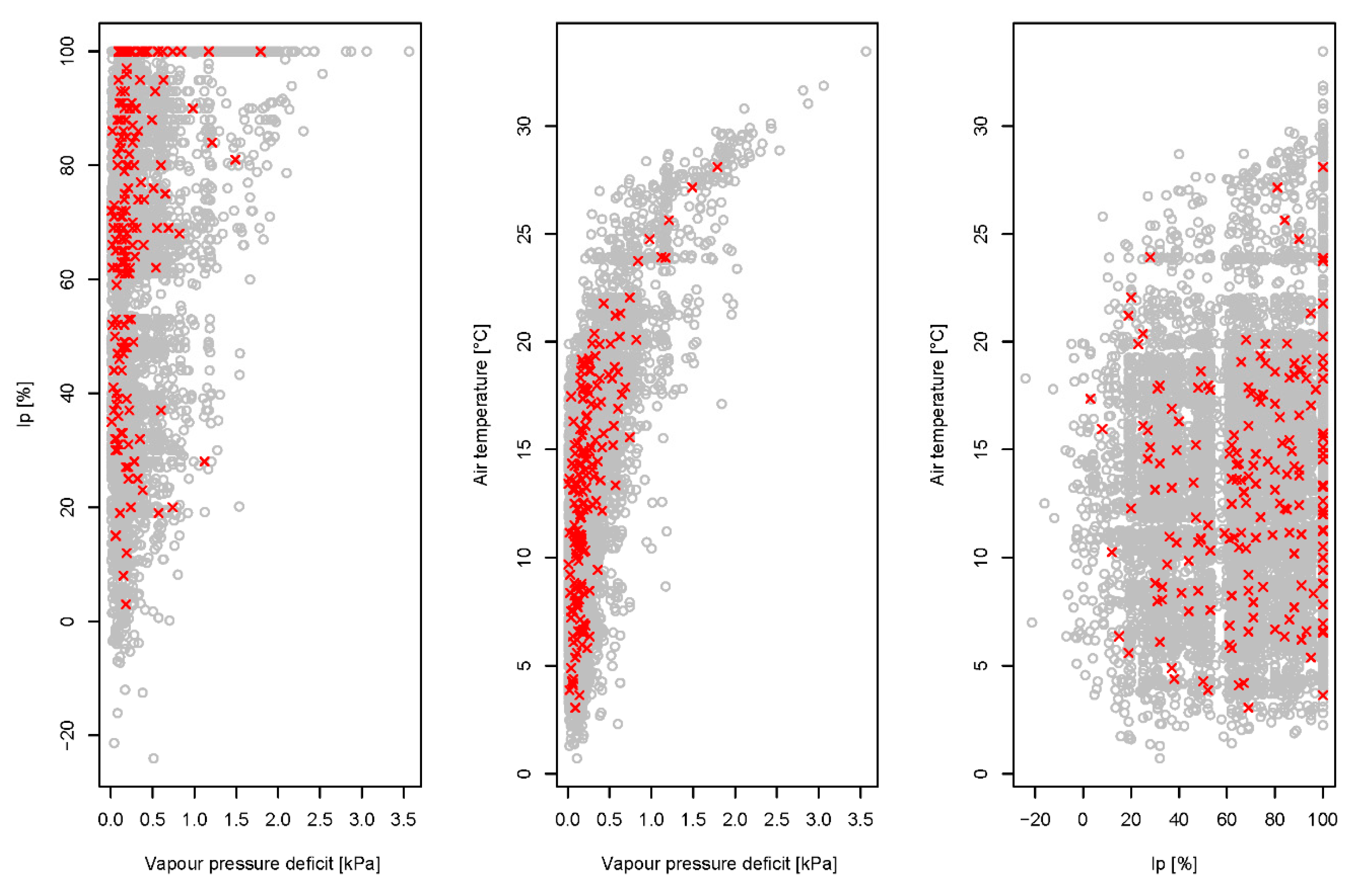
Figure 2 shows the relationship between air temperature, vapour pressure deficit and interception loss for birch (Ib) and pine (Ip) trees for the 175 events that were analysed in this study. Events measured in the leafless and leafed period are indicated with red and black colour, respectively. About 20% of all considered events were measured in the leafless period, and 80% in the leafed period. The correlation between Ib and T, and Ip and T, is similar for the leafless and leafed periods. On the other hand, the correlation between Ib and VPD, and Ip and VPD, is higher for events measured in the leafless period than for events measured in the leafed period (Figure 2). Furthermore, correlation between T and VPD was higher during the events that were measured in the leafed period compared to the events measured in the leafless period (Figure 2).
2.3. Copulas
Before fitting the copula model, the independence of consecutive events was examined. The Ljung-Box test was used for this purpose, whereas the Box.test function that is implemented in the R software was used [72]. Copulas are functions that connect joint multivariate probability distributions with univariate marginal distribution functions [73]. A detailed description of copula functions in general and their main characteristics is available in [74,75,76,77]. The definition of the Khoudraji-Liebscher copula functions applied in this study can be found in [78,79]. These copulas were first introduced and discussed in hydrology by [80,81], and are applied in this study based on the conclusions made by Bezak et al. [82], who have applied Khoudraji-Liebscher copula functions for the estimation of suspended sediment loads. The symmetric Archimedean copulas C1 and C2 were used (Equation (6)) for the estimation of the interception loss based on the vapour pressure deficit (VPD) and air temperature (T) data for the birch and pine trees, respectively. The suitability of this copula function was tested using the procedure described below, and several tests results are presented in Section 3.2. For the three-dimensional case study that was analysed here, the cumulative distribution function is as follows [78,79]:
where α1, α2, α3 are shape parameters, are the two copula functions, are the parameters of these two copula functions (u1 = FVPD(VPD), u2 = FI(I) and u3 = FT(T)).
The parameters of the copula functions were estimated using the maximum pseudo-likelihood method [83,84]. As are symmetric, Joe, Frank, Clayton and Gumbel-Hougaard copula functions were used (Table 1). Thus, in total, 16 different combinations of Khoudraji-Liebscher copulas were tested. More information about the selected Archimedean copula functions can be found in [76]. The exchangeability was tested using the exchTest function that is part of the R software copula package (symmetric copulas can be used when variables are exchangeable) [72,84]. Moreover, the Cramér-von Mises test Sn was applied to test the adequacy of different copula models [85]. Furthermore, the xvCopula function implemented in the R software copula package was used to select the most suitable copula for the estimation of the interception loss [84,86]. The k-fold cross-validation was applied to estimate the xvCopula results, which means that samples were divided into k equal sized samples. k-1 sub-samples were used as training data and one sub-sample was used for validation. This procedure was repeated k times to obtain model selection criterion results (each of the k sub-samples was used once for validation). In order to deal with ties in the data, the so-called “first” method was applied in the process of data ordering (i.e., this method uses a permutation with increasing values at each index set of ties [72]). The non-parametric distribution function defined by Hutson [87] and Serinaldi [88] was applied as a marginal distribution function. The term “copula model” is used for the combination of the non-parametric distributions and Khoudraji-Liebscher copulas in the next part of the paper.
2.4. Other Models Used for Estimation of Rainfall Interception and Performance Criteria
The copula model described in Section 2.3 was compared to several other models. Similarly to Bezak et al. [82], we also tested the exponential model (EXP) with two parameters (only the vapour pressure deficit variable was used as input in this model) and the multiple regression model (MLR) (VPD and T were used) considering three parameters. The parameters were estimated using the least-square method. The EXP method was selected due to its simplicity compared to other tested methods. The R software usdm package and vifstep function were used to test for multicollinearity [72,89]. Additionally, we also tested the decision tree model. Decision trees are one of the data mining techniques that can be used to construct a model for the prediction of target variables based on selected influential variables. We used continuous numeric values of interception loss as the target variable and air temperature and vapour pressure deficit as influential variables. Constructed decision trees are composed from nodes and leaves [90]. Additional information about tree structure is defined within tree nodes (i.e., usually the mean and variance of instances related to one specific node and values that are used to divide different nodes). Moreover, each leaf is associated with the predicted value of the target variable. The tree depth was limited to five levels and we did not split subsets smaller than five. The final number of nodes and leaves was not the same for the two tree species (birch and pine), and the fitted models are presented in Section 3. Using these regression models and information about nodes, one can calculate rainfall interception based on VPD and T variables. The Orange software [91] was applied for the construction of the decision tree.
For the evaluation of the tested models (copula, exponential, multiple linear regression and decision tree), random sampling was used. The training set size was 75% and test set size was 25%. The random sampling procedure was repeated 20 times (n = 20). Root mean square error (RMSE) and mean absolute error (MAE) criteria were used to compare the model results. Additionally, to check the sensitivity of the RMSE and MAE results regarding the training and test set size, we also repeated the previously described procedure using 50% of events for training and 50% for validation. For the copula model, 10,000 possible Ib and Ip values were generated based on known pairs of variables T and VPD (for the test set). Similarly to Bezak et al. [82], we used the median value of 10,000 realizations as the estimated rainfall interception value for birch and pine trees.
3. Results and Discussion
3.1. Rainfall Interception and Influencing Variables
From three and a half years of measurements, we selected 175 rainfall events with complete data for further analysis. The total rainfall amount for these events was 2049 mm and average intensity was 2.0 mm/h (±2.4 mm/h). The largest event in terms of rainfall amount was detected between 14 and 15 June 2016, with a total rainfall amount of 93 mm and a duration of 21.5 h. Table 2 shows the descriptive statistics for the analyzed variables used in this study. On average, birch trees intercepted 40% (±27%) of rainfall per event (Table 2). The interception loss was equal to 100% for 12 events with less than 1.4 mm of rainfall in the open (Figure 3). This was expected, since for the events with a rainfall amount smaller than the canopy storage capacity (1.1–3.5 mm for birch trees), the total rainfall amount is intercepted [14]. Furthermore, for three events, throughfall under birch trees exceeded the amount of rainfall in the open, which resulted in negative values of rainfall interception (Table 2). This phenomenon is usually attributed to so called “drip points”, where rain drops concentrate at the edge of the canopy e.g., [4,65]. Pine trees intercepted on average 68% (±25%) of rainfall per event (Table 2). The entire rainfall amount in the open was intercepted during 29 events with less than 2.6 mm of rainfall (canopy storage capacity for pine trees varied between 0.9 and 2.9 mm) (Figure 3). In total, birch trees intercepted 484.8 mm of rainfall (24%) and pine trees intercepted 926.5 mm of rainfall (45%). Compared to similar deciduous trees, the rainfall interception of birch trees was in the range of 20% and 29% of rainfall measured in oak and birch deciduous forest in the UK [92], 25% and 28% measured in mixed Mediterranean deciduous forest in Slovenia [4] and between 16% and 25% measured in a temperate deciduous forest in Maryland, USA [93]. Interception losses by pine trees in the present study are similar to 41% of gross precipitation measured in mature coniferous forest in British Columbia, Canada [94], 52% rainfall intercepted by Douglas-fir and 61% intercepted by western red cedar in an urban area of North Vancouver, Canada [95].
3.2. Selection of the Most Suitable Copula Function
The main idea of the copula application was to estimate the rainfall interception loss using only meteorological variables, namely T and VPD data. Before fitting any model to the data autocorrelation, the marginal data was tested. Ljung-Box test results were 3.8 (p-value 0.07), 0.001 (p-value: 0.99), 2.1 (p-value: 0.15) and 0.25 (p-value: 0.62) for Ib, Ip, T and VPD, respectively. This means that there was no significant autocorrelation in the data, which indicates that data transformation is not needed. Table 3 shows the calculated Kendall’s correlation coefficients values for the following pairs of variables: I-T, I-VPD and T-VPD for birch and pine trees, respectively. Using the Fisher r-to-z transformation, we also tested the significance of the difference between two correlation coefficients for birch and pine trees. The calculated test statistics and p-values were −0.75 (p-value 0.45), 1.08 (p-value 0.28) and 0.11 (p-value 0.90) for I-T, I-VPD and T-VPD, respectively. This means that the calculated correlation coefficients were not significantly different for all three pairs of variables with the selected significance level of 0.05. In the process of the copula model construction, we focused on the Khoudraji-Liebscher copula functions where we used symmetric Archimedean copulas C1 and C2 from Equation (6) [78,79,80,81,82]. Moreover, exchangeability test results for birch trees were 0.09 (p-value 0.05), 0.07 (p-value 0.85) and 0.03 (p-value 0.98) for Ib-T, Ib-VPD and T-VPD, respectively. On the other hand, the exchangeability results for pine trees were 0.12 (p-value 0.84), 0.19 (p-value 0.77) and 0.03 (p-value 0.98) for Ip-T, Ip-VPD and T-VPD, respectively. This means that variables are exchangeable and the copulas shown in Table 1 can be used as C1 and C2 functions.
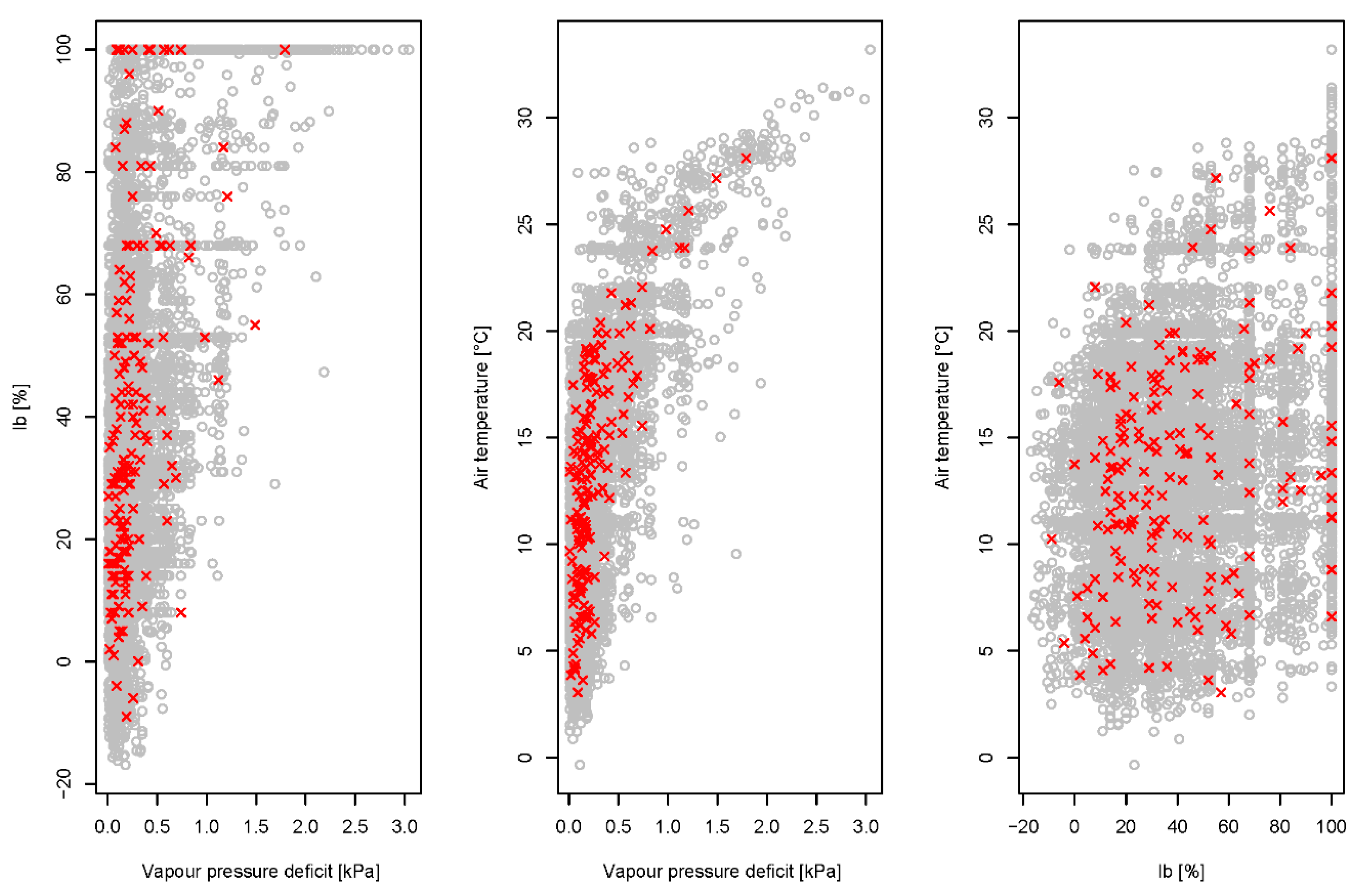
Different combinations of Khoudraji-Liebscher copulas were tested where Joe, Clayton, Gumbel-Hougaard and Frank copulas were applied as C1 and C2 (Section 2.3). Thus, in total, 16 combinations were tested for both trees using the Cramér-von Mises test. For birch trees, the following combinations of C1-C2 could not be rejected with the selected significance level of 0.05: Gumbel-Hougaard-Joe, Gumbel-Hougaard-Gumbel-Hougaard, Joe-Gumbel-Hougaard, Joe-Joe, Frank-Gumbel-Hougaard, Clayton-Gumbel-Hougaard and Clayton-Joe. For all these combinations, the model selection criteria that is based on k-fold cross-validation was used (Section 2.3), and the following results (i.e., the cross-validated log likelihood defined by [84,86]) were 50.88, 52.95, 60.62, 51.17, 45.27, 59.54 and 37.81 for the Gumbel-Hougaard-Joe, Gumbel-Hougaard-Gumbel-Hougaard, Joe-Gumbel-Hougaard, Joe-Joe, Frank-Gumbel-Hougaard, Clayton-Gumbel-Hougaard and Clayton-Joe combinations, respectively. Based on the presented results, the Joe-Gumbel-Hougaard copula was selected as the most suitable for the birch tree data (the maximum model selection criterion result was obtained for this combination). For this copula function, the estimated copula parameters () were 2.59 and 1.74, and the shape parameters (α1, α2, α3) were 0.24, 0.92 and 0.07. For the complete copula model (non-parametric distribution function and Joe-Gumbel-Hougaard copulas as C1 and C2), we also visually checked the fit between the measured data and data generated using the previously mentioned model (Figure 4).
A similar procedure was also carried out for the pine tree data. Using the Cramér-von Mises test, the following combinations of Archimedean copulas as C1 and C2 could not be rejected with the selected significance level of 0.05: Gumbel-Hougaard-Joe, Gumbel-Hougaard-Gumbel-Hougaard, Joe-Gumbel-Hougaard, Joe-Joe, Frank-Joe, Clayton-Gumbel-Hougaard and Clayton-Joe. Furthermore, the most suitable copula was selected using the model selection criteria presented in Section 2.3. The calculated results (i.e., the cross-validated log likelihood defined by [84,86]) were 17.29, 17.84, 31.55, 21.81, 13.35, 30.61 and 21.04 for the Gumbel-Hougaard-Joe, Gumbel-Hougaard-Gumbel-Hougaard, Joe-Gumbel-Hougaard, Joe-Joe, Frank-Joe, Clayton-Gumbel-Hougaard and Clayton-Joe combinations, respectively. Similarly, as for the birch trees, the same combination of Archimedean copula functions were used as C1 and C2 (Joe-Gumbel-Hougaard was used because the maximum model selection criterion result was obtained for this combination). The estimated copula parameters for were 2.73 and 1.86, respectively. Furthermore, the estimated shape parameters were 0.21, 0.99 and 0.06 for the α1, α2 and α3, respectively. Figure 5 shows the graphical comparison between generated data for pine trees using the fitted copula model and measured data.
3.3. Comparison of Copula Results with Other Models
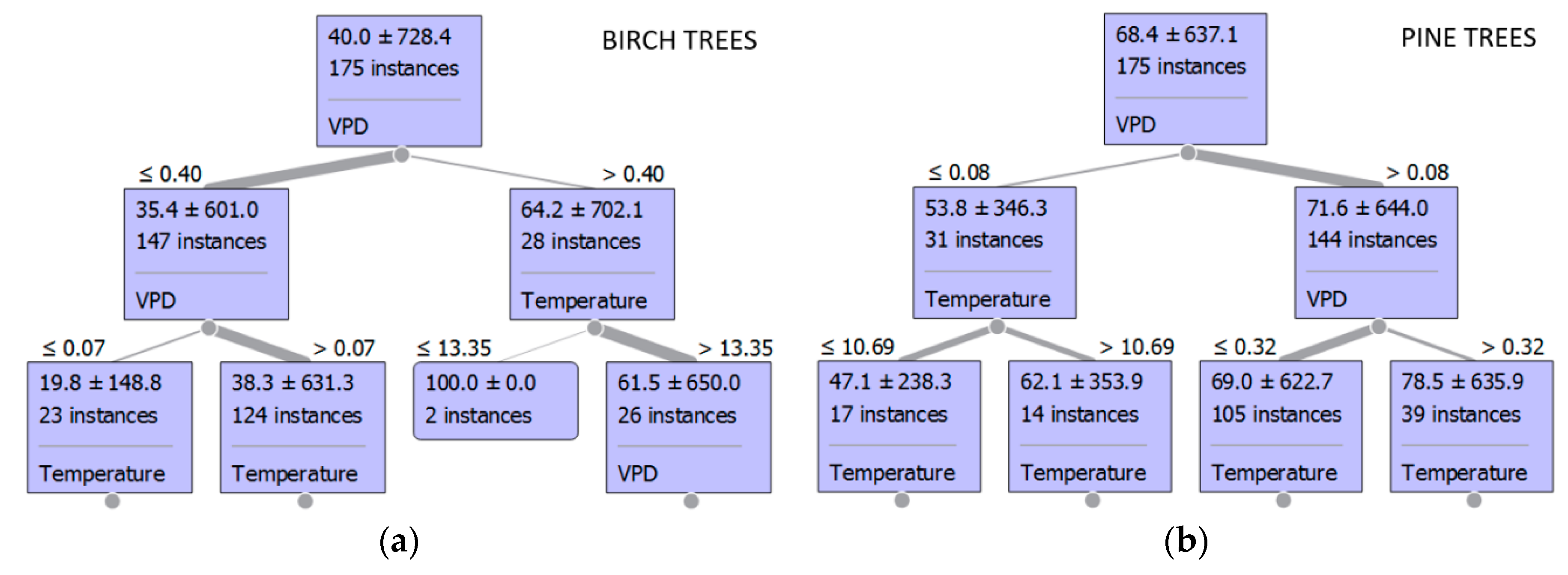
In the next step of the study, we compared copula model performance with some other methods that are described in Section 2.4. Firstly, the parameters of the EXP and MLR methods were estimated. The EXP and MLR models of rainfall interception for birch trees (Ib) were Ib = exp(4.2) × VPD0.32 and Ib = 31.34 + VPD × 41.62 − T × 0.15, respectively. Moreover, the EXP and MLR models of rainfall interception for pine trees (Ip) were Ip = exp(4.39) × VPD0.10 and Ip = 67.47 + VPD × 24.92 − T × 0.41, respectively. The variance inflation factor (VIF) and the test for multicollinearity (implemented in the usdm package [89] that is part of the R software [72]) were used to check if there is any collinearity issues in the data. The results indicate that no input variable has a collinearity problem (VIF values were 1.05, 1.94 and 2.0 for Ip, T and VPD, respectively; VIF values were 1.17, 1.93 and 2.12 for Ib, T and VPD, respectively). A VIF value larger than 10 would indicate that a model has a collinearity issue [72,89]. In the next step, a decision tree was fitted to the data. In total (at all five levels), 25 nodes and 13 leaves were determined for birch trees and 27 nodes and 14 leaves were determined for pine trees (Figure 6). According to the decision trees, the most influential variable on rainfall interception by both considered tree species was VPD as it was the top split variable in both cases (Figure 6). However, the splitting values differ significantly for pine and birch trees. More specifically, much lower splitting values of VPD were determined in the case of pine trees (0.08 kPa) than in the case of birch trees (0.40 kPa). These values were determined in the process of decision tree calibration and can be seen in Figure 6. Additionally, rainfall interception is, on average, lower with lower VPD values for both tree species.
According to all models, higher VPD values in general increase rainfall interception regardless of the tree species. This finding is in accordance with Staelens et al. [9], who demonstrated that vapour pressure deficit significantly increased rainfall interception by a single beech throughout the year. However, in the case of stemflow, a high negative correlation with VPD was observed for yellow poplar and American beech [12]. According to the results of the MLR model, increasing air temperature decreased rainfall interception, whereas the results of the decision trees showed a different response of rainfall interception to changes in air temperature according to the VPD values. According to the decision trees, the rainfall interception for both considered tree species was negatively correlated with temperature for VPD higher than 0.32 kPa and 0.40 kPa for pine and birch trees, respectively. Previous analysis with the regression trees also showed that the interception by pine trees decreased with an increase in the temperature [14]. However, larger stemflow amounts and negative rainfall interception at low temperatures were observed for a single beech [9], while warm wind and increasing air temperature in a Mediterranean deciduous forest decreased throughfall and therefore increased rainfall interception [4]. Some differences in the observed rainfall interception in response to the air temperature may be also the consequence of a different number of the variables considered in the studies.
Table 4 shows results of the RMSE and MAE model evaluation criteria that were used to compare the tested models. The results indicate relatively similar behaviour of the tested models, where the differences among models are relatively small compared to the accuracy of the models. However, a slightly better performance according to the RMSE and MAE criteria was observed for the copula model. Better results could be obtained with the inclusion of additional variables in the models. However, additional variables would also increase the number of parameters used (e.g., one additional variable would increase the number of parameters for the MLR method from three to four, and for the copula method from five to six). The number of parameters for the decision tree is mainly constrained by the selected minimum tree depth and other parameters. On the other hand, in the exponential model, it is not possible to include additional variables. Furthermore, the exponential function also yielded similar results than the other tested models despite its simplicity (two parameters, one input variable). Interestingly, for the decision tree model, RMSE and MAE results were slightly higher than for the copula model despite a larger number of parameters being involved. Moreover, besides firstly applied random sampling (the training set size 75% and test set size 25%), which was used in the study, we also calculated RMSE and MAE results using 50% of events for calibration and 50% for validation. The calculated results were slightly worse than using procedure shown in Table 4. However, the maximum differences were up to 6% (i.e., 6% higher RMSE and MAE values were obtained). Moreover, we were also not able to detect any significant differences among the tested methods. This could indicate that the results presented in Table 4 are not sensitive to the relationship between the size of the training and test sets.
4. Conclusions
The presented paper shows the results of rainfall interception modelling using only meteorological variables usually available from national meteorological stations, namely air temperature and vapour pressure deficit data. The interception loss is an important process of the hydrological cycle and has an important influence on the surface runoff and groundwater storage, among others. Since rainfall interception measurements are complicated and very time consuming, a methodology that can be used to model rainfall interception for specific vegetation and climatic conditions using only climatic data is needed. However, at least some experimental measurements are needed to calibrate the model. More specifically, all vegetation periods (e.g., at least one leafed and one leafless period) should be recorded in order to detect the seasonal variability in rainfall interception. Based on the presented results, the following conclusions can be made:
- The Khoudraji-Liebscher copula model, which has previously been used in a relatively similar application by Bezak et al. [82], can be successfully applied for the estimation of rainfall interception based on air temperature and vapour pressure deficit data.
- The performance of the copula model is relatively similar to the performance of other tested methods. However, according to the RMSE and MAE criteria, slightly better results are obtained using copula functions compared to the other tested methods in this study. The performance of the models could be further improved with the inclusion of other additional variables in the models; however, this would generally increase the complexity of the models. For the EXP method, additional variables cannot be added. For the MLR and copula models, one additional variable would mean one additional parameter. For the decision tree method, the number of parameters is not only connected with the number of variables used, but also with other settings such as maximal tree depth.
- The copula method yielded similar performance for both birch and pine trees despite the fact that the correlation (Table 3) between I-T and I-VPD was smaller for pine trees compared to birch trees. However, correlations between I-T and I-VPD for birch and pine trees were not significantly different with a significance level of 0.05. The constructed models could also be applied for the prediction of rainfall interception under similar vegetation and meteorological conditions in other locations where these two tree species are present. In the case of a longer data series, a different model could be constructed for the leafless and leafed periods.
Author Contributions
M.Š., N.B. and K.Z. drafted the manuscript and determined the aims of the research; K.Z. collected and analysed the rainfall interception data; N.B. developed the models used; All authors contributed to the interpretation of the results, manuscript writing and revision.
Acknowledgments
The results of the study are part of the research Programme P2-0180: “Water Science and Technology, and Geotechnical Engineering: Tools and Methods for Process Analyses and Simulations, and Development of Technologies” that is financed by the Slovenian Research Agency (ARRS). We wish to thank the Slovenian Environment Agency (ARSO) for making data publically available.
Conflicts of Interest
The authors declare no conflict of interest.
References
- Waterloo, M.J.; Bruijnzeel, L.A.; Vugts, H.F.; Rawaqa, T.T. Evaporation from Pinus caribaea plantations on former grassland soils under maritime tropical conditions. Water Resour. Res. 1999, 35, 2133–2144. [Google Scholar] [CrossRef]
- Putuhena, W.M.; Cordery, I. Some hydrological effects of changing forest cover from eucalypts to Pinus radiata. Agric. For. Meteorol. 2000, 100, 59–72. [Google Scholar] [CrossRef]
- Grace, J.M.; Skaggs, R.W.; Chescheir, G.M. Hydrologic and water quality effects of thinning Loblolly Pine. Am. Soc. Agric. Biol. Eng. 2006, 49, 645–654. [Google Scholar]
- Šraj, M.; Brilly, M.; Mikoš, M. Rainfall interception by two deciduous Mediterranean forests of contrasting stature in Slovenia. Agric. For. Meteorol. 2008, 148, 121–134. [Google Scholar] [CrossRef] [Green Version]
- Armson, D.; Stringer, P.; Ennos, A.R. The effect of street trees and amenity grass on urban surface water runoff in Manchester, UK. Urban For. Urban Green. 2013, 12, 282–286. [Google Scholar] [CrossRef]
- Inkiläinen, N.M.; McHale, M.R.; Blank, G.B.; James, A.L.; Nikinmaa, E. The role of the residential urban forest in regulating throughfall: A case study in Raleigh, North Carolina, USA. Landsc. Urban Plan. 2013, 119, 91–103. [Google Scholar] [CrossRef]
- Crockford, R.H.; Richardson, D.P. Partitioning of rainfall into throughfall, stemfow and interception: Effect of forest type, ground cover and climate. Hydrol. Process. 2000, 14, 2903–2920. [Google Scholar] [CrossRef]
- Nanko, K.; Hotta, N.; Suzuki, M. Evaluating the influence of canopy species and meteorological factors on throughfall drop size distribution. J. Hydrol. 2006, 329, 422–431. [Google Scholar] [CrossRef]
- Staelens, J.; De Schrijver, A.; Verheyen, K.; Verhoest, N.E.C. Rainfall partitioning into throughfall, stemflow, and interception within a single beech (Fagus sylvatica L.) canopy: Influence of foliation, rain event characteristics, and meteorology. Hydrol. Process. 2008, 22, 33–45. [Google Scholar] [CrossRef]
- Van Stan, J.T.; Siegert, C.M.; Levia, D.F.; Scheick, C.E. Effects of wind-driven rainfall on interception and stemflow generation between two codominant tree species with differing crown characteristics. Agric. For. Meteorol. 2011, 151, 1277–1286. [Google Scholar] [CrossRef]
- Zabret, K. The influence of tree characteristics on rainfall interception. Acta Hydrotech. 2013, 26, 99–116. (In Slovenian) [Google Scholar]
- Van Stan, J.T.; Van Stan, J.H.; Levia, D.F. Meteorological influences on stemflow generation across diameter size classes of two morphologically distinct deciduous species. Int. J. Biometeorol. 2014, 58, 2059–2069. [Google Scholar] [CrossRef] [PubMed]
- Zabret, K.; Rakovec, J.; Mikoš, M.; Šraj, M. Influence of Raindrop Size Distribution on Throughfall Dynamics under Pine and Birch Trees at the Rainfall Event Level. Atmosphere 2017, 8, 240. [Google Scholar] [CrossRef]
- Zabret, K.; Rakovec, J.; Šraj, M. Influence of meteorological variables on rainfall partitioning for deciduous and coniferous tree species in urban area. J. Hydrol. 2018, 558, 29–41. [Google Scholar] [CrossRef]
- Xiao, Q.; McPherson, E.G.; Ustin, S.L.; Grismer, M.E.; Simpson, J.R. Winter rainfall interception by two mature open-grown trees in Davis, California. Hydrol. Process. 2000, 14, 763–784. [Google Scholar] [CrossRef]
- Toba, T.; Ohta, T. An observational study of the factors that influence interception loss in boreal and temperate forests. J. Hydrol. 2005, 313, 208–220. [Google Scholar] [CrossRef]
- Siegert, C.M.; Levia, D.F. Seasonal and meteorological effects on differential stemflow funneling ratios for two deciduous tree species. J. Hydrol. 2014, 519, 446–454. [Google Scholar] [CrossRef]
- Iida, S.; Levia, D.F.; Shimizu, A.; Shimizu, T.; Tamai, K.; Nobuhiro, T.; Kabeya, N.; Noguchi, S.; Sawano, S.; Araki, M. Intrastorm scale rainfall interception dynamics in a mature coniferous forest stand. J. Hydrol. 2017, 548, 770–783. [Google Scholar] [CrossRef]
- Guevara-Escobar, A.; Gonzalez-Sosa, E.; Veliz-Chavez, C.; Ventura-Ramos, E.; Ramos-Salinas, M. Rainfall interception and distribution patterns of gross precipitation around an isolated Ficus benjamina tree in an urban area. J. Hydrol. 2007, 333, 532–541. [Google Scholar] [CrossRef]
- Muzylo, A.; Llorens, P.; Domingo, F. Rainfall partitioning in a deciduous forest plot in leafed and leafless periods. Ecohydrology 2012, 5, 759–767. [Google Scholar] [CrossRef]
- Van Stan, J.T.; Coenders-Gerrits, M.; Dibble, M.; Bogeholz, P.; Norman, Z. Effects of phenology and meteorological disturbance on litter rainfall interception for a Pinus elliottii stand in the southeastern United States. Hydrol. Process. 2017, 31, 3719–3728. [Google Scholar] [CrossRef]
- Nanko, K.; Hudson, S.A.; Levia, D.F. Differences in throughfall drop size distributions in the presence and absence of foliage. Hydrol. Sci. J. 2016, 61, 620–627. [Google Scholar] [CrossRef]
- Calder, I.R. Dependence of rainfall interception on drop size: 1. Development of the two-layer stochastic model. J. Hydrol. 1996, 185, 363–378. [Google Scholar] [CrossRef]
- Hall, R.L. Interception loss as a function of rainfall and forest types: Stochastic modelling for tropical canopies revisited. J. Hydrol. 2003, 280, 1–12. [Google Scholar] [CrossRef]
- Su, L.; Zhao, C.; Xu, W.; Xie, Z. Modelling interception loss using the revised Gash model: A case study in a mixed evergreen and deciduous broadleaved forest in China. Ecohydrology 2016, 9, 1580–1589. [Google Scholar] [CrossRef]
- Huang, J.Y.; Black, T.A.; Jassal, R.A.; Les Lavkulich, L.M. Modelling rainfall interception by urban trees. Can. Water Resour. J. 2017, 42, 336–348. [Google Scholar] [CrossRef]
- Gash, J.H.C.; Lloyd, C.R.; Lachaud, G. Estimating sparse forest rainfall interception with an analytical model. J. Hydrol. 1995, 170, 79–86. [Google Scholar] [CrossRef]
- Rutter, A.J.; Kershaw, K.A.; Robins, P.C.; Morton, A.J. A predictive model of rainfall interception in forests, I. Derivation of the model from observations in a stand of Corsican pine. Agric. Meteorol. 1971, 9, 367–384. [Google Scholar] [CrossRef]
- De Michele, C.; Salvadori, G.A. Generalized Pareto intensity-duration model of storm rainfall exploiting 2-Copulas. J. Geophys. Res. Atmos. 2003, 108. [Google Scholar] [CrossRef]
- Salvadori, G.; De Michele, C. Frequency analysis via copulas: Theoretical aspects and applications to hydrological events. Water Resour. Res. 2004, 40, W12511. [Google Scholar] [CrossRef]
- Salvadori, G.; De Michele, C.; Durante, F. On the return period and design in a multivariate framework. Hydrol. Earth Syst. Sci. 2011, 15, 3293–3305. [Google Scholar] [CrossRef] [Green Version]
- Zhang, L.; Singh, V.P. Bivariate rainfall frequency distributions using Archimedean copulas. J. Hydrol. 2007, 332, 93–109. [Google Scholar] [CrossRef]
- Wang, X.; Gebremichael, M.; Yan, J. Weighted likelihood copula modeling of extreme rainfall events in Connecticut. J. Hydrol. 2010, 390, 108–115. [Google Scholar] [CrossRef]
- Callau Poduje, A.C.; Haberlandt, U. Short time step continuous rainfall modeling and simulation of extreme events. J. Hydrol. 2017, 552, 192–197. [Google Scholar] [CrossRef]
- De Luca, D.L.; Biondi, D. Bivariate Return Period for Design Hyetograph and Relationship with T-Year Design Flood Peak. Water 2017, 9, 673. [Google Scholar] [CrossRef]
- Jun, C.; Qin, X.; Gan, T.Y.; Tung, Y.-K.; De Michele, C. Bivariate frequency analysis of rainfall intensity and duration for urban stormwater infrastructure design. J. Hydrol. 2017, 553, 374–383. [Google Scholar] [CrossRef]
- Wang, L.; Hu, Q.; Wang, Y.; Zhu, Z.; Li, L.; Liu, Y.; Cui, T. Using Copulas to Evaluate Rationality of Rainfall Spatial Distribution in a Design Storm. Water 2018, 10, 758. [Google Scholar] [CrossRef]
- Gyasi-Agyei, Y. Copula-based daily rainfall disaggregation model. Water Resour. Res. 2011, 47, W07535. [Google Scholar] [CrossRef]
- Gyasi-Agyei, Y. Use of observed scaled daily storm profiles in a copula based rainfall disaggregation model. Adv. Water Resour. 2012, 45, 26–36. [Google Scholar] [CrossRef]
- Singh, V.P.; Zhang, L. IDF curves using the Frank Archimedean copula. J. Hydrol. Eng. 2007, 12, 651–662. [Google Scholar] [CrossRef]
- Ariff, N.M.; Jemain, A.A.; Ibrahim, K.; Zin, W.Z.W. IDF relationships using bivariate copula for storm events in Peninsular Malaysia. J. Hydrol. 2012, 470, 158–171. [Google Scholar] [CrossRef]
- Bezak, N.; Šraj, M.; Mikoš, M. Copula-based IDF curves and empirical rainfall thresholds for flash floods and rainfall-induced landslides. J. Hydrol. 2016, 541, 272–284. [Google Scholar] [CrossRef]
- Serinaldi, F. A multisite daily rainfall generator driven by bivariate copula-based mixed distributions. J. Geophys. Res. Atmos. 2009, 114, D10103. [Google Scholar] [CrossRef]
- Bardossy, A.; Pegram, G.G.S. Copula based multisite model for daily precipitation simulation. Hydrol. Earth Syst. Sci. 2009, 13, 2299–2314. [Google Scholar] [CrossRef] [Green Version]
- Vandenberghe, S.; Verhoest, N.E.C.; Buyse, E.; De Baets, B. A stochastic design rainfall generator based on copulas and mass curves. Hydrol. Earth Syst. Sci. 2010, 7, 3613–3648. [Google Scholar] [CrossRef]
- Wong, G.; Lambert, M.F.; Leonard, M.; Metcalfe, A.V. Drought analysis using trivariate copulas conditional on climatic states. J. Hydrol. Eng. 2010, 15, 129–141. [Google Scholar] [CrossRef]
- Liu, C.L.; Zhang, Q.; Singh, V.P.; Cui, Y. Copula-based evaluations of drought variations in Guangdong, south China. Nat. Hazards 2011, 59, 1533–1546. [Google Scholar] [CrossRef]
- Ganguli, P.; Reddy, M.J. Risk assessment of droughts in Gujarat using bivariate copulas. Water Resour. Manag. 2012, 26, 3301–3327. [Google Scholar] [CrossRef]
- Ma, M.W.; Song, S.B.; Ren, L.L.; Jiang, S.H.; Song, J.L. Multivariate drought characteristics using trivariate Gaussian and Student t copulas. Hydrol. Process. 2013, 27, 1175–1190. [Google Scholar] [CrossRef]
- Zhang, Q.; Xiao, M.Z.; Singh, V.P.; Chen, X.H. Copula-based risk evaluation of droughts across the Pearl River Basin, China. Theor. Appl. Climatol. 2013, 111, 119–131. [Google Scholar] [CrossRef]
- Yusof, F.; Hui-Mean, F.; Suhaila, J.; Yusof, Z. Characterisation of drought properties with bivariate copula analysis. Water Resour. Manag. 2013, 27, 4183–4207. [Google Scholar] [CrossRef]
- Zhang, D.D.; Yan, D.H.; Lu, F.; Wang, Y.C.; Feng, J. Copula-based risk assessment of drought in Yunnan Province, China. Nat. Hazards 2015, 75, 2199–2220. [Google Scholar] [CrossRef]
- Tosonoglu, F.; Onof, C. Joint modelling of drought characteristics derived from historical and synthetic rainfalls: Application of Generalized Linear Models and Copulas. J. Hydrol. Reg. Stud. 2017, 14, 167–191. [Google Scholar] [CrossRef]
- Azam, M.; Maeng, S.J.; Kim, H.S.; Murtazaev, A. Copula-Based Stochastic Simulation for Regional Drought Risk Assessment in South Korea. Water 2018, 10, 359. [Google Scholar] [CrossRef]
- Van de Vyver, H.; Van den Bergh, J. The Gaussian copula model for the joint deficit index for droughts. J. Hydrol. 2018, 561, 987–999. [Google Scholar] [CrossRef]
- De Michele, C.; Salvadori, G.; Vezzoli, R.; Pecora, S. Multivariate assessment of droughts: Frequency analysis and Dynamic Return Period. Water Resour. Res. 2013, 49, 6985–6994. [Google Scholar] [CrossRef]
- Salvadori, G.; De Michele, C. Multivariate real-time assessment of droughts via Copula-based multi-site Hazard Trajectories and Fans. J. Hydrol. 2015, 526, 101–115. [Google Scholar] [CrossRef]
- Salvadori, G.; De Michele, C. Statistical characterization of temporal structure of storms. Adv. Water Resour. 2006, 29, 827–842. [Google Scholar] [CrossRef]
- Vandenberghe, S.; Verhoest, N.E.C.; De Baets, B. Fitting bivariate copulas to the dependence structure between storm characteristics: A detailed analysis based on 105 year 10 min rainfall. Water Resour. Res. 2010, 46, W01512. [Google Scholar] [CrossRef]
- Balistrocchi, M.; Bacchi, B. Modelling the statistical dependence of rainfall event variables through copula functions. Hydrol. Earth Syst. Sci. 2011, 15, 1959–1977. [Google Scholar] [CrossRef] [Green Version]
- Zhang, Q.; Li, J.; Singh, V.P. Application of Archimedean copulas in the analysis of the precipitation extremes: Effects of precipitation changes. Theor. Appl. Climatol. 2012, 107, 255–264. [Google Scholar] [CrossRef]
- De Paola, F.; Giugni, M. Coupled spatial distribution of rainfall and temperature in USA. Procedia Environ. Sci. 2013, 19, 178–187. [Google Scholar] [CrossRef]
- Gouveia-Reis, D.; Guerreiro Lopes, L.; Mendonça, S. A dependence modelling study of extreme rainfall in Madeira Island. Phys. Chem. Earth Parts A/B/C 2016, 94, 85–93. [Google Scholar] [CrossRef] [Green Version]
- Tosunoglu, F.; Can, I. Application of copulas for regional bivariate frequency analysis of meteorological droughts in Turkey. Nat. Hazards 2016, 82, 1457–1477. [Google Scholar] [CrossRef]
- Zabret, K.; Šraj, M. Spatial variability of throughfall under single birch and pine tree canopies. Acta Hydrotech. 2018, 31, 1–20. [Google Scholar]
- ARSO (Agencija Republike Slovenije za Okolje). Available online: http://www.arso.gov.si/ (accessed on 10 January 2018).
- Zabret, K.; Šraj, M. Can Urban Trees Reduce the Impact of Climate Change on Storm Runoff? Urbani Izziv 2015, 26, S165–S178. [Google Scholar] [CrossRef]
- Levia, D.F.; Van Stan, J.T.; Mage, S.M.; Kelley-Hauske, P.W. Temporal variability of stemflow volume in a beech-yellow poplar forest in relation to tree species and size. J. Hydrol. 2010, 380, 112–120. [Google Scholar] [CrossRef]
- Livesley, S.J.; Baudinette, B.; Glover, D. Rainfall interception and stemflow by eucalypt street trees—The impacts of canopy density and bark type. Urban For. Urban Green. 2014, 13, 192–197. [Google Scholar] [CrossRef]
- Nadbath, M. Meteorološka Postaja Ljubljana Bežigrad Meteorological Station Ljubljana Bežigrad. Naše Okolje 2008, 35–41. Available online: http://meteo.arso.gov.si/uploads/probase/www/climate/text/sl/stations/ljubljana-bezigrad.pdf (accessed on 1 July 2018). (In Slovenian).
- Allen, R.G.; Pereira, R.S.; Raes, D.; Smith, M. Crop Evapotranspiration—Guidelines for 487 Computing Crop Water Requirements; FAO Irrigation and Drainage Paper 56; FAO: Rome, Italy, 1998. [Google Scholar]
- R Development Core Team. R: A Language and Environment for Statistical Computing; R Foundation for Statistical Computing: Vienna, Austria, 2015. [Google Scholar]
- Sklar, M. Fonction de répartition à n dimensions et leurs marges. Publ. Inst. Stat. Univ. Paris 1959, 8, 229–231. [Google Scholar]
- Joe, H. Multivariate Models and Dependence Concepts; Chapman & Hall: London, UK; New York, NY, USA, 1997. [Google Scholar]
- Nelsen, R.B. An Introduction to Copulas; Springer: New York, NY, USA, 2006. [Google Scholar]
- Salvadori, G.; De Michele, C.; Kottegoda, N.T.; Rosso, R. Extremes in Nature: An Approach Using Copulas; Springer: Dordrecht, The Netherlands, 2007. [Google Scholar]
- Durante, F.; Sempi, C. Principles of Copula Theory; CRC/Chapman & Hall: Boca Raton, FL, USA, 2015. [Google Scholar]
- Khoudraji, A. Contributions à L’étude des Copules et àla Modélisation des Valeurs Extremes Bivariées. Ph.D. Thesis, Université Laval, Quebec City, QC, Canada, 1995. [Google Scholar]
- Liebscher, E. Construction of asymmetric multivariate copulas. J. Multivar. Anal. 2008, 99, 2234–2250. [Google Scholar] [CrossRef]
- Durante, F.; Salvadori, G. On the construction of multivariate extreme value models via copulas. Environmetrics 2010, 21, 143–161. [Google Scholar] [CrossRef]
- Salvadori, G.; De Michele, C. Multivariate multiparameter extreme value models and return periods: A copula approach. Water Resour. Res. 2010, 46, W10501. [Google Scholar] [CrossRef]
- Bezak, N.; Rusjan, S.; Kramar Fijavž, M.; Mikoš, M.; Šraj, M. Estimation of Suspended Sediment Loads Using Copula Functions. Water 2017, 9, 628. [Google Scholar] [CrossRef]
- Genest, C.; Ghoudi, K.; Rivest, L.P. A semiparametric estimation procedure of dependence parameters in multivariate families of distributions. Biometrika 1995, 82, 543–552. [Google Scholar] [CrossRef]
- Kojadinovic, I.; Yan, J. Modelling Multivariate Distributions with Continuous Margins Using the copula R Package. J. Stat. Softw. 2010, 34. [Google Scholar] [CrossRef]
- Genest, C.; Remillard, B.; Beaudoin, D. Goodness-of-fit tests for copulas: A review and a power study. Insur. Math. Econ. 2009, 44, 199–213. [Google Scholar] [CrossRef]
- Grønneberg, S.; Hjort, N.L. The copula information criteria. Scand. J. Stat. 2014, 41, 436–459. [Google Scholar] [CrossRef] [Green Version]
- Hutson, A.D. A semi-parametric quantile function estimator for use in bootstrap estimation procedures. Stat. Comput. 2002, 12, 331–338. [Google Scholar] [CrossRef]
- Serinaldi, F. Assessing the applicability of fractional order statistics for computing confidence intervals for extreme quantiles. J. Hydrol. 2009, 376, 528–541. [Google Scholar] [CrossRef]
- Naimi, B.; Hamm, N.; Groen, T.A.; Skidmore, A.K.; Toxopeus, A.G. Where is positional uncertainty a problem for species distribution modelling. Ecography 2014, 37, 191–203. [Google Scholar] [CrossRef]
- Loh, W. Classification and regression trees. Data Min. Knowl. Discov. 2011, 1, 14–23. [Google Scholar] [CrossRef]
- Demšar, J.; Curk, T.; Erjavec, A.; Gorup, C.; Hočevar, T.; Milutinovič, M.; Možina, M.; Polajnar, M.; Toplak, M.; Starič, A.; et al. Orange: Data Mining Toolbox in Python. J. Mach. Learn. Res. 2013, 14, 2349–2353. [Google Scholar]
- Herbst, M.; Rosier, P.T.W.; McNeil, D.D.; Harding, R.J.; Gowing, D.J. Seasonal variability of interception evaporation from the canopy of a mixed deciduous forest. Agric. For. Meteorol. 2008, 148, 1655–1667. [Google Scholar] [CrossRef] [Green Version]
- Siegert, C.M.; Levia, D.F.; Hudson, S.A.; Dowtin, A.L.; Zhang, F.; Mitchell, M.J. Small-scale topographic variability influences tree species distribution and canopy throughfall partitioning in a temperate deciduous forest. For. Ecol. Manag. 2016, 359, 109–117. [Google Scholar] [CrossRef]
- Carlyle-Moses, D.E.; Lishman, C.E.; McKee, A. A preliminary evaluation of throughfall sampling techniques in a mature coniferous forest. J. For. Res. 2014, 25, 407–413. [Google Scholar] [CrossRef]
- Asadian, Y.; Weiler, M. A new approach in measuring rainfall interception by urban trees in coastal British Columbia. Water Qual. Res. J. Can. 2009, 44, 16–25. [Google Scholar] [CrossRef]
Figure 1.
Location of Slovenia on the map of Europe, and a photo from the measuring plot showing the measuring equipment used.
Figure 1.
Location of Slovenia on the map of Europe, and a photo from the measuring plot showing the measuring equipment used.
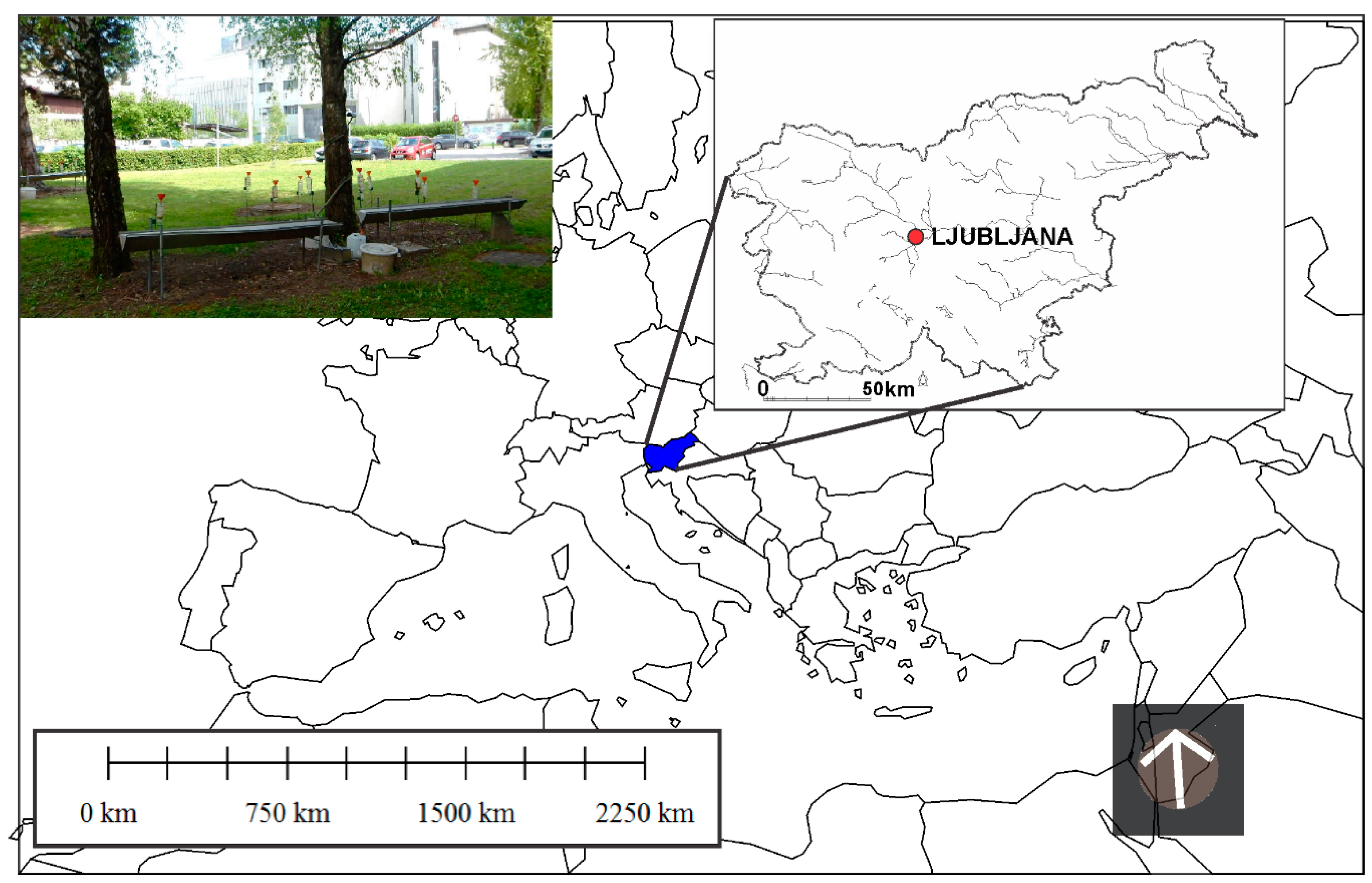
Figure 2.
Graphical presentation of the relationship among interception loss for pine trees (Ip), vapour pressure deficit and air temperature (T) (upper panel) and interception loss for birch trees (Ib), vapour pressure deficit and air temperature (T) (lower panel). Events measured in the leafless and leafed period are indicated with red and black colour, respectively.
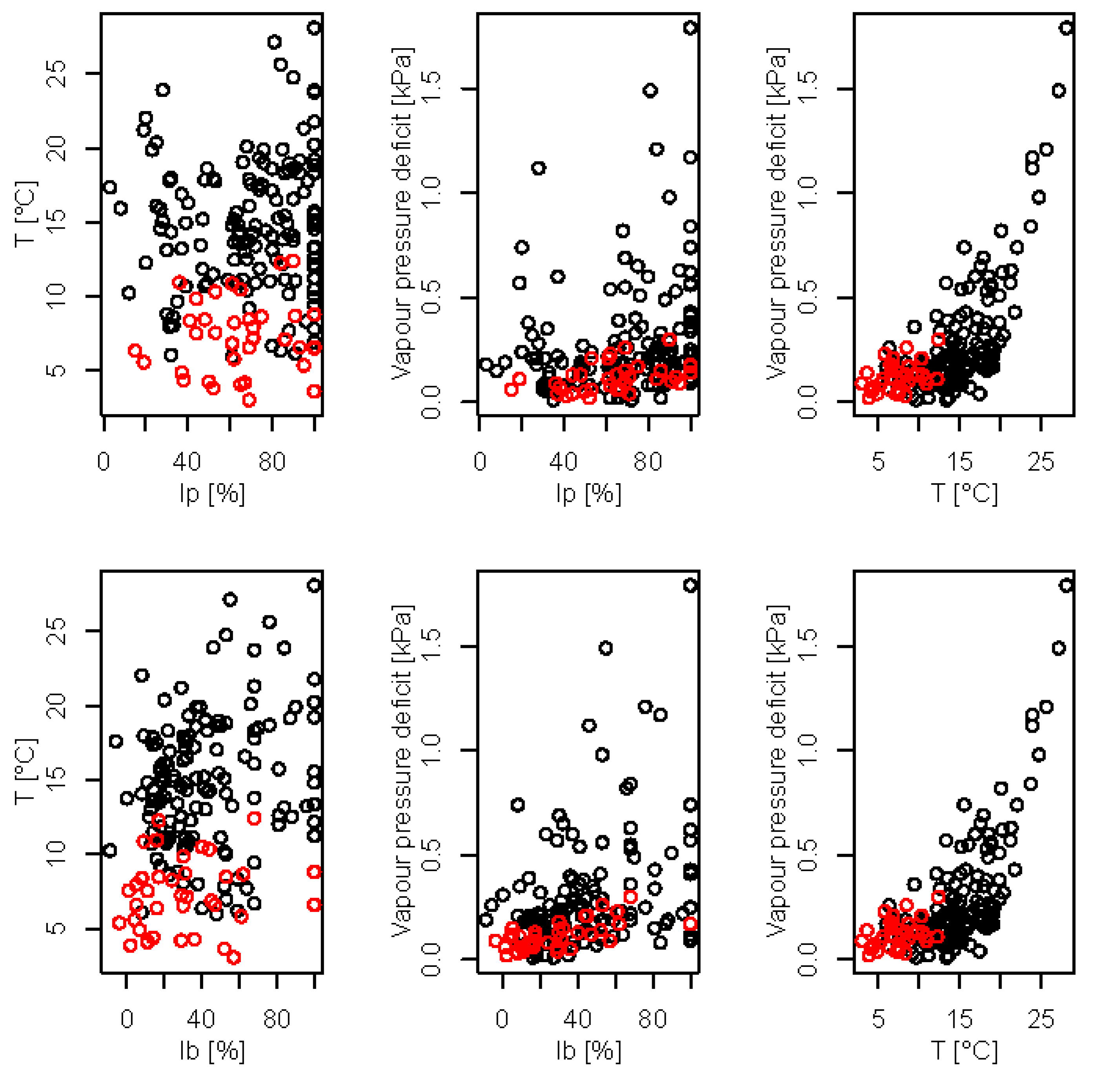
Figure 3.
Rainfall interception by birch (Ib) and pine (Ip) trees according to the amount of rainfall in the open.
Figure 3.
Rainfall interception by birch (Ib) and pine (Ip) trees according to the amount of rainfall in the open.
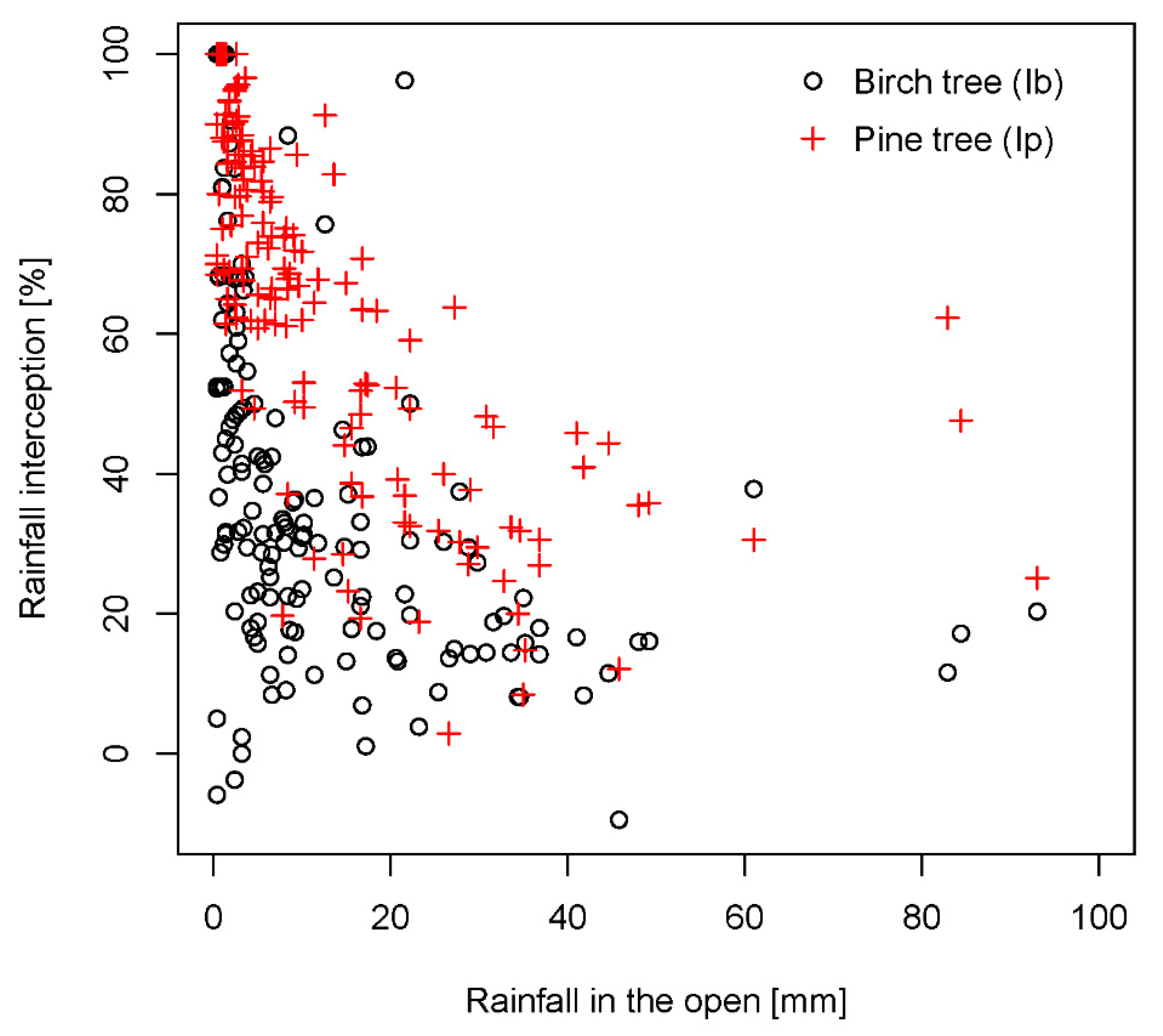
Figure 4.
Graphical fit for birch trees between measured data (red crosses) and 10,000 random realizations (grey circles) using the copula model where the Joe copula was selected as C1 and the Gumbel-Hougaard copula was selected as C2.
Figure 4.
Graphical fit for birch trees between measured data (red crosses) and 10,000 random realizations (grey circles) using the copula model where the Joe copula was selected as C1 and the Gumbel-Hougaard copula was selected as C2.

Figure 5.
Graphical fit for pine trees between measured data (red crosses) and 10,000 random realizations (grey circles) using the copula model where the Joe copula was selected as C1 and the Gumbel-Hougaard copula was selected as C2.
Figure 5.
Graphical fit for pine trees between measured data (red crosses) and 10,000 random realizations (grey circles) using the copula model where the Joe copula was selected as C1 and the Gumbel-Hougaard copula was selected as C2.

Figure 6.
Decision trees for rainfall interception by birch (a) and pine (b) trees; only the first three levels are presented. Values shown in boxes indicate mean and variance of instances related to this specific node. Numbers written outside boxes indicate values that are used to divide different nodes.


Table 1.
Definitions of the selected symmetric trivariate Archimedean copulas that were used as in Equation (6).
Table 1.
Definitions of the selected symmetric trivariate Archimedean copulas that were used as in Equation (6).
| Copula | |
|---|---|
| Joe | |
| Frank | |
| Clayton | |
| Gumbel-Hougaard |
Table 2.
Descriptive statistics (minimum, maximum, mean, median and coefficient of variation (CV)) for average air temperature (T), average relative humidity (RH), vapour pressure deficit (VPD) and rainfall interception by birch (Ib) and pine (Ip) trees.
Table 2.
Descriptive statistics (minimum, maximum, mean, median and coefficient of variation (CV)) for average air temperature (T), average relative humidity (RH), vapour pressure deficit (VPD) and rainfall interception by birch (Ib) and pine (Ip) trees.
| Variable | Min | Max | Mean | Median | CV |
|---|---|---|---|---|---|
| T | 3.0 °C | 28.1 °C | 13.4 °C | 13.4 °C | 38.5 |
| RH | 53.0% | 99.3% | 85.6% | 88.0% | 10.6 |
| VPD | 0.01 kPa | 1.79 kPa | 0.26 kPa | 0.18 kPa | 102 |
| Ib | −9% | 100% | 40% | 33% | 67.4 |
| Ip | 3% | 100% | 68% | 71% | 36.9 |
Table 3.
Kendall’s correlation coefficients between pairs of the following variables: interception loss (I), air temperature (T) and vapour pressure deficit (VPD) for birch and pine trees calculated using 175 events. p-value is shown in brackets.
Table 3.
Kendall’s correlation coefficients between pairs of the following variables: interception loss (I), air temperature (T) and vapour pressure deficit (VPD) for birch and pine trees calculated using 175 events. p-value is shown in brackets.
| Pairs | Birch Tree | Pine Tree |
|---|---|---|
| I-T | 0.16 (0.002) | 0.08 (0.10) |
| I-VPD | 0.30 (8.9 × 10⁻⁹) | 0.19 (0.001) |
| T-VPD | 0.48 (2.2 × 10⁻¹⁶) | 0.48 (2.2 × 10⁻¹⁶) |
Table 4.
Performance criteria results (root mean square error (RMSE) and mean absolute error (MAE)) for the different tested models (random sampling (n = 20, training set 75%, test set 25%) was used to calculate the results for birch and pine trees).
Table 4.
Performance criteria results (root mean square error (RMSE) and mean absolute error (MAE)) for the different tested models (random sampling (n = 20, training set 75%, test set 25%) was used to calculate the results for birch and pine trees).
| Birch Tree | Pine Tree | |||
|---|---|---|---|---|
| Model | RMSE [%] | MAE [%] | RMSE [%] | MAE [%] |
| Copula | 24.21 | 18.16 | 24.95 | 19.62 |
| Exponential function | 24.70 | 19.62 | 24.64 | 20.27 |
| Multiple regression model (MLR) | 25.29 | 20.14 | 24.94 | 20.58 |
| Decision tree | 26.92 | 20.88 | 27.75 | 22.11 |
© 2018 by the authors. Licensee MDPI, Basel, Switzerland. This article is an open access article distributed under the terms and conditions of the Creative Commons Attribution (CC BY) license (http://creativecommons.org/licenses/by/4.0/).
Share and Cite
MDPI and ACS Style
Bezak, N.; Zabret, K.; Šraj, M. Application of Copula Functions for Rainfall Interception Modelling. Water 2018, 10, 995. https://doi.org/10.3390/w10080995
AMA Style
Bezak N, Zabret K, Šraj M. Application of Copula Functions for Rainfall Interception Modelling. Water. 2018; 10(8):995. https://doi.org/10.3390/w10080995
Chicago/Turabian StyleBezak, Nejc, Katarina Zabret, and Mojca Šraj. 2018. "Application of Copula Functions for Rainfall Interception Modelling" Water 10, no. 8: 995. https://doi.org/10.3390/w10080995
Note that from the first issue of 2016, this journal uses article numbers instead of page numbers. See further details here.