Change and Climatic Linkage for Extreme Flows in Typical Catchments of Middle Tianshan Mountain, Northwest China


1
College of Resources and Environment Sciences, Xinjiang University, Urumqi 830046, Xinjiang, China
2
State Key Laboratory of Desert and Oasis Ecology, Xinjiang Institute of Ecology and Geography, Chinese Academy of Sciences, Urumqi 830011, Xinjiang, China
*
Author to whom correspondence should be addressed.
Water 2018, 10(8), 1061; https://doi.org/10.3390/w10081061
Submission received: 5 July 2018
/
Revised: 6 August 2018
/
Accepted: 8 August 2018
/
Published: 10 August 2018
(This article belongs to the Section Hydrology)
Abstract
:Due to an absence of an essential daily data set, changing characteristics, and cause of flow extremes in the Tianshan Mountains are rarely explored in depth. In this study, daily based long-term meteorological and hydrological observation data were collected in four typical watersheds in the middle Tianshan Mountains; Manne-Kendall trend analysis and Pettit’s test were used to detect the trends and alterations of extreme flow series; Generalized Extreme Value distribution (GEV) and General Pareto distribution (GDP) models were used to describe the probability distributions of annual maximum (AM) and peaks over threshold (POT) series based on daily discharge; and the relationship between extreme flow and climate indices, were also investigated. The findings indicated that, change of the AM series at five hydrological stations experienced positive trends; the POT series generally showed no significant trends, while the peaks over threshold number (POTN) present a positive trend at the five stations. Change points exist in the POT and occurrence time of maximum daily discharge in spring (AM-SPR) series at the Kensiwate (KSWT) station in Manas watershed; the mean extreme flow decreased after 1986, and the occurrence time the annual maximum daily flow in spring significant forward after 1978. The AM series can well fit the GEV distribution, while the POT series fit the GDP distribution better; the GEV model performed worse in estimating flood events with high return period than low return period events. Moreover, acceleration of glacier melting lead to the magnitude and frequency increments of flood in the north slope; intensifying and frequent precipitation extremes are dominate factors of extreme flow variations in south slope watersheds which without large amount of glacier coverage; and continually temperature rising in spring and increased precipitation in winter lead to the change on magnitude and timing of spring extreme floods.
1. Introduction
In inland river basins, usable water resources for downstream were largely influenced by temperature and precipitation changes in mountain regions [1]. Climate changes would accelerate regional hydrological cycles, and have large impacts on the formation and development of extreme hydrological events [2]. Particularly in northwest China, almost all rivers are fed by snow and glacier melting water from mountain regions [3]. The cold indices decreased significantly, and the warm indices increases had significant, and precipitation in mountainous regions had presented increase trends during past decades [4]. Moreover, previous researches have shown that the flood risk increased in several typical river basins of the northwest China [5,6]. The increments of flood magnitude and frequency have causing serious damages to the national economy, and to arable land and properties in the region [7]. Scientific understanding of changing characteristics extreme flood and analysis of the response of climate change are key problems in flood control, hazard warning, and the water allocation in arid and semi-arid inland river basins [8].
Tianshan Mountains are located in the center of the Eurasian continent, across Xinjiang of China, and extending westward to Kyrgyzstan [9]. The total length the mountains is about 2500 km, with an average width of 250–350 km. The Chinese Tianshan Mountains, is about 1700 km in length and is located in the territory of China covering an area of more than 570 × 103 km2, and accounting for about 1/3 area of the Xinjiang Province. Xinjiang is divided into two parts by the mountains; the north is the Junggar basin and the south is Tarim Basin. Rainfall and snowfall in the Tianshan Mountains is relatively rich because the mountains block the uplifting air currents from the Atlantic and Arctic [10]. In fact, 65% of the surface streamflow in Xinjiang rise in these mountains, and provide agricultural and domestic water for the surrounding basins and oases. Moreover, the mountains have abundant extant glacier and snow covers, and are so called as the “water tank of Central Asia” [11]. As the most important fresh water supply, total contribution of glacier melt water to the river flow was estimated to be about 10% at the outlets of Tianshan Mountain valleys, and this value reached 50% in the Tarim Basin [12]. Many reports have shown a significantly climatic change in the Tianshan Mountains during the past 60 years [1,5]. Since the 1950s, the temperature presented a significant rising trend (significance level is smaller than 0.001) with a rate of 0.33–0.34 °C/10a. Precipitation increased substantially in most regions especially for the middle and high latitudes. Glacier area decreased by 11.5% and the thickness of snowpack has also decreased. Pan evaporation and wind speed have also changed [9].
With climate change of the Tianshan Mountains, hydrological processes in such mountainous watersheds have drawn great attention from researchers. There is a number of studies that make efforts to address changing properties of stream flow [13,14,15,16,17]. Ding et al. [13] investigated the trend glacier change under climate change, and indicated retreat of glacier and increased glacier-melting runoff. Chen et al. [15] and Xu et al. [16] indicated that both the precipitation and temperature had increased in the upstream catchments of Tarim River in the middle of the 1980s. The increase of temperature in the Kaidu and Aksu watersheds is higher than that in the Yarkand Hotan watersheds. The runoff at Aksu River is significantly increased in recent 50 years, and the annual runoff had increased by 10.9% since 1990. Ling et al. [17] indicated that the precipitation, air temperature, and runoff in Tarim headstreams increased during both high-flow and low-flow periods; both climate change and human activity had remarkable effects on the total runoff during the period of the 1990s and 2000s, and climate change was the major driving factor of flow variation during high-flow periods. Kong et al. [18] found that, during the 48 years of observation records in the Urumqi River, temperature has less impact on river discharge than precipitation. Deng et al. [1] investigated that climate change in mountainous region will have seriously effects on water resources condition in inland river basins. Generally, previous studies on the hydrology of mountainous watersheds are mostly focused on the average state of stream flow. Historical data also indicate climate change over the last few decades and human activities in high elevations is likely to initiate more flood or drought extremes and led to flow regime alteration [19]. However, changes of extreme flows in the Tianshan Mountains are have rarely been investigated due to absence of essential daily data set [20].
In this study, daily based meteorological and hydrological records at four typical watersheds in the middle part of Tianshan Mountains were collected; multi-statistical methods (i.e., Manne-Kendall trend analysis and Pettit’s test) and frequency analysis models were used to investigate the changes of extreme flows on magnitude, timing, and frequency. The study is aimed to: (1) analyze the trends and alterations of the stream flow extreme series; (2) fit the extreme flow series by using Generalized Extreme Value distribution (GEV) and General Pareto distribution (GDP), and evaluate the performances of the models; and (3) understand the relationship between selected climate indices and the extreme flow changes. The results obtained will be used for helping local officials to establish effective flood control and hazard warning policies, and thus improve the local water resources security.
2. Study Area and Data
The middle part of Chinese Tianshan Mountains (MCTM) is located between Latitude 41.06°–39.40° N and Longitude 86.61°–88.50° E, with an area of 156 × 103 km2. Mean annual precipitation is around 300 mm in the mountain region, and 70% of which occurs from June to October. The mean annual temperature is around −5 °C. Pan evaporation is approximately 1157 mm/year, and the average actual evapotranspiration is approximately 216 to 363 mm/year for different land-cover types [5]. It supplies water for agricultural, municipal, industrial, and ecological environments of the oasis, with an area of over 85,000 km2 and a population of over 2.05 million; and also the main water source for the core city group of Xinjiang Uygur Autonomous region, which include the cities of Urumqi, Shihezi, Korla, etc. Flood or drought extremes would lead to serious damages and losses, especially in densely populated cities and villages and/or ecologically fragile areas [18]. Therefore, it is important to evaluate the impacts of climate change on the main rivers and investigated the mechanism of extreme flows variation in the middle Tianshan Mountains.
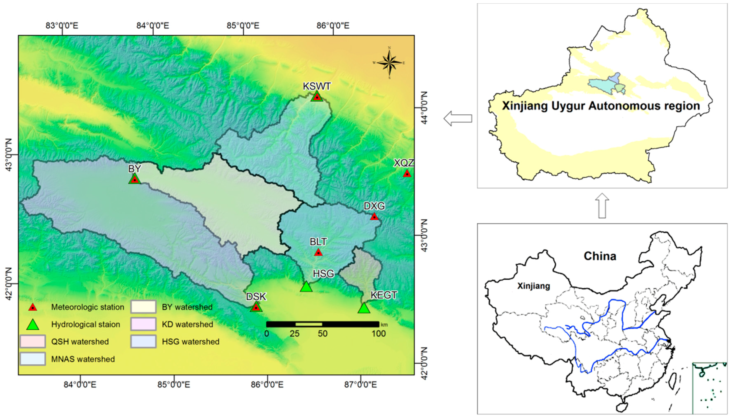
Four typical river basins were selected for investigating the changes of extreme flood, which include Manasi watershed in the north slope of Tianshan Mountains, Kaidu, Huangshui, and Qingshui watersheds in the south slope of the mountains. In this study, historical daily discharges at five hydrological stations in the MCTM are selected to analyze changing properties of streamflow extreme events. The Kaidu River is represented by Dashankou (DSK) station, while Bayblk (BY) station controls the upstream sub-watershed in the northeast part of the Kaidu watershed. The Manasi River is represented by Kensiwate (KSWT) station. The Huangshui River and Qingshui River are represented by Huangshuigou (HSG) and Kerguti (KRGT) stations, respectively. Correspondingly, observed meteorology data at Six weather stations include Bayblk (BY) and Dashankou (DSK) stations which are located in the Kaidu watershed, Kensiwate (KSWT) station which is located in the Manasi watershed, Baluntai (BLT), Daxigou (DXG) stations which are located in the Huangshui watershed, and Xiaoquzi (XQZ) station which is nearby the Manas and Huangshui watersheds. Daily precipitation, daily mean temperature, and snow depth at the six meteorological stations are collected. Figure 1 presents the hydrological and meteorological stations.
3. Data and Methodology
3.1. Data Collection and Preprocessing
Table 1 lists the location, drainage area and data interval of the five hydrological stations in the study area. Data were collected from the Xinjiang Hydrology Bureau and the Xinjiang Tarim River Basin Management Bureau, China. Data quality is controlled before it is used, and the method proposed by Ding et al. [13] is used to make up the missing data. For DSK and KSWT hydrological stations, there are some missing values in the daily runoff data series at the 2 stations during 1958–2011. For BY, HSG and KRGT hydrological stations, it is difficult get the complete sequence of daily runoff data over 50 years; and the research periods were identified as 1978–2011, 1958–1989 and 1958–1989 according to the available data sets, respectively.
The analysis is based on the sample sequences selected via annual maximum (AM) method and peaks over threshold (POT) method. AM method is the standard method of flood calculation specification, and have been wildly used in the engineering design and experimentation [20,21]. However, extreme runoff information in AM series is limited, and the annual maximum runoff only has relative significance. The POT method can greatly increase the sample size, to maximize the use of useful extreme information and solve the lack of observation hydrological data. Percentile value method, mean excess plot method, goodness of fit test and bootstrap method are most commonly used methods to selected POT series [22]. Willems [23] presented a method where peak flows are selected from the flow series based on criteria for the inter-event time, the inter-event low flow discharge and the peak height. Two subsequent events in selected flood extreme series can be considered nearly independent when following conditions are satisfied:
- (1)
- the time length t of the decreasing flank of the first event exceeds a time kp, t > kp;
- (2)
- the discharge drops down—in between the two events—to a fraction lower than f of the peak flow; where qmin, qmax, and qbase would be the minimum discharge, the maximum discharge and the base flow, respectively:
- (3)
- the discharge increment from to has a minimum height , . This procedure for peak flow selection has three parameters: kp, f and . It is based on the concept that a peak flow event can be considered largely independent from the next one, when the interevent discharge drops down to a low flow condition or almost to the baseflow level (see criterion (2)). Under this condition, the quick flow components attributed to the peak flow events are indeed nearly independent.
Besides of the AM and POT series, other six series represent the extreme flow variation include spring maximum daily flows (AM-SPR), maximum daily discharge in summer (AM-SUM), occurrence time of annual maximum daily discharge (AMT), occurrence time of maximum daily discharge in spring (AM-SPRT), occurrence time of maximum daily discharge in summer (AM-SUMT), and annual peaks over threshold number (POTN) were also extracted at the five hydrological stations.
In addition, daily precipitation, air temperatures and snow depth at the BY, DSK, KSWT, BLT, DXG and XQZ stations in the period from 1961 to 2010 were used. Several indices were extracted for climate linkage analysis, such as annual or seasonal precipitation, annual maximum snow depth, yearly and seasonal mean temperature and active accumulated temperature. For extreme rainfall events, annual/seasonal maximum of precipitation (AMP) were generated via AM method; and the data of the daily precipitation observation data over the 99.5th quintiles are selected to make up the peaks over threshold of precipitation (POTP), while peaks over threshold number of precipitation (POTNP) also counted.
3.2. Methods
3.2.1. Trends Analysis and Change Point Detect
Linear trend analysis and Mann-Kendall test (M-K) [24,25] were used to detect the trend of time series of hydrology and climate indices. Liner trend is normally introduced through natural or artificial changes in hydrological and metrological time series, and be used to detect shift (in decreasing and increasing direction) in hydrometeorological time series and to describe possible generating processes underlying a given sequence of observations [2]. And as a nonparametric test method, the M-K is used to verify whether trends are significant; and also can process missing data and extreme. The results of the Mann-Kendall test were heavily affected by the serial correlation of the time serial correlation, so Yue and Pilon method [26] was adopted to deal with the correlation among series.
Assuming an observed time series x1, x2, …, xn, corresponding to the time series t1, t2, …, the statistical value S of the M-K method is:
When n ≥ 10, the S value of the M-K test is similar to a normal distribution, with a mean of 0. The variance is:
The Z value is used to evaluate whether the time series data presents a significant trend. The Z value is defined as:
indicates that, there is a significant trend in the sample sequence. A negative (positive) value of S indicate a significant downward (upward) trend. is the significance level, and the varying correspond to varying . In this study, 0.05 is set as the significance level, making . If the , the time series shows a significant downward or upward trend.
Change points of the time series were detected by Pettit’s Test [27], and this approach is commonly used for detecting a single change-point in continuous time series. It tests the H0: the T varibles follow one or more distributions that have the same location parameter (no change), against the alternative: the time series has a change point.
where
The is the change-point of time series, provided that the statistic is significant. The significance probability of is approximated for with:
3.2.2. Frequency Analysis
In the 1930s, Fisher and Tippett [29] put forward three extreme value distributions in the study of the maximum asymptotic distribution theory, which are the Gumbel distribution, Fréchet distribution and Weibull distribution. According to extreme value distribution theory, Jenkinson [30] and Coles [31] unified the three extreme value distributions as an extreme value distribution with three parameters, which is the generalized extreme value distribution (GEV). The probability density function (PDF) of the GEV distributions given as follows [2,23]:
where is the scale factor, is the location factor, and is the shape factor. The GEV distribution includes the Weibull distribution ( < 0), Gumbel distribution ( = 0) and Frѐchet distribution ( > 0).
Another distribution used in this paper is General Pareto distribution (GDP), and it is the POT stable distribution. The GDP filter extreme data according to a given threshold, and then establishes extreme value distribution. The distribution function of GDP is given as follows [32]:
where is the scale factor, is the location factor, and is the shape factor. The GDP distribution includes the exponential distribution ( = 0), Pareto distribution ( > 0), and Weibull distribution ( < 0).
There are many methods for parameters estimating in extreme distributions, such as moments method, probability weighted moments method (PWM), L-moments method, Bayes estimation method and maximum likelihood estimation method (MLE), and so on. Each parameters estimating method has its strengths and weaknesses, but MLE is the approach of best versatility of all, which can adapt to different parameters estimating of extreme models. MLE is put forward by British statistician R.A. Fisher in 1912 [33]. Because it can be used for every population and has good asymptotic property in the case of large sample, it becomes one of the most commonly used and most important methods for parameters estimating. The estimates obtained via MLE have consistency and effectiveness. If not unbiased, it can be modified to be unbiased. Under certain conditions, difference between maximum likelihood estimation of the unknown parameters and its true value can be made arbitrarily small. MLE method is a good, easy to be adaptable to complex models, so parameters were estimated through MLE method. In the approach, data samples in the time series are independent and identically distributed with the probability distribution function F(x). The parameters estimation of GEV by MLE is described as follow:
where ; point (σ,ξ) reaches the MLE when the function reaches the maximum point. There is no analytical expression of μ,σ,ξ, so numerical methods are needed to solve the function [28].
The return period (i.e., average time between two independent events) is an important parameter for studying hydrological extreme problems. It describes the probability of extreme occurrence and temporal dimensions, and can be used as a measure of safety (the ‘inverse risk’). Based on the method of GEV, the return period is calculated as follow:
For GPD, return periods of the estimation of extreme runoff can be calculated as follows:
3.2.3. Pearson Correlation Analysis
Pearson’s correlation coefficient is usually applied in measuring the relationship between random mathematical variables or observed time series [34,35]. It was used to calculate the correlation between extreme flow series and climate change indices. The Pearson’s correlation coefficient can be calculated as follows:
where is Pearson’s correlation coefficient and and are the values of measured datasets. The correlation coefficient is between −1 and +1 [36]. The values of −1 indicate a perfect inverse linear relationship; values of +1 indicate a perfect direct linear relationship; when the value approaches zero, two data series close to uncorrelated.
4. Results and Discussions
4.1. Trends and Alterations of the Extreme Flow Series
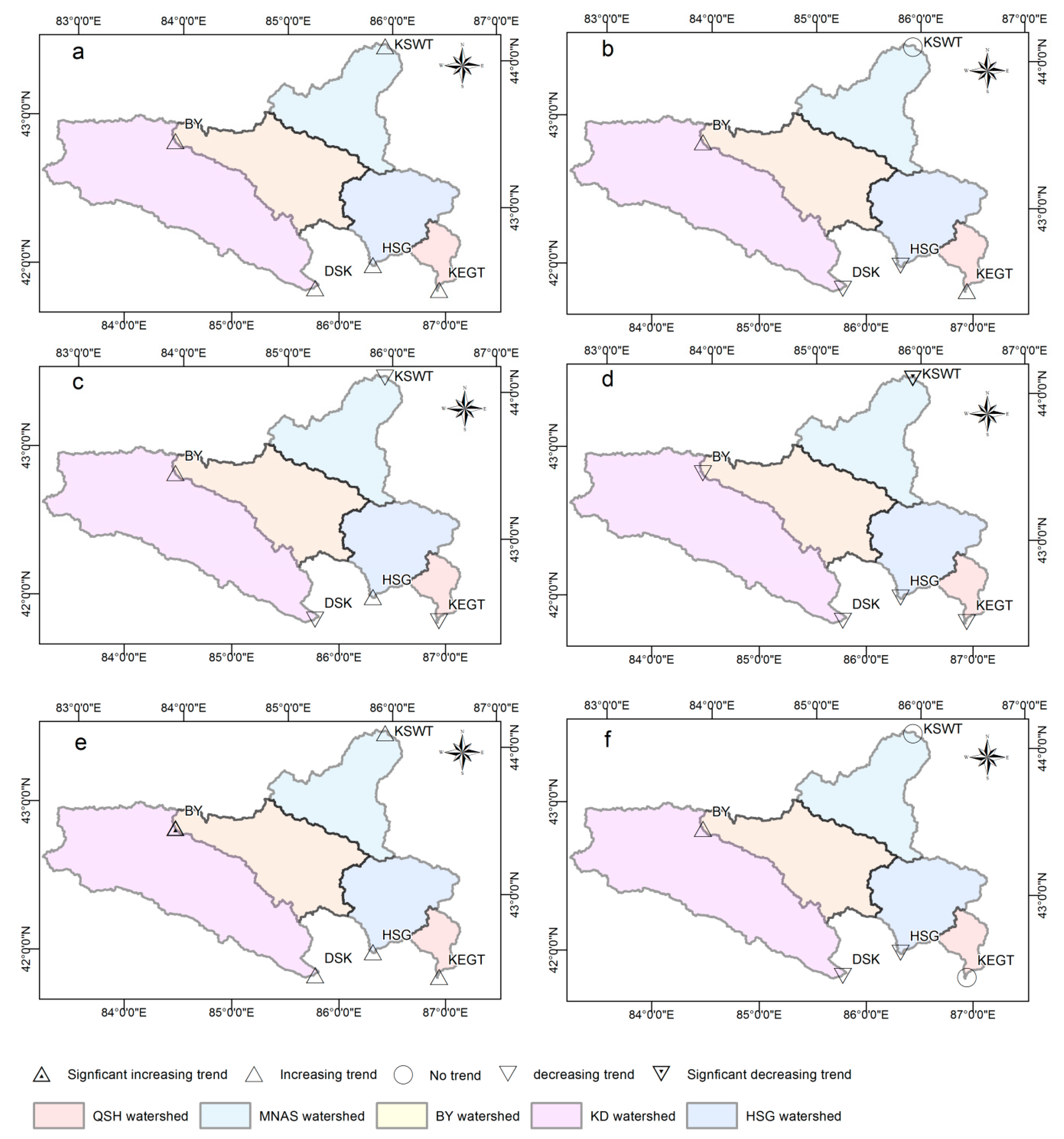
Linear trend, the M-K test and the Pettitt’s test approach were conducted to analyse the trend and alteration of the extreme flow series. Figure 2 shows the trend analysis results of annual and seasonal maximum daily flows, as well as the occurrence time of them. The results indicated that, AM series at five gauging stations show an increasing trend; AM-SPR series at two gauging stations (i.e., BY station in Kaidu watershed and HSG station in Huangshui watershed) show an increasing trend, while those at the other three AM-SPR series show a decreasing trend (i.e., DSK station in Kaidu watershed, KSWT station in Manas watershed and KRGT station in Qingshui watershed); AM-SUM series, all five stations show an increasing trend. At the BY station which located in the upstream of the Kaidu River, summer maximum daily flows (AM-SUM) showed a significant increasing trend at the significance level of 0.05; and p value which represent the statistical significance is 0.043 when tested by the M-K method. Moreover, the occurrence time of extreme flow events shift to an earlier date, particularly for the AM-SPRT. All five AM-SPRT series show negative trends during research periods, but only exhibiting a significant forward trend at the significance level of 0.05 in KSWT station with the p values of 0.011.
In addition, POT series of five gauging stations in four study watersheds did not show significant trends, while the annual POT number (POTN) are mainly increased. Especially at DSK station in the Kaidu watershed, the increase trend of POTN is significant for p value less than 0.05 (Figure 3).
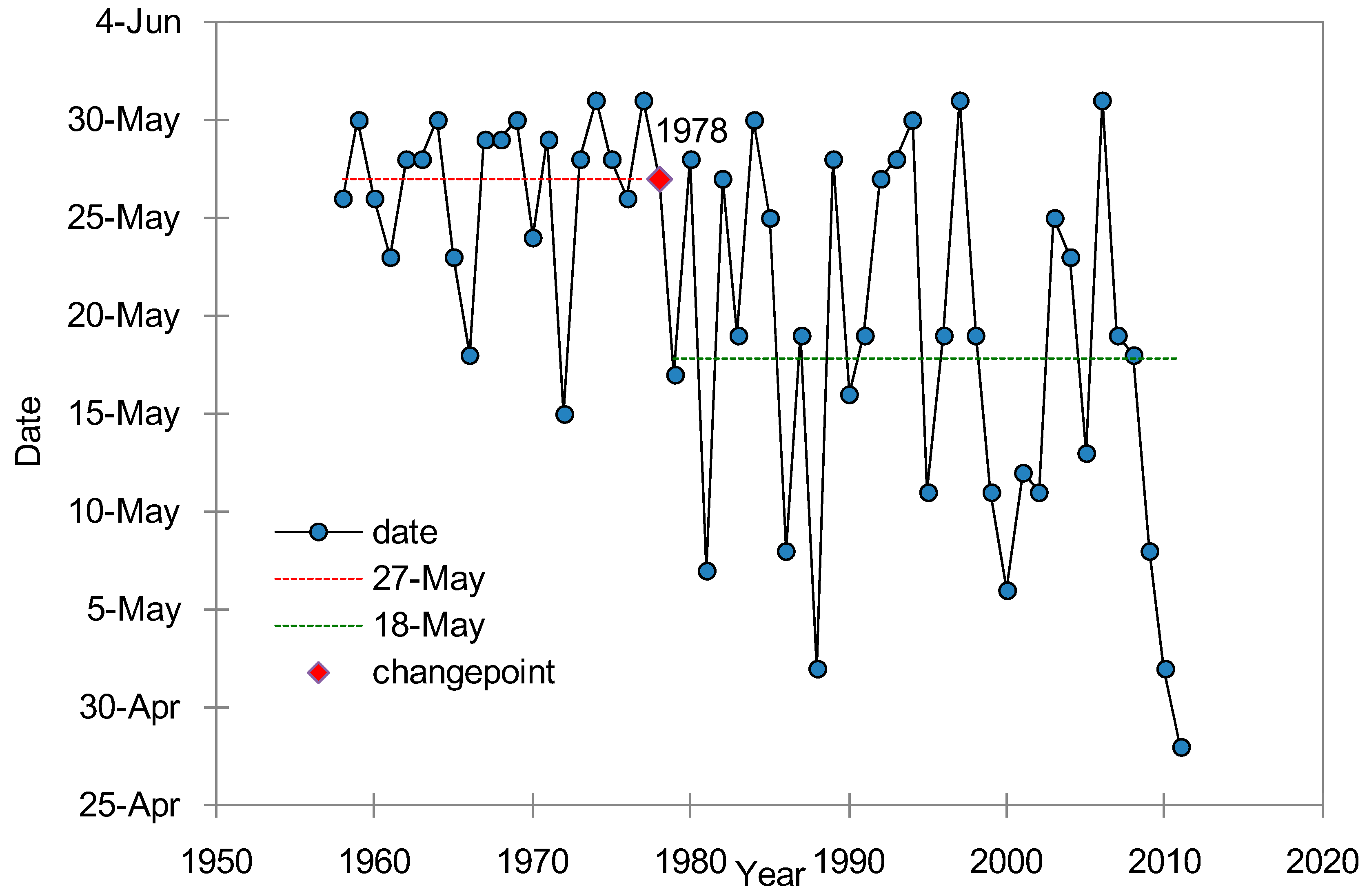
The Pettitt’s test was conducted to check the change points (Table 2). Among the eight kinds of time series for extreme flows, change points only exist in the POT and AM-SPRT series. For POT, change points at the KSWT station in Manas watershed occurred in 1986 with a p value of 0.039 (i.e., the change point is significance at a significance level of 0.05), and the mean daily discharge before and after the change point were 221 m3/s and 325 m3/s, respectively (Figure 4). Mean extreme flow decreased after 1986, and the discharge decreased by 33.1%. For AM-SPRT, change points of the KSWT station in Manas watershed occurred in 1978 with a P value of 0.004 (i.e., the change point is significance at a significance level of 0.01), and the mean occurrence time before and after the change point were 27 May and 18 May, respectively. The occurrence time the annual maximum daily flow in spring significant forward after 1978.
4.2. Extreme Event Analysis
Parameter estimation and the goodness-of-fit test results are listed in Table 3. The GEV distribution fit better for the AM series, while the GDP distribution fit better for the POT series. There are four of the five AM series that pass the K-S test with a significance level of 0.05. Among them, the AM at KSWT and DSK stations can fit well the Frѐchet distribution in GEV, and the AM at HSG and KRGT stations fitted the Gumbel distribution. However, the K-S test statistics of the AM at BY station was 0.258, which was greater than the threshold value under 0.05 significance level but pass the K-S test with 0.01 significance level. For POT, there are three of the five series pass the K-S test with 0.05 significance level, and one series pass the K-S test with 0.01significance level. The POT at KSWT, DSK, HSG, and KRGT stations can fit well the Pareto distribution in GDP. The POT at BY station can fit the Exponential distribution in GDP, but the K-S test statistics were 0.336, which was greater than the threshold value under 0.05 and 0.01 significance levels. Moreover, the PPCC test statistics are above 0.9, which indicates that the observation samples are highly correlated with the theoretical distribution for all AM and POT series.
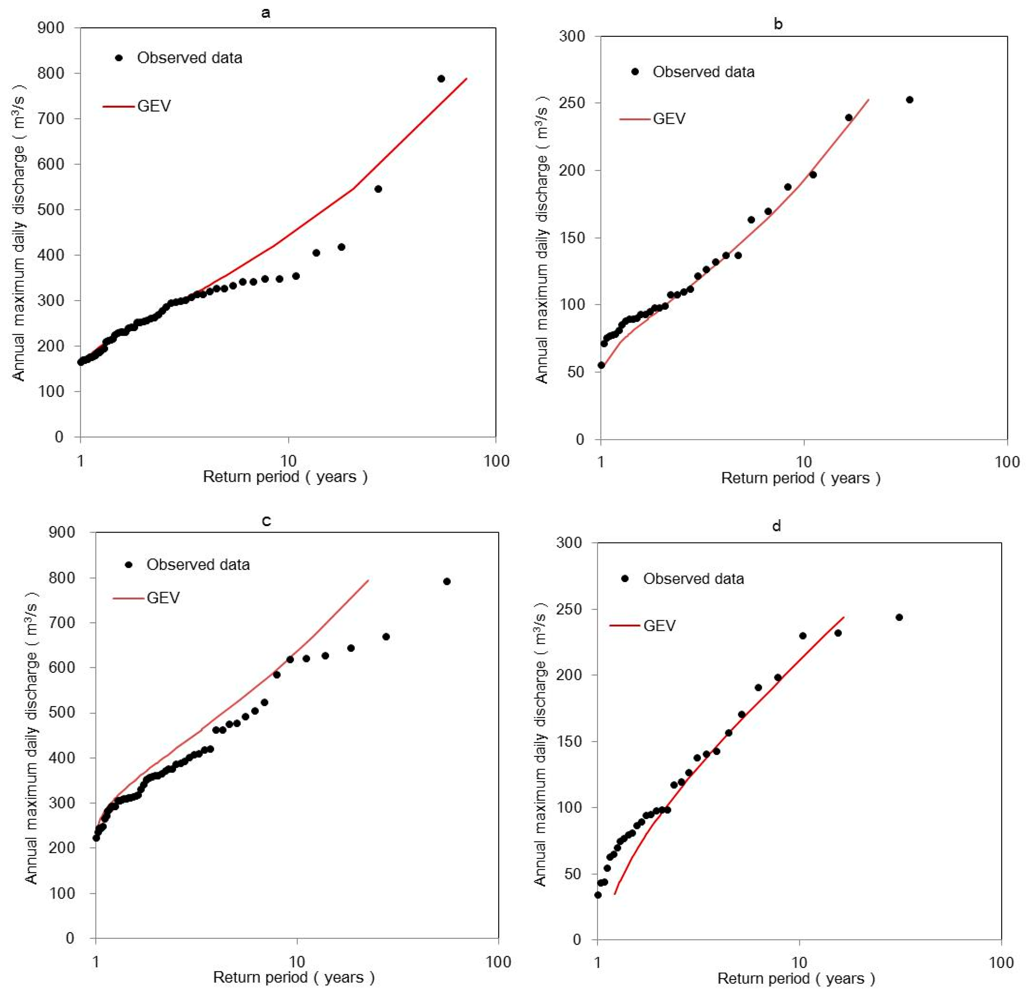
The GEV fitted lines of the five stations match the measured annual maximum daily discharge, indicate that the GEV distribution can modeling the observed data trend of AM series (Figure 5). The GEV model fitted errors on AM for 5 year, 10 year, 20 year, and the longest records at each hydrological station are shown in Table 4. The results indicated that, the estimate errors of the AM ranges from −0.5% to 27.2%; and the GEV fitted lines generally match well with observations at the lower end, and overestimate peak flows at the high end. For the return period of 5 year, the fitted lines fit the observations well at the BY, DSK, HSG, and KRGT stations with only −0.7%, 2.1%, −0.5%, and 5.9% errors, respectively; while the estimated error at the KSWT station is 9.1%. This show that GEV performances better in fitting low return period events in the south slope watersheds than that in the north slope watershed of middle Tianshan Mountains. For the longest return periods, the maximum recorded AM is 789 m3/s and the GEV fitted line is 721 m3/s at the KSWT station, which leads to the error of −8.6%; however, the errors of the GEV predictions at the BY, DSK, HSG, and KRGT stations are 13.0%, 18.5%, 14.8%, and 18.1%, respectively. The GEV performances worse in estimating high return period events than low return period events at both north and south slope watersheds.
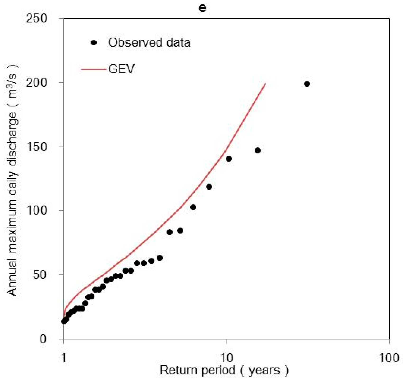
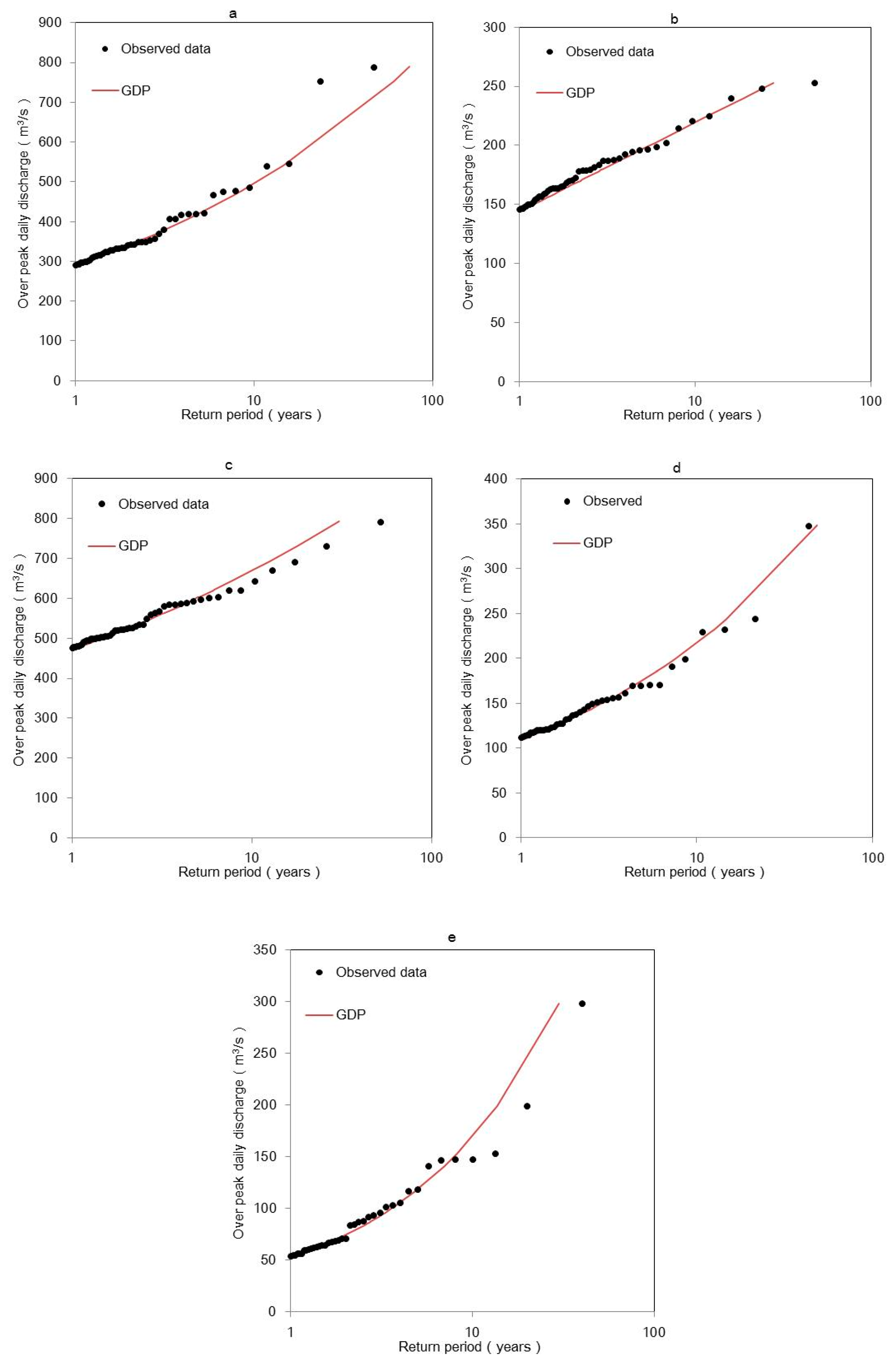
As shown in Figure 6, the GDP fitted line generally matchs better with observations than that of the GEV model, and the estimate errors of the POT ranges from −0.5% to 23.6% (Table 5). For estimating peak over discharges for 5 year return period, the GDP model fitted line fits well with the observation, and the errors are within . However, in fitting maximum peak over discharges that correspond to the return periods of 31 to 54 years at the different stations, the GDP overestimate the extreme flood with 7.9%, 4.7%, and 23.6% at the BY, DSK, and HSG stations; but underestimate the flood discharges with 8.7% and 4.5% at the KSWT and KRGT stations, respectively.
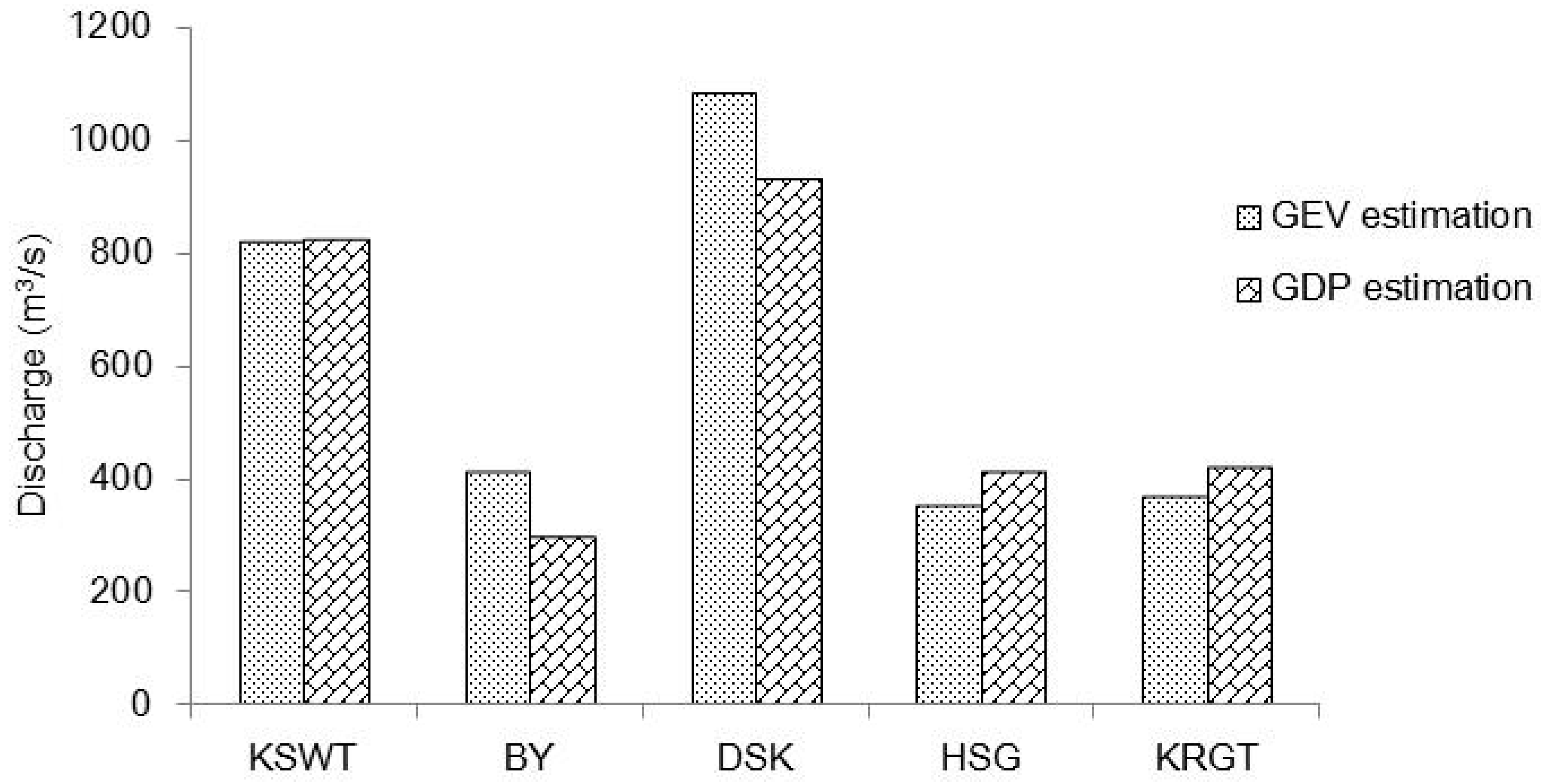
Figure 7 shows the GEV and GDP estimations for design floods of 100 year return period. The results indicate that, 100 year design flood predicted by GEV model are 816 m3/s, 410 m3/s, 1080 m3/s, 350 m3/s, and 365 m3/s at the KSWT, BY, DSK, HSG, and KRGT stations, respectively. The GDP predicted discharge are higher than those of GEV at the KSWT (820 m3/s), HSG (410 m3/s) and KEGT (416 m3/s) stations, while lower than those of GEV at the BY (292 m3/s) and DSK (930 m3/s) stations.
4.3. Discussion of the Linkages between Extreme Flow Change and Climate Factors
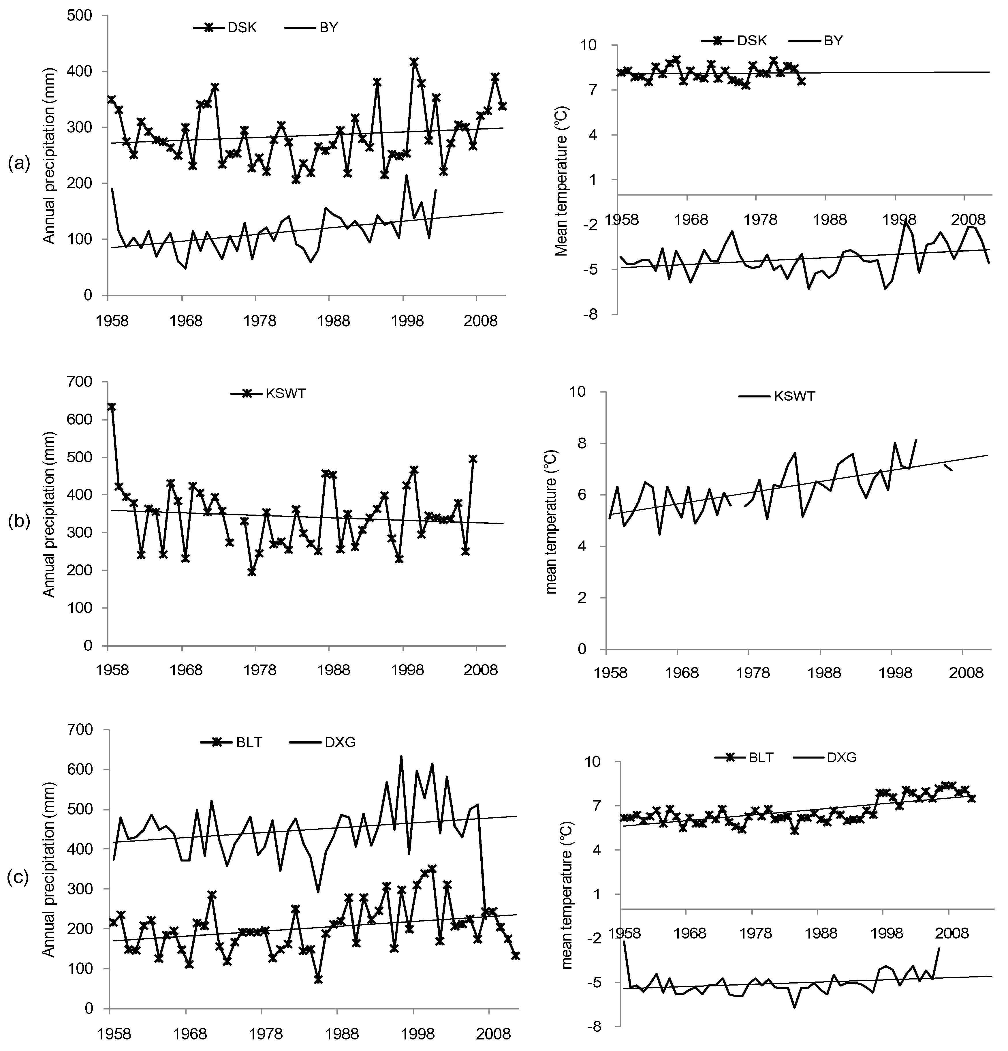
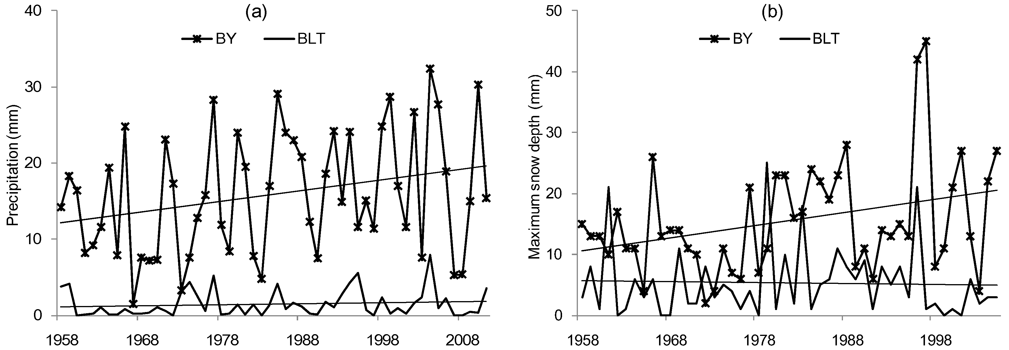
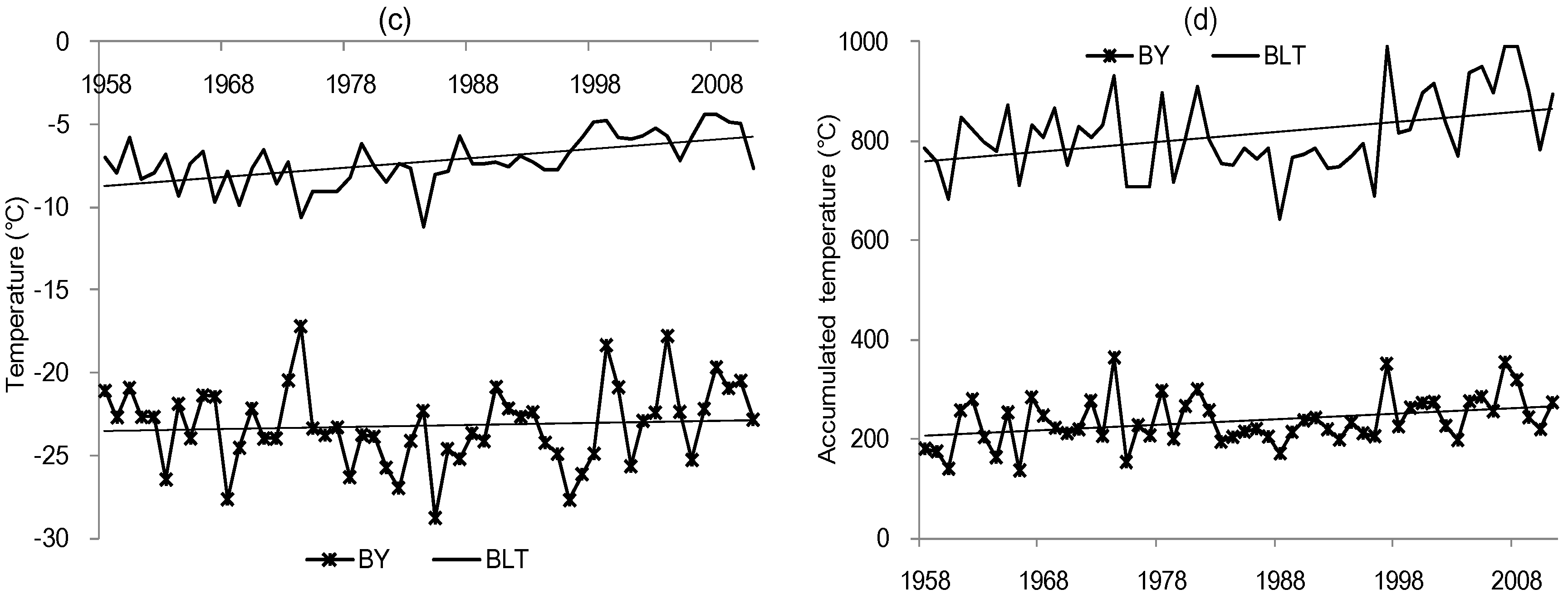
Changes of flood in both time and space are the result of climate change and human activities [28]. However, in the Tianshan Mountains, the interference of human activities in the alpine region is relatively small, climate change is usually considered to be the main driving factors of hydrological alterations [37]. Since the 1950s, the annual average temperature in the Tianshan Mountains has been rising with an increase rate of 0.34 °C/10a, which is slightly higher than the mean temperature of the whole region (i.e., 0.32 °C/10a), and much higher than warming rate of the global (i.e., 0.13 °C/10a) [5,38]. Moreover, the precipitation increase rate is 15.5 mm/10a in the Tianshan Mountains, and it is the region with the increasing trend of precipitation in Xinjiang [7]. In the middle of the Tianshan Mountains, five meteorological stations (i.e., BY, DSK, KSWT, BLT, and DXG) located in the four typical watersheds (i.e., Kaidu, Manas, Huangshui, and Qingshui). As shown in Figure 8, annual mean temperature in the all six stations increased during the research periods. When tested by the M-K method, the series present significant increase trends at the significance level of 0.05, and the p values are 0.010 and 0.035 at the DXG and BY station, respectively. At the XQZ, KSWT, and BLT stations, the annual mean temperature series are significantly increased at the significance level of 0.01, with the p value of 0.004, 0.001, and 0.001, respectively. However, the changes of precipitation have not shown a consistent trend in different stations. Annual mean precipitation in BY, DSK, BLT, and DXG stations showed an increase trend during the research period, while it showed a decrease trend in KSWT station. The long-term trends are significant for precipitation at the significance level of 0.05 in DSK with a p value of 0.02, and at the significance level of 001 in BLT with a p value of 0.02. The largest increase rate is 20.1 mm/10a which were found in DSK station. In general, the trend of climate change in the typical watersheds at the middle Tianshan Mountains is consistent with the general conclusions of Xinjiang and Tianshan Mountains, but the change range is different [39].
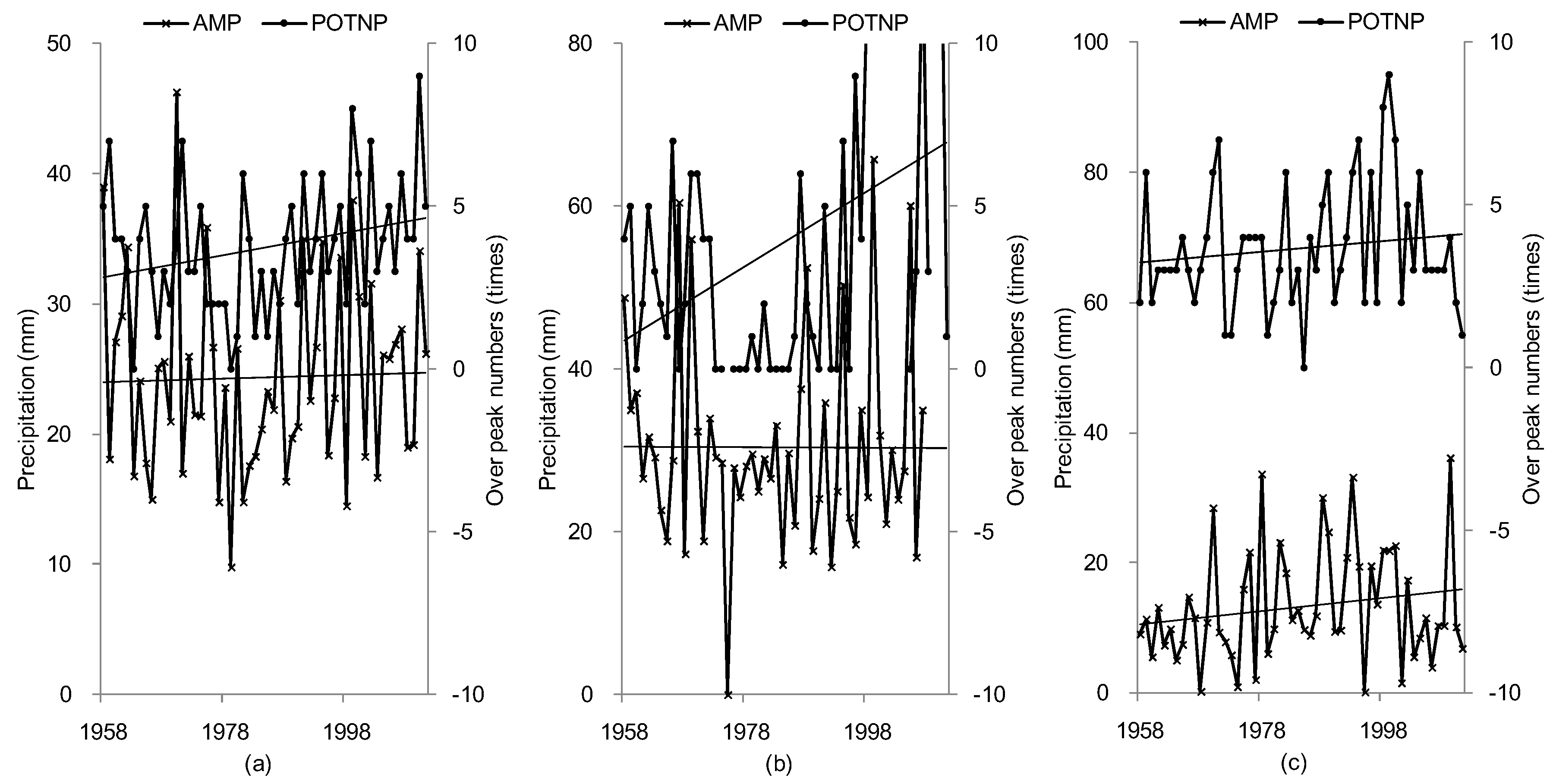
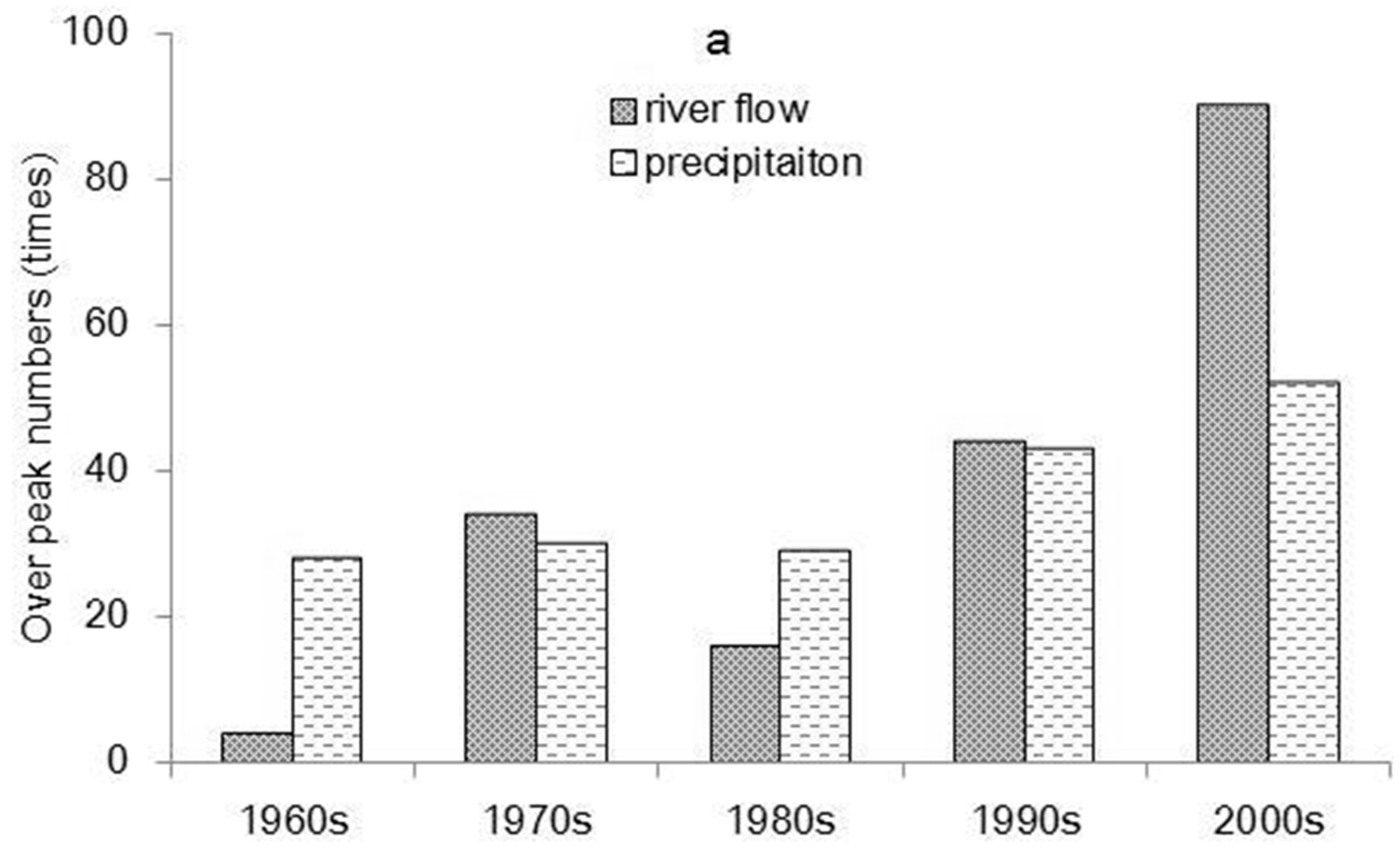
Qian et al. [40] indicated that, the increase of intensity and duration of precipitation has an important contribution to the flood frequency increment in Tianshan area from 1980 to 2000. And Mao et al. [19] presented that annual maximum peak discharge has been increased in Tuoshengan River, Kumalake River, Manas River, and the Urumqi River’s which originated in the Tianshan Mountains over the past 50 years; and it may be related to the increase of glacier ablation and rainstorm intensity in summer. In this study, magnitude and frequency variations of the extreme rainfall events in typical watersheds were analyzed. As shown in Figure 9, annual maximum daily precipitation in the Manas watershed did not change obviously, and slightly increase in Kaidu, Huangshui, and Qingshui watersheds. However, the numbers of over peak rainfall events were obviously increased for all research watersheds. On the other hand, continuous temperature rises accelerate the melting of glaciers in the alpine region. There is an interesting phenomenon that was found in the Manas watershed which is located in the north slope of Tianshan Mountains. At the KSWT station, annual and summer maximum daily discharges showed an increasing trend during 1958 to 2011, although both annual mean precipitation and summer precipitation presented a decreasing trend. Previous studies of Wang et al. [41] and Ling et al. [42] indicated that, on the northern slope of the Tianshan Mountains, glacier retreat in Manas watershed is faster than other mountainous catchments, and the glacial retreat rate ranges from 0.4%/a to 0.8%/a. Therefore, accelerated melting of glaciers which caused by temperature rise, would be the dominant factor which driving the flow extremes change in the Manasi River. For Kaidu, Huangshui, and Qingshui watersheds located in the south slope of Tianshan Mountains, where the glacier area is very small or not covered, intensifying and frequent precipitation extremes are the major driving factor triggering hydrological changes of flood events. For example, summer maximum daily precipitation at upstream meteorological station and extreme flows of the Kaidu watershed are highly related; the correlation coefficients are 0.61 between the maximum daily precipitation and the maximum daily flow, and 0.72 between the maximum daily precipitation and the maximum 3-daily flow, respectively [39]. Figure 10 presented the impact of extreme rainfall on the extreme flows, the increase of extreme precipitation events (i.e., the sum of all extreme rainfall event numbers during fixed time periods) would lead to more extreme flood events (i.e., the sum of all extreme flow event numbers during fixed time periods) in summer; and the water contribution of extreme flood (i.e., the sum of volume in all extreme flood events during fixed time periods) to total flow (i.e., the sum of daily discharge during fixed time periods) also increased. Thus, increase of extreme rainfall in summer would be dominant factors for changes of summer floods for such watershed without large amount of glacier coverage.
In addition, there is a great difference among the watersheds for spring flow responses. The results of this study indicate that, in spring, extreme flow series (AM-SPR) at the five gauging stations did not showed a uniform increase or decrease trend; while the occurrence of maximum daily discharges (AM-SPRT) at the all five stations presented earlier times within one year. Figure 11 shows the comparison of the climate factors which related to spring extreme flow in the Kaidu and Huangshui watershed. For the Kaidu watershed, both mean temperature and active accumulated temperature (>0 °C) in spring obviously increased at BY station, and the occurrence time of extreme flows at DSK station was negatively related to active accumulated temperature at BY. Winter precipitation at BY station increased with an average increment rate of 1.6 mm/10a, but the average winter temperature changes very small (Figure 11c,d); several previous works also showed increased snow accumulation provided more water reserves for spring snowmelt flood [41,42,43,44]. However, in the HS station, winter precipitation at BLT station was not changed obviously, while mean temperatures in winter have rose significantly; the snow accumulation showed slight decrease during research time. Although temperatures in spring still showed an increasing trend, the AM-SPR series at the HSG station showed a decreasing trend due to less snow melting from upstream region of the watershed. Thus, continually temperature rising in spring and increased precipitation in winter are the main reasons for the change of spring extreme flood.
5. Conclusions
This study investigates changing properties and climate linkage of the extreme flows based on long-term observation data of four typical catchments in the middle part of the Tianshan Mountains. M-K test and Pettit test were used to detect the trends and the change points of the extreme runoff series; the GEV and GDP models were applied to describe the probability distribution of extreme flows; and temporal-spatial relationship between extreme floods and climatic indices were discussed.
(1) The AM series at five gauging stations which are located in the four typical watersheds showed an increasing trend; AM-SPR series at BY in Kaidu watershed and HSG in Huangshui watershed showed an increasing trend, while other AM-SPR series showed decreasing trends; AM-SUM series at all stations showed an increasing trend. Moreover, AM-SPRT series generally showed forward trend during research periods, but only exhibiting a significant forward trend at KSWT station in the Manas watershed. The POT series of five gauging stations did not show a significant trend, while the annual POT number series (POTN) presented an increasing trend.
(2) The AM and POT series fitted well the GEV and GDP distributions, respectively. Estimate errors of the AM ranges from −0.5% to 27.2%; and the estimate errors of the POT ranges from −0.5% to 23.6%. The GEV performance worse in fitting high return period events than low return period events at both north and south slope watersheds. Moreover, 100 year design flood predicted by GEV model are 816 m3/s, 410 m3/s, 1080 m3/s, 350 m3/s, and 365 m3/s at the KSWT, BY, DSK, HSG, and KRGT stations, respectively. The GDP predicted discharge are higher than those of GEV at the KSWT, HSG, and KEGT stations, while lower than those of GEV at the BY and DSK stations.
(3) The changes of extreme flows in the middle Tianshan Mountains can be divided into glacier driving type and rainstorm driving type. Accelerated melting of glaciers caused by temperature rise, would be the dominant factor of the magnitude and frequency increments of extreme flood in the MNS which is located in the north slope of the Tianshan Mountains; intensifying and frequent precipitation extreme is the major driving factor triggering hydrological changes of flood events in south slope watersheds (Kaidu, Huangshui, and Qingshui) without a large amount of glacier coverage. The increase of precipitation in winter, and the rise of temperatures in spring have important contributions to spring flood changes.
In mountainous hydrology, change analyses are usually confined to the mean yearly/monthly streamflow without explicit consideration the magnitude, frequency, and timing of extremes, which are very crucial in understanding the behavior of disastrous hydro-meteorological events. The results obtained will provide combined information on hydrological and meteorological extreme events in such mountainous watershed, which sensitive response to climate change and lack of observation data [45]. The knowledge will also help generate desired policies for water resources management, flood control, and disaster reduction.
Author Contributions
Y.H. designed the framework of this study; Y.M. and Y.H. collected and processed the data; T.L. constructed and calibrated statistical models; Y.M. analyzed the results and wrote the paper. All authors have proofread and approved the final manuscript.
Acknowledgments
The work was jointly funded by the Natural Sciences Foundation of China (U1503183 and 41301039), and the Tianshan Innovation Team Project of Xinjiang Department of Science and Technology (Grant No. Y744261).
Conflicts of Interest
The authors declare no conflicts of interest.
References
- Deng, H.J.; Chen, Y.N.; Wang, H.J.; Zhang, S.H. Climate change with elevation and its potential impact on water resources in Tianshan Mountains, Central Asia. Glob. Planet. Chang. 2015. [Google Scholar] [CrossRef]
- Ogriramoi, P.N.; Willems, P.; Katashaya, G.N. Trend and variability in observed hydrometerological extremes in the Lake Vivtoria basin. J. Hydrol. 2013, 489, 56–73. [Google Scholar] [CrossRef]
- Tahir, A.A.; Chevallier, P.; Arnaud, Y.; Ahmad, B. Snow cover dynamics and hydrological regime of the Hunza River basin, Karakoram Range, Northern Pakistan. Hydrol. Earth Syst. Sci. 2011, 15, 2275–2290. [Google Scholar] [CrossRef] [Green Version]
- Ma, Y.G.; Huang, Y.; Chen, X.; Bao, A.M. Modelling Snowmelt Runoff under Climate Change Scenarios in an Ungauged Mountainous Watershed, Northwest China. Math. Prob. Eng. 2013. [Google Scholar] [CrossRef]
- Chen, Y.; Deng, H.; Li, B.; Li, Z.; Xu, C. Abrupt change of temperature and precipitation extremes in the arid region of northwest China. Quat. Int. 2013, 336, 35–43. [Google Scholar] [CrossRef]
- Zhang, Q.; Gu, X.H.; Vijay, P.S.; Sun, P.; Chen, X.H.; Kong, D.D. Magnitude, frequency and timing of floods in the Tarim River basin, China: Changes, causes and implications. Glob. Planet. Chang. 2016, 139, 44–55. [Google Scholar] [CrossRef] [Green Version]
- Liu, T.; Willems, P.; Pan, X.L.; Bao, A.M.; Chen, X.; Feng, X.W. Climate change impact on water resources extremes in a headwater region of the Tarim basin in China. Hydrol. Earth Syst. Sci. 2011, 15, 3511–3527. [Google Scholar] [CrossRef]
- Luo, Y.; Arnold, J.; Liu, S.; Sun, L. Inclusion of glacier processes for distributed hydrological modeling at basin scale with application to a watershed in Tianshan Mountains, Northwest China. J. Hydrol. 2013, 477, 72–85. [Google Scholar] [CrossRef]
- Wang, S.J.; Zhang, M.J.; Li, Z.Q.; Wang, F.T.; Li, H.L.; Li, Y.J.; Huang, X.Y. Glacier area variation and climate change in the Chinese Tianshan Mountains since 1960. J. Geogr. Sci. 2011, 21, 263–273. [Google Scholar] [CrossRef]
- Zhao, H. Holocene climate changes in westerly-dominated areas of central Asia: Evidence from optical dating of two loess sections in Tianshan Mountain, China. Quat. Geochronol. 2015. [Google Scholar] [CrossRef]
- Sun, C.J.; Yang, J.; Chen, Y.N.; Li, X.G.; Yang, Y.H.; Zhang, Y.Q. Comparative study of streamflow components in two inland rivers in the Tianshan Mountains, Northwest China. Environ. Earth Sci. 2016, 75, 727–738. [Google Scholar] [CrossRef]
- Liu, Q.; Liu, S.Y. Response of glacier mass balance to climate change in the Tianshan Mountains during the second half of the twentieth century. Clim. Dyn. 2015. [Google Scholar] [CrossRef]
- Ding, Y.G.; Jiang, Z.H. Extreme Climate Research Methods; China Meteorological Press: Beijing, China, 2009; Volume 8, pp. 79–80. (In Chinese) [Google Scholar]
- Chen, Y.N.; Takeuchi, K.; Xu, C.C.; Chen, Y.P.; Xu, Z.X. Regional climate change and its effects on river runoff in the Tarim Basin, China. Hydrol. Process. 2006, 20, 2207–2216. [Google Scholar] [CrossRef]
- Chen, Y.N.; Xu, C.C.; Hao, X.M.; Li, W.H.; Chen, Y.P.; Zhu, C.G.; Ye, Z.X. Fifty-year climate change and its effect on annual runoff in the Tarim River Basin, China. Quat. Int. 2009, 208, 53–61. [Google Scholar]
- Xu, H.L.; Zhou, B.; Song, Y.D. Impacts of climate change on headstream runoff in the Tarim River Basin. Hydrol. Res. 2011, 42, 20–29. [Google Scholar] [CrossRef]
- Ling, H.B.; Xu, H.L.; Fu, J.Y. Changes in intra-annual runoff and its response to climate change and human activities in the headstream areas of the Tarim River Basin, China. Quat. Int. 2014, 336, 158–170. [Google Scholar] [CrossRef]
- Kong, Y.L.; Pang, Z.H. Evaluating the sensitivity of glacier rivers to climate change based on hydrograph separation of discharge. J. Hydrol. 2012, 434–435, 121–129. [Google Scholar] [CrossRef]
- Mao, W.F.; Fan, J.; Shen, Y.P. Variations of extreme flood of the rivers in Xinjiang region and some typical watersheds from Tianshan Mountians and their response to climate change in recent 50 years. J. Glaciol. Geocryol. 2012, 34, 1037–1046. (In Chinese) [Google Scholar]
- Zhang, Q.; Xu, C.Y.; Tao, H.; Jiang, T.; Chen, Y.Q. Climate changes and their impacts onwater resources in the arid regions: A case study of the Tarim River basin, China. Stoch. Environ. Res. Risk Assess. 2011, 24, 349–358. [Google Scholar] [CrossRef]
- Huang, W.R.; Xu, S.D.; Nnaji, S. Evaluation of GEV model for frequency analysis of annual maximum water levels in the coast of United States. Ocean Eng. 2008, 35, 1132–1147. [Google Scholar] [CrossRef]
- Nandintsetseg, B.; Greene, J.S.; Goulden, C.E. Trends in extreme daily precipitation and temperature near lake Hövsgöl, Mongolia. Int. J. Climatol. 2007, 27, 341–347. [Google Scholar] [CrossRef] [Green Version]
- Willems, P. A time series tool to support the multi-criteria performance evaluation of rainfall-runoff models. Environ. Model. Softw. 2009, 24, 311–321. [Google Scholar] [CrossRef]
- Mann, H.B. Non-parametric tests against trend. Econometrica 1945, 13, 245–259. [Google Scholar] [CrossRef]
- Kendall, M.G. Rank-Correlation Measures; Charles Griffin: London, UK, 1975; p. 202. [Google Scholar]
- Yue, S.; Wang, C.Y. Applicability of prewhitening to eliminate the influence of serial correlation on the mann-kendall test. Water Resour. Res. 2002, 38, 1–7. [Google Scholar] [CrossRef]
- Pettitt, A.N. A non-parametric approach to the change-point problem. Appl. Stat. 1979, 28, 126–135. [Google Scholar] [CrossRef]
- Zhang, Q.; Gu, X.; Singh, V.P.; Chen, X.H. Flood frequency analysis with consideration of hydrological alterations: Changing properties, causes and implications. J. Hydrol. 2014, 519, 803–813. [Google Scholar] [CrossRef]
- Fisher, R.A.; Tippett, L.H.C. Limiting forms of the frequency distribution of the largest or smallest member of a sample. Proc. Camb. Philos. Soc. 1928, 24, 180–190. [Google Scholar] [CrossRef]
- Jenkinson, A.F. The frequency distribution of the annual maximum (or minimum) values of meteorological elements. Q. J. R. Meteorol. Soc. 1955, 81, 158–171. [Google Scholar] [CrossRef]
- Coles, S. An Introduction to Statistical Modeling of Extreme Values; Springer: New York, NY, USA, 2001; pp. 36–78. [Google Scholar]
- Xia, J.; Liu, C.Z.; Ren, G.Y. Opportunity and challenge of the climate change impact on the water resource of China. Adv. Earth Sci. 2011, 26, 1–12. [Google Scholar]
- Fisher, R.A. Theory of statistical estimation. Proc. Camb. Philos. Soc. 1925, 22, 700–715. [Google Scholar] [CrossRef]
- Pearson, K. Mathematical Contributions to the Theory of Evolution; Dulau and Co.: London, UK, 1904. [Google Scholar]
- Meng, F.H.; Liu, T.; Huang, Y.; Luo, M.; Bao, A.M.; Hou, D.W. Quantitative Detection and Attribution of Runoff Variations in the Aksu River Basin. Water 2016, 8, 338. [Google Scholar] [CrossRef]
- Dowdy, S.; Wearden, S.; Chilko, D. Statistics for Research; John Wiley & Sons Inc.: New York, NY, USA, 1983. [Google Scholar]
- Ling, H.B.; Xu, H.L.; Fu, J.Y. High- and low-flow variations in annual runoff and their response to climate change in the headstreams of the Tarim River, Xinjiang, China. Hydrol. Process. 2013, 27, 975–988. [Google Scholar] [CrossRef]
- Fan, Y.T.; Chen, Y.N.; Li, W.H. Impacts of temperature and precipitation on runoff in the Tarim River during the past 50 years. J. Arid Land 2011, 3, 220–230. [Google Scholar] [CrossRef]
- Huang, Y.; Chen, X.; Liu, T.; Ma, Y.G. Flood frequncy analysis for Kaidu watershed in Tianshan Mountauns. Clim. Chang. Res. 2016, 12, 37–44. (In Chinese) [Google Scholar]
- Qian, W.; Lin, X. Regional trends in recent precipitation indices in China. Meteorol. Atmos. Phys. 2005, 90, 193–207. [Google Scholar] [CrossRef]
- Wang, H.J.; Chen, Y.N.; Chen, Z.S. Spatial distribution and temporal trends of mean precipitation and extremes in the arid region, northwest of China, during 1960–2010. Hydrol. Process. 2013, 27, 1807–1818. [Google Scholar] [CrossRef]
- Ling, H.B.; Xu, H.L.; Shi, W.; Zhang, Q.Q. Regional climate change and its effects on the runoff of Manas River, Xinjiang, China. Environ. Earth Sci. 2011, 64, 2203–2213. [Google Scholar] [CrossRef]
- Sidike, A.; Chen, X.; Liu, T.; Durdiev, K.; Huang, Y. Investigating Alternative Climate Data Sources for Hydrological Simulations in the Upstream of the Amu Darya River. Water 2016, 8, 441. [Google Scholar] [CrossRef]
- Tao, H.; Gemmer, M.L.; Bai, Y.G.; Su, B.D.; Mao, W.Y. Trends of streamflow in the Tarim River Basin during the past 50 years: Human impact or climate change? J. Hydrol. 2011, 400, 1–9. [Google Scholar] [CrossRef]
- Valentin, H.; Johann, C.H.; Wolfgan, R. Flood Risk Management in Remote and Impoverished Areas—A Case Study of Onaville, Haiti. Water 2015, 7, 3832–3860. [Google Scholar] [Green Version]
Figure 1.
Location of the study area with hydrological and metrological stations.

Figure 2.
Spatial variations in trends of: (a) AM; (b) AMT; (c) AM-SPR; (d) AM-SPRT; (e) AM-SUM; and (f) AM-SUMT series.
Figure 2.
Spatial variations in trends of: (a) AM; (b) AMT; (c) AM-SPR; (d) AM-SPRT; (e) AM-SUM; and (f) AM-SUMT series.

Figure 3.
Liner trend for annual peaks over threshold number (POTN) series at the DSK station (The straight red line shows the trend line).
Figure 3.
Liner trend for annual peaks over threshold number (POTN) series at the DSK station (The straight red line shows the trend line).
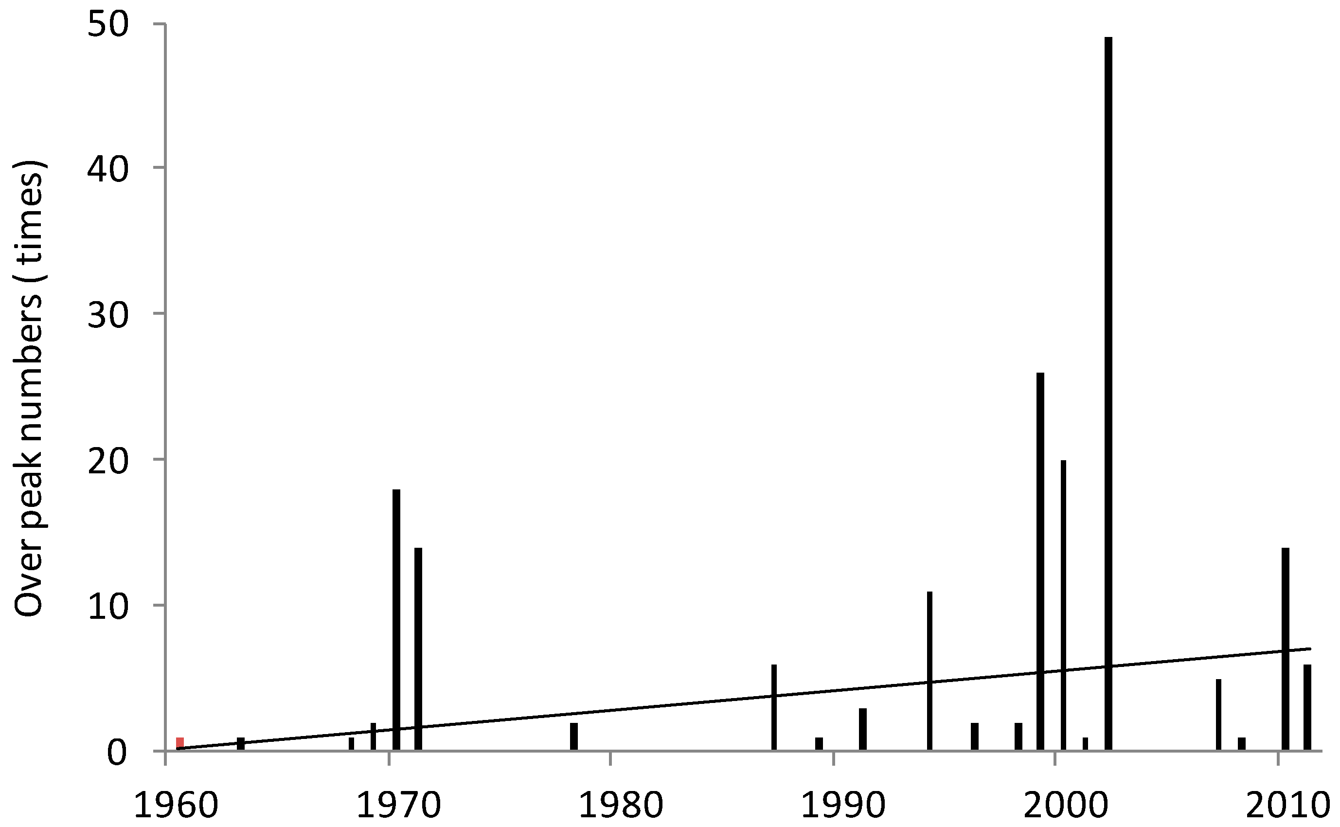
Figure 4.
Results for change point detection for AM-SPRT series at the KSWT station.

Figure 5.
Empirical and theoretical return levels of AM series in five hydrological stations: (a) KSWT; (b) BY (c) DSK; (d) HSG; and (e) KRGT.
Figure 5.
Empirical and theoretical return levels of AM series in five hydrological stations: (a) KSWT; (b) BY (c) DSK; (d) HSG; and (e) KRGT.


Figure 6.
Empirical and theoretical return levels of POT series in five hydrological stations: (a) KSWT; (b) BY; (c) DSK; (d) HSG; and (e) KRGT.
Figure 6.
Empirical and theoretical return levels of POT series in five hydrological stations: (a) KSWT; (b) BY; (c) DSK; (d) HSG; and (e) KRGT.

Figure 7.
Comparation of the GEV and GDP estimated flood discharges for a 100-year return period.

Figure 8.
Annual mean precipitation and temperature changes at four typical watersheds in middle Tianshan Mountains: (a) Kaidu watershed; (b) Manas watershed; and (c) Huangshui and Qingshui watershed.
Figure 8.
Annual mean precipitation and temperature changes at four typical watersheds in middle Tianshan Mountains: (a) Kaidu watershed; (b) Manas watershed; and (c) Huangshui and Qingshui watershed.

Figure 9.
Changes on magnitude and frequency of the extreme rainfall events in typical watersheds of middle Tianshan Mountains: (a) Kaidu; (b) Manas; and (c) Huangshui and Qingshui.
Figure 9.
Changes on magnitude and frequency of the extreme rainfall events in typical watersheds of middle Tianshan Mountains: (a) Kaidu; (b) Manas; and (c) Huangshui and Qingshui.

Figure 10.
Variations of: (a) over peak numbers and (b) volume contributions) for summer extreme flow and precipitation in the Kaidu watershed.
Figure 10.
Variations of: (a) over peak numbers and (b) volume contributions) for summer extreme flow and precipitation in the Kaidu watershed.

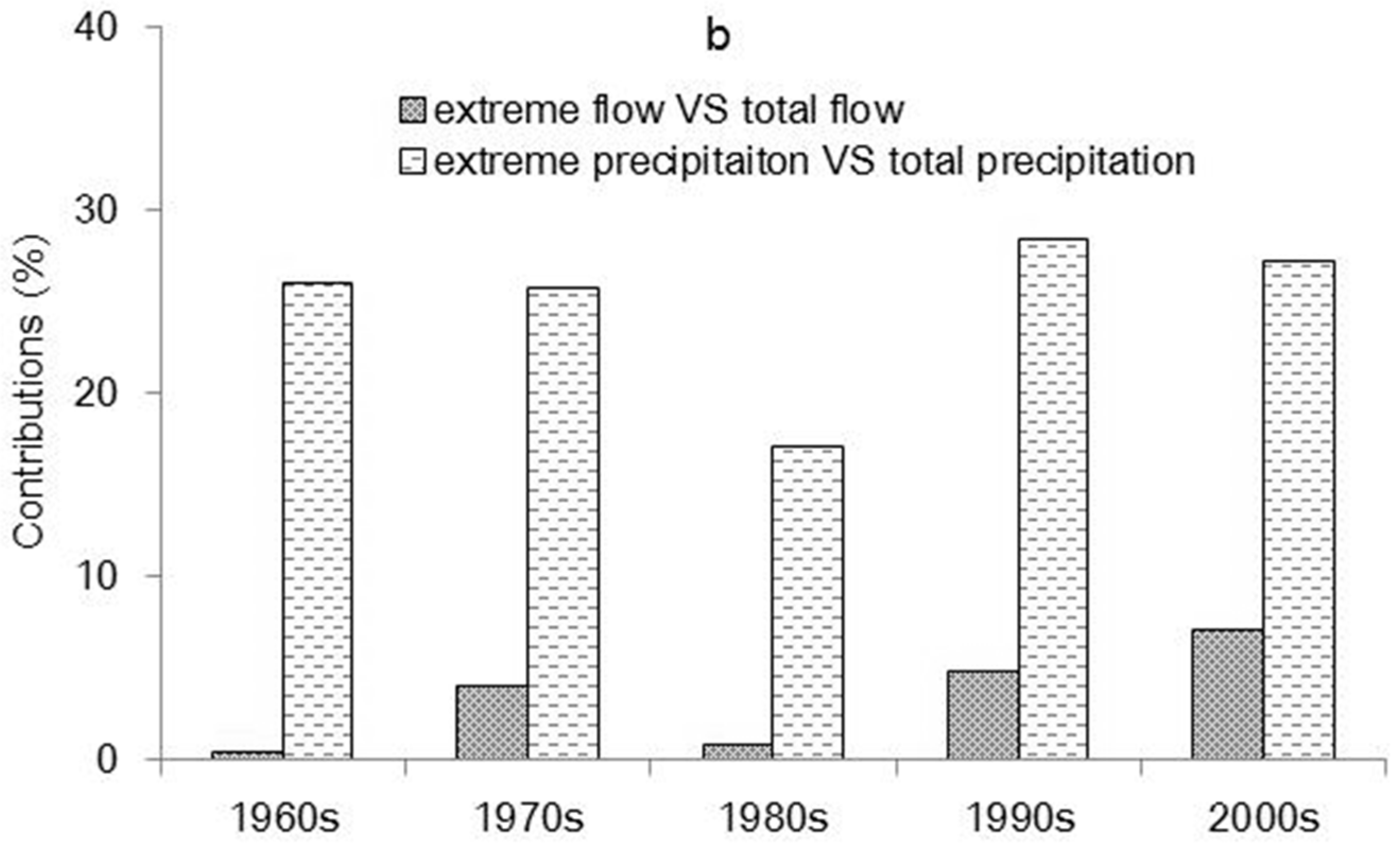
Figure 11.
Comparison of the climate indices which related to spring extreme flow in KD and HS: (a) precipitation in winter; (b) maximum snow depth; (c) mean temperature in winter; and (d) active accumulated temperature in spring.
Figure 11.
Comparison of the climate indices which related to spring extreme flow in KD and HS: (a) precipitation in winter; (b) maximum snow depth; (c) mean temperature in winter; and (d) active accumulated temperature in spring.


Table 1.
Information of hydrological stations.
| Stations | Drainage Area (km2) | Time Interval | Longitude | Latitude | |
|---|---|---|---|---|---|
| Manasi River | KSWT | 5167.44 | 1958–2011 | E84.93 | N43.07 |
| Kaidu River | BY | 6645.60 | 1978–2011 | E84.08 | N42.55 |
| DSK | 18653.79 | 1958–2011 | E82.95 | N42.19 | |
| Huangshui River | HSG | 4299.53 | 1958–1989 | E85.79 | N42.44 |
| Qingshui River | KRGT | 1047.66 | 1958–1989 | E86.55 | N42.36 |
Table 2.
Results of change point detection for eight extreme flow indicators.
| Rivers/Stations | AM | AMT | POT | POTN | |||||||||
| p Value | Change Point | Sig. | p Value | Change Point | Sig. | p Value | Change Point | Sig. Level | p Value | Change Point | Sig. | ||
| Manasi River | KSWT | 0.100 | R | 0.898 | R | 0.047 | 1986 | * | 0.149 | R | |||
| Kaidu River | BY | 0.455 | R | 0.971 | R | 0.488 | R | 0.187 | R | ||||
| DSK | 0.113 | R | 0.470 | R | 0.499 | R | 0.155 | R | |||||
| Huangshui River | HSG | 1.000 | R | 0.282 | R | 0.318 | R | 1.000 | R | ||||
| Qingshui River | KRGT | 0.298 | R | 0.948 | R | 0.059 | R | 0.622 | R | ||||
| AM-SPR | AM-SPRT | AM-SUM | AM-SUMT | ||||||||||
| p Value | Change Point | Sig. | p Value | Change Point | Sig. | p Value | Change Point | Sig. | p Value | Change Point | Sig. | ||
| Manasi River | KSWT | 0.959 | R | 0.004 | 1978 | ** | 0.100 | R | 0.897 | R | |||
| Kaidu River | BY | 0.620 | R | 0.595 | R | 0.282 | R | 0.541 | R | ||||
| DSK | 0.338 | R | 0.441 | R | 0.123 | R | 0.075 | R | |||||
| Huangshui River | HSG | 0.461 | R | 0.511 | R | 0.130 | R | 0.282 | R | ||||
| Qingshui River | KRGT | 0.865 | R | 0.949 | R | 0.228 | R | 0.969 | R | ||||
* indicate the change point is exist at a significance level of 0.05; ** indicate the change point is exist at a significance level of 0.01.
Table 3.
Parameter estimation and accuracy evaluation under the GEV and GDP distributions for AM and POT series.
Table 3.
Parameter estimation and accuracy evaluation under the GEV and GDP distributions for AM and POT series.
| Rivers | Stations | Time Series | Parameters | Best Fit PDF | K-S Test | Correlation | ||
|---|---|---|---|---|---|---|---|---|
| Manasi River | KSWT | AM | 231 | 66.43 | 0.29 | Frѐchet | 0.109 | 0.994 |
| POT | 226 | 52.39 | 0.23 | Pareto | 0.207 | 0.997 | ||
| Kaidu River | BY | AM | 73.9 | 46.95 | 0 | Gumbel | 0.258 | 0.885 |
| POT | 110 | 32.75 | 0 | Exponential | 0.336 | 0.989 | ||
| DSK | AM | 353 | 92.49 | 0.26 | Frѐchet | 0.148 | 0.991 | |
| POT | 404 | 61.54 | 0.15 | Pareto | 0.223 | 0.998 | ||
| Huangshui River | HSG | AM | 70.1 | 62.74 | 0 | Gumbel | 0.197 | 0.993 |
| POT | 86.3 | 25.80 | 0.30 | Pareto | 0.104 | 0.988 | ||
| Qingshui River | KRGT | AM | 46.2 | 23.88 | 0.52 | Gumbel | 0.196 | 0.986 |
| POT | 28.1 | 14.44 | 0.51 | Pareto | 0.211 | 0.990 | ||
Table 4.
Comparison of observed and GEV model predicted annual maximum discharge for return period of 5year, 10 year, 20 year, and the longest records.
Table 4.
Comparison of observed and GEV model predicted annual maximum discharge for return period of 5year, 10 year, 20 year, and the longest records.
| Stations | Number of Years | Observed | GEV Prediction | Error (%) | |
|---|---|---|---|---|---|
| 5 year | KSWT | - | 330 | 360 | 9.1 |
| BY | - | 137 | 136 | −0.7 | |
| DSK | - | 478 | 488 | 2.1 | |
| HSG | - | 170 | 169 | −0.5 | |
| QSH | - | 85 | 90 | 5.9 | |
| 10 year | KSWT | - | 355 | 428 | 20.6 |
| BY | - | 194 | 186 | −4.1 | |
| DSK | - | 621 | 623 | 0.3 | |
| HSG | - | 230 | 212 | −7.8 | |
| QSH | - | 141 | 150 | 6.4 | |
| 20 year | KSWT | - | 430 | 511 | 18.8 |
| BY | - | 243 | 270 | 11.1 | |
| DSK | - | 652 | 735 | 12.7 | |
| HSG | - | 238 | 241 | 1.3 | |
| QSH | - | 162 | 206 | 27.2 | |
| longest record | KSWT | 54 | 789 | 721 | −8.6 |
| BY | 33 | 253 | 286 | 13.0 | |
| DSK | 54 | 793 | 940 | 18.5 | |
| HSG | 31 | 244 | 280 | 14.8 | |
| QSH | 31 | 199 | 235 | 18.1 |
Table 5.
Comparison of observed and GDP model predicted over peak discharge for return period of 5 year, 10 year, 20 year, and the longest records.
Table 5.
Comparison of observed and GDP model predicted over peak discharge for return period of 5 year, 10 year, 20 year, and the longest records.
| Stations | Number of Events | Observed | GDP Prediction | Error (%) | |
|---|---|---|---|---|---|
| 5 year | KSWT | - | 421 | 423 | 0.5 |
| BY | - | 197 | 196 | −0.5 | |
| DSK | - | 597 | 600 | 0.5 | |
| HSG | - | 171 | 172 | 0.6 | |
| QSH | - | 139 | 138 | −0.7 | |
| 10 year | KSWT | - | 495 | 496 | 0.2 |
| BY | - | 222 | 221 | −0.4 | |
| DSK | - | 644 | 662 | 2.8 | |
| HSG | - | 230 | 220 | −4.3 | |
| QSH | - | 148 | 161 | 8.8 | |
| 20 year | KSWT | - | 750 | 600 | −14.0 |
| BY | - | 244 | 240 | −1.6 | |
| DSK | - | 702 | 796 | 13.4 | |
| HSG | - | 239 | 265 | 10.9 | |
| QSH | - | 165 | 198 | 20.0 | |
| longest records | KSWT | 172 | 789 | 720 | −8.7 |
| BY | 129 | 253 | 273 | 7.9 | |
| DSK | 176 | 793 | 830 | 4.7 | |
| HSG | 92 | 354 | 338 | −4.5 | |
| QSH | 96 | 199 | 246 | 23.6 |
© 2018 by the authors. Licensee MDPI, Basel, Switzerland. This article is an open access article distributed under the terms and conditions of the Creative Commons Attribution (CC BY) license (http://creativecommons.org/licenses/by/4.0/).
Share and Cite
MDPI and ACS Style
Ma, Y.; Huang, Y.; Liu, T. Change and Climatic Linkage for Extreme Flows in Typical Catchments of Middle Tianshan Mountain, Northwest China. Water 2018, 10, 1061. https://doi.org/10.3390/w10081061
AMA Style
Ma Y, Huang Y, Liu T. Change and Climatic Linkage for Extreme Flows in Typical Catchments of Middle Tianshan Mountain, Northwest China. Water. 2018; 10(8):1061. https://doi.org/10.3390/w10081061
Chicago/Turabian StyleMa, Yonggang, Yue Huang, and Tie Liu. 2018. "Change and Climatic Linkage for Extreme Flows in Typical Catchments of Middle Tianshan Mountain, Northwest China" Water 10, no. 8: 1061. https://doi.org/10.3390/w10081061
Note that from the first issue of 2016, this journal uses article numbers instead of page numbers. See further details here.