Detection of Sediment Trends Using Wavelet Transforms in the Upper Indus River


College of Earth & Environmental Sciences, University of the Punjab, Lahore 54590, Pakistan
*
Authors to whom correspondence should be addressed.
Water 2018, 10(7), 918; https://doi.org/10.3390/w10070918
Submission received: 24 May 2018
/
Revised: 28 June 2018
/
Accepted: 30 June 2018
/
Published: 11 July 2018
(This article belongs to the Special Issue Watershed Hydrology, Erosion and Sediment Transport Processes
)
Abstract
:Sediment load trends play a key role in modelling either river morphology or reservoir sedimentation. In this study, suspended sediment concentration (SSC) series of four representative gauging stations of the Upper Indus Basin (Yugo, Dainyor, Bunji and Besham Qila) were selected and updated from a vast network of hydro-meteorological stations being operated and maintained by Water and Power Development Authority (WAPDA) of Pakistan from the 1960s up to now. The temporal variations in the series were analysed using the wavelet transform (WT) method. The WT method disclosed the temporal and frequency information for trend estimation analysis by decomposing data on several levels. The results of the combined methods, WT and Mann–Kendall (MK) trend tests, revealed that the annual sediment time series, available since the 1960s for some stations, exhibited a statistically insignificant trend due to statistically significant intra-annual (monthly) shifts. Generally increasing trends in the winter months and decreasing trends in summer months for major sub-catchments of Upper Indus Basin (UIB) were detected. However, the study also proved that the identified intra-annual or monthly shifts in upper sub-catchments were being neutralized as the sediment progressed downstream. This study of variations in sediment trends was required for constructing sediment budgets and sustainable operations of existing and planned future water storage along the tributaries and the main stem of the Upper Indus River.
1. Introduction
A gradually growing body of evidence and research was present and proved that, since the start of the current century, the water availability in the Upper Indus Basin (UIB) had been changing from summer months to the non-summer months due to a shift in meteorological variables [1,2]. This shift most probably has also been liable to bring changes in erosion and deposition patterns in the catchment. Due to the heavy suspended sediment concentration (SSC) supply from the geologically newer Hindukush–Karakoram–Himalaya (HKH) ranges, the reservoirs in UIB were filling up with sediment deposits. This deposition was rapidly decreasing the storage capacities and putting more burden on the existing water supply systems in the form of excessive ground water extraction, which was already up to 40% (10% more than international recommendations). On the other hand, to meet the needs of the growing population, the country needed more water storage facilities for irrigation, power generation and drinking. The present storage facilities could store only 10% of the available rivers’ flow. However, the construction of new storage facilities required huge financial investment and advanced sediment management practices. For example, an only 10 m raising of the Mangla Dam—the second largest dam in Pakistan—cost one billion USD and 45,000 people were displaced. However, this huge investment only recovered and increased its storage from 7.1 billion m3 (original) to 9.1 billion m3. Similarly, another dam, the Warsak dam, lost all of its live storage capacity of 167 million m3 just in 30 years due to 60 Mt sediment supply from its catchment [3]. No post-construction technical and non-technical measures could reverse the process. Keeping in mind the importance of sustainable reservoir capacities and hydro-morphodynamic modelling, it is necessary to study the sediment trends for the Indus River. These trends could provide support for better sediment management practices (such as sediment supply, sediment routing or sediment removal) for existing, planned hydraulic structures and construction of sediment budgets in the study area.
Different approaches, techniques and statistical methods have been advanced and practised by researchers to study riverine dynamics. To detect trends in hydro-met data, a number of techniques have been developed by researchers. The most often used include: evaluating discharge–total suspended solids (Q–TSS)/SSC and time–discharge (T–Q) relationships over progressive periods by parametric regression procedures as comprehensively elaborated by [4], two-sample t-test and estimates of change magnitude based on the difference in sample means [5], and important parametric tests like MK [6,7], Rank Sum test [8], Pettitt test [9], Serial correlation test, etc. A very vital study was conducted by [10] establishing a framework and basis for selection and application of methods for trends. Many regional studies of capturing trends in hydro-met variables have been conducted to date, following the standard procedures/analytical techniques referred above. Much work on trends has been done for the high sediment laden Yellow River in China. A recent study in this respect was done by [11]. Sediment Budgeting of large basins is another robust, data intensive and difficult approach to study the dynamics of sediment in the selected area. Ref. [12] prepared an initial framework for collection, processing and collation of sediment data in a good effort to formulate a sediment budget of UIB.
In assessing spatial and temporal dynamics in sedimentological and hydrological variables, it was assessed that non-parametric tests were more powerful as compared to their parametric counterparts, due to the fact that sedimentological variables were not normally distributed and because of the highly nonlinear nature of sediment transport processes. Therefore, we applied the Mann–Kendall (MK) test that had been widely used in environmental studies [13,14] due to its simplicity, robustness, and ability to handle the outliers in the data samples. Since the development of the method, it had been modified several times, such as inclusion of the seasonal Kendall (SK) test to handle seasonality in the data, or modifying it in an attempt to remove or lessen serial/auto correlation in the data. Therefore, it had been well proved by different researchers that the MK Test was not appropriate for applicability in detecting auto/serial correlation, and depended more on data size and magnitude of the trends. Therefore, it seemed rational to couple an MK Test with a method that could deal with trends in sedimentological and hydrological variables at different temporal resolutions for different regions.
To eliminate the effects of auto/serial correlation, Discrete Wavelet Transforms (DWT) have been successfully used to split the given signal/sample in temporal and frequency domains and to extract the information at different resolutions. Ref. [13] provides a list where the DWT has successfully been used in environmental studies. For example, Ref. [14] determined the hydrological trends in the Marmara region of Turkey by using the detailed and approximate coefficients of wavelet at different resolutions in the MK Test. Moreover, Ref. [15] also used a Wavelet Trend Test to analyse temporal changes in the hydrological and sedimentological series of the Pearl River in China. Based on the above cited research, we used the wavelet trend test, in this study, at different resolutions to detect the temporal and spatial trends in hydrological and sedimentological parameters. In addition, we also combined different detail coefficients (D) of these parameters extracted at different resolutions along with approximation coefficient (A) in the MK test.
Contrary to trends in water availability, not much had been done to quantify the SSC trends due to the highly nonlinear nature of the process for the upper Indus River. The nonlinearity included in the high frequency components (i.e., annual and inter-annual time scales) of a time series could affect the identification of trends in the series [14]. In the current research study, to eliminate the impacts of high frequency components on the identification of trends, the wavelet transform method was utilized. For purposes of decomposition and rebuilding a time series at different scales, the wavelet transform method was a powerful tool for multi-scale detection. By low-pass sieving of the original data, the low frequency components were collected via a rebuilding of the low frequency coefficients. The trend of the time series at required time scales could be represented by the change in trend of the low frequency components. In the current study, the Daubechies 1 (Db1) wavelet, having a similar shape structure to the hydrological series, was used to break and rebuild the annual hydrological series by following Mallat’s algorithm. The Mann–Kendall (MK) trend test, was applied to identify the trend changes in the hydrological series based on the low frequency components, as it was widely used in the identification of trend changes in hydro-meteorological data series. Therefore, for discovering monotonic/unvarying trends, the MK trend test was an established non-parametric method in vogue. The null hypothesis, , was that a sample of data, , was independent and identically distributed with no trend. The null hypothesis, , was acceptable if , where Z and P were the significance levels of the tested and computed standardized statistics, respectively [16]. In the current study, p = 0.05 was applied as the significance level.
The investigations carried out in the present study were envisioned to have vital impacts on the quality and employed methodologies of future sediment research in the region with long-term effects on the existing/planned reservoirs in the study area. The overall objective of the research was: (1) detailed investigations into the revealing/non-revealing, identification and quantification of trends, across the spatial distribution of selected Main UIB and important sub-catchments, by utilizing the DWT method coupled with an MK test; (2) Identification of inter and intra annual trends of selected Main Indus and major sub-catchments; (3) Enabling designers of future dams/reservoirs in the region to consider and incorporate the findings in the present research, for effective and efficient designs; and (4) Identification of an analytical method for sedimentation studies of UIB and for other riverine regions of the world.
2. Study Area and Data
The study area was comprised of the Upper Indus basin (UIB). The Indus River was one of the longest and most significant rivers of the world as it fed the world’s largest contiguous irrigation system. In 1999–2000, the total irrigated area in Pakistan was 181,000 Km2 [17,18]. The waters of the Indus and its tributaries were also essential for power generation, as hydropower contributed about 29 percent to the National Power Grid of Pakistan [18].
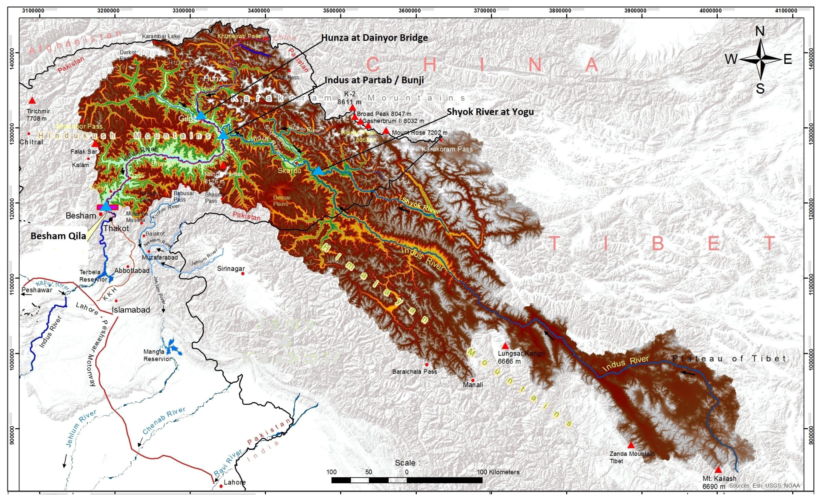
Originating from the frozen deserted Tibetan Plateau and passing through whole Pakistan, while gathering flows and sediment from its large tributary of Shyok River, it enters the Baltistan Area of Pakistan. Shigar River, another large tributary of the Indus, draining the Karakorum range and adjacent areas, joined the mother river near the Town of Skardu. Skardu valley is a large wide valley constricted into a narrow gorge downstream of Kachura. This gorge contained in its valley the Indus flows with steep gradients between one of the tallest peaks amassing their drainage and confluencing with the Gilgit River just upstream of the town of Bunji. Hunza River, a sediment laden river (the analysis of which was included in this study) entered the Gilgit River some kilometers above the Gilgit–Indus joint. Another significant tributary, namely the Astore River, entered the main Indus a few kilometers downstream of Bunji (Figure 1). The Astore River drained the eastern face of the Nanga Parbat Massif. Many small and large tributaries after Indus–Astore confluence entered the main river up to Besham Qila and further up to Tarbela (the southernmost boundary of UIB) from the left and the right banks. To name a few, from the left side, such as: Gunar Gah, Butto Gah, Thor Gah, Spat Gah, Chor Nullah, Allai Khwar, Siran River, etc. In addition, the major right bank tributaries entering the main stem of Indus were: Darel and Tangir Rivers, Kandia River, Keyal Khwar, Duber Khwar, Gorband and Brandu Rivers. The sediment entry coming from the catchment area downstream of Bunji up to Tarbela was significantly less, as compared to the sediment contribution from upstream of Bunji [19].
The climate of the UIB was predominately arid to semi-arid in the north with precipitation ranging annually between 80–180 mm due to the massive rain shadow being cast by the Nanga Partab Massif. Rain in the northern part was from winter westerly currents/disturbances. However, occasionally very strong monsoon currents did manage to cross that barrier and dropped rains as far as Gilgit and Skardu Towns. Moving downward in the southerly direction along the Indus, the rain shadow was broken after crossing the town of Dasu. Moderate to heavy and progressively increasing summer monsoon spells occurred between Dasu and Besham Qila/Tarbela, ranging annually between 1000–1500 mm. The Upper Indus Basin as demarcated was shown in Figure 1. The normal precipitation map of Pakistan, including UIB, with four selected stations marked is shown in Figure 2.
In the present research, the hydrological data consisted of the intermittent suspended sediment concentration (SSC) samples at four (4) gauging stations, namely Yugo, Dainyor, Bunji and Besham Qila, on the main Indus River and tributaries from the 1960s/1970s to date (Table 1, Figure 3). These selected gauging stations included important and representative measuring points in the vast UIB Gauging Network. The station at Yugo on River Shyok has been operational since 1973 up to now. Flows and sediment from the Tibetan Plains and the Leh region were drained to this point. The station at Dainyor on the Hunza River has been operational since 1966 up to now. The station recorded the heaviest sediment concentrations in all of the UIB and therefore had critical importance in sediment research in the region. Many landslides damming up the valleys of Hunza sub-basin had occurred in the past and continued to happen to this day. The Station at Partab/Bunji has been operational since 1960 on the main Indus. Data from Bunji was available up to 2009 as the gauging cableway was swept away in the Catastrophic Flood of 2010. The station recorded data on the Main Indus after confluence of a number of sediment carrying tributaries and as such its analysis was very important. The last station that had been analyzed in the present study was Besham Qila on the main Indus in the Monsoon region of UIB. It has been operational since 1969 up to now. Besham Qila was the last measuring point before the Indus entered the huge Tarbela Reservoir. The data originating from Besham Qila formed the basis of sediment studies for the reservoir and was of vital importance with regard to any present/future sediment strategies. This hydromet data, along-with the vast gauging network in the UIB and the Lower Indus Basin (LIB) was collected by the Surface Water Hydrology Project (SWHP) of Water and Power Development Authority (WAPDA), using current meters for discharges and U.S. Geological Survey (USGS) standard samplers for SSCs. The data for non-observed days of SSCs were estimated using sediment rating curves developed by WAPDA or consultants). The quality of the hydro-meteorological data was under strict control and standard scrutiny of the relevant organizations before publishing in the form of annual booklets. More information about data collection, handling, and data quality was available in [20].
3. Methods
Changes in the sediment concentrations of the Upper Indus Basin (UIB), especially for the glacier melt dominated zone (Dainyor, Yugo and Partab Bridge), were analyzed for the whole UIB (up to Besham Qila), which was further impacted by summer rainfall in the monsoon season. In order to conduct analysis, the suspended sediment concentration (SSC) samples were first decomposed into time and frequency domains. The decomposition alone and with non-parameter trend estimation methods (i.e., Mann–Kendall test) was used to find out periodicities responsible for trends in SSC.
3.1. Wavelet Transform
Recently, wavelet analysis has earned a wide acceptance in a wide range of science and engineering. Some of the latest studies utilizing the wavelet analysis are [13,14,15,19,21]. The technique has also been used in: data and image compression; partial differential equation solving; transient detection, pattern recognition, texture analysis, noise reduction, trend detection, etc. Wavelets are found to be more effective tools than the Fourier transform (FT) in analysing the non-stationary time series. Instead of FT, which analyses the data in two dimensions, i.e., time and frequency, wavelet outputs’ three dimensions, i.e., time, space and frequency. This provides an opportunity to examine the variation in the hydrological processes.
Discrete Wavelet Analysis
Wavelet transform (WT) breaks data series into logically ordered wave-like oscillations (wavelets) analogous to data vis-à-vis time within a range of frequencies. The original time series can be depicted with regard to a wavelet expansion that uses the coefficients of the wavelet functions. Several wavelets can be made from a function known as a “mother wavelet”, which is restricted in a finite/bound interval. That is, WT expresses/breaks a given signal into frequency bands, and then analyses them in time. WT is widely categorized into Continuous Wavelet Transform (CWT) and Discrete Wavelet Transform (DWT). CWT is defined as the sum over the whole time of the signal to be analysed, multiplied by the scaled and shifted versions of the transforming function . The CWT of a signal is expressed as follows:
where ‘*’ denotes the complex conjugate. CWT looks for correlations/mutual relationships between the signal and wavelet function. This measurement is done at distinct scales of a and locally around the time of b. The result is a ripple/wavelet coefficient outline sketch. However, enumerating the wavelet/ripple coefficients at every likely scale (resolution level) demands a huge amount of data and calculation time. DWT analyses a given time series with distinct resolutions for a distinct range of frequencies. This is done by decaying the data into coarse approximation and detail coefficients. For this, the scaling and wavelet/ripple functions are utilized. Choosing the scales a and the positions b based on the powers of two (binary scales and positions), DWT for a discontinuous time series , becomes:
where i is integer time steps and N = ); m and n are integers that control, respectively, the scale and time; is wavelet coefficient for the scale factor and the time factor . The original signal can be built back/recreated using the inverse discrete wavelet transform as follows:
or in a simple form as:
where is called an approximation sub-signal at level M and are details sub-signals at levels . The approximation coefficient represents the high scale low frequency component of the signal, while the detailed coefficients represent the low scale high frequency component of the signal.
There are a number of mother wavelets such as: Haar; Daubechies; Coiflet and Biorthogonal. Normally, Daubechies, belonging to Haar wavelet, achieves improved results in sediment transport processes due to its inherent capacity to discover time localization information. In dealing with the annual recurrence and hysteresis/lag phenomenon, time localization information is beneficial in flow discharge and sediment processes. The Coiflet wavelet is more symmetrical than the Daubechies wavelet. Likewise, Biorthogonal wavelets have the characteristic of linear phase, which is required for signal rebuilding [21]. The appropriateness and selection of mother wavelet is dependent on application type and characteristics of data.
3.2. Trend Estimation
Mann–Kendall Test (MK)
The MK test is an non-parameter test that has been extensively applied to check consistency against trends in hydrology and sediments [19]. The Mann–Kendall (MK—[6,7]) test has the ability to identify the presence of trends in time series without the effect of data that stands out, i.e., outliers. By the application of normal approximation, the MK test statistic S is calculated as follows:
where and are the adjoining data values, S is the sum of positive or negative signs, n is the number of data values and
The MK test has two important parameters, i.e., level of significance and slope. The former indicating strength and the latter one indicating trend magnitude and direction. In case of a number of tied-up or similar data values, a specified method for values greater than 40 is used ([7], as reported by [22]). The S’s oscillation in (Equation (7)) caters to these ties, where q is the number of tied groups and is the number of data in the p group:
An MK statistic Z is computed using Equation (8), after determining S and its variance. The positive value for Z indicating up-sloping trend and negative value indicating a down-sloping trend. In case of no identifiable trend, the MK statistic Z has a standard normal distribution:
A somewhat changed version of the MK test to identify the season-wise monotonic or recurring trends—namely seasonal Kendall (SK)—is sometimes employed, which runs the original MK test on each season/recurrent period (k) separately, where k can refer to any period of time within a year (e.g., months or four quarters of a year). Each SK statistic () for m number of seasons is added, in order to determine the overall S statistic and the statistical significance of the trend is evaluated making use of the outcome of Equations (10) and (11) in Equation (8):
and
Ref. [23] showed that a positive serial correlation increased the deviation of the distribution of S , based on Monte Carlo sets of simulations, and thus increasing likelihood of dismissing the null hypothesis of no trend; similar findings were reported by [24]. Conversely, negative serial correlation reduced the variance/deviation of distribution and resulted in the underrating of significant trend detection likelihood. A correction factor to restrict the power of serial correlation was applied as described by [25] in Equation (8) as follows:
As a normal case, the sample serial correlation coefficient replaces the population serial correlation coefficient :
The MK statistics is expanded or shrunken, by the correction factor if positive or negative serial correlation is found.
Sen’s slope estimator [26] is an estimate of trend extent, closely related to the MK test procedure. Firstly, the slope estimates of pairs of data of the k-season, are determined by:
for all and . The median of these values is Sen’s slope estimator :
4. Results and Discussion
4.1. Inter-Annual Trends
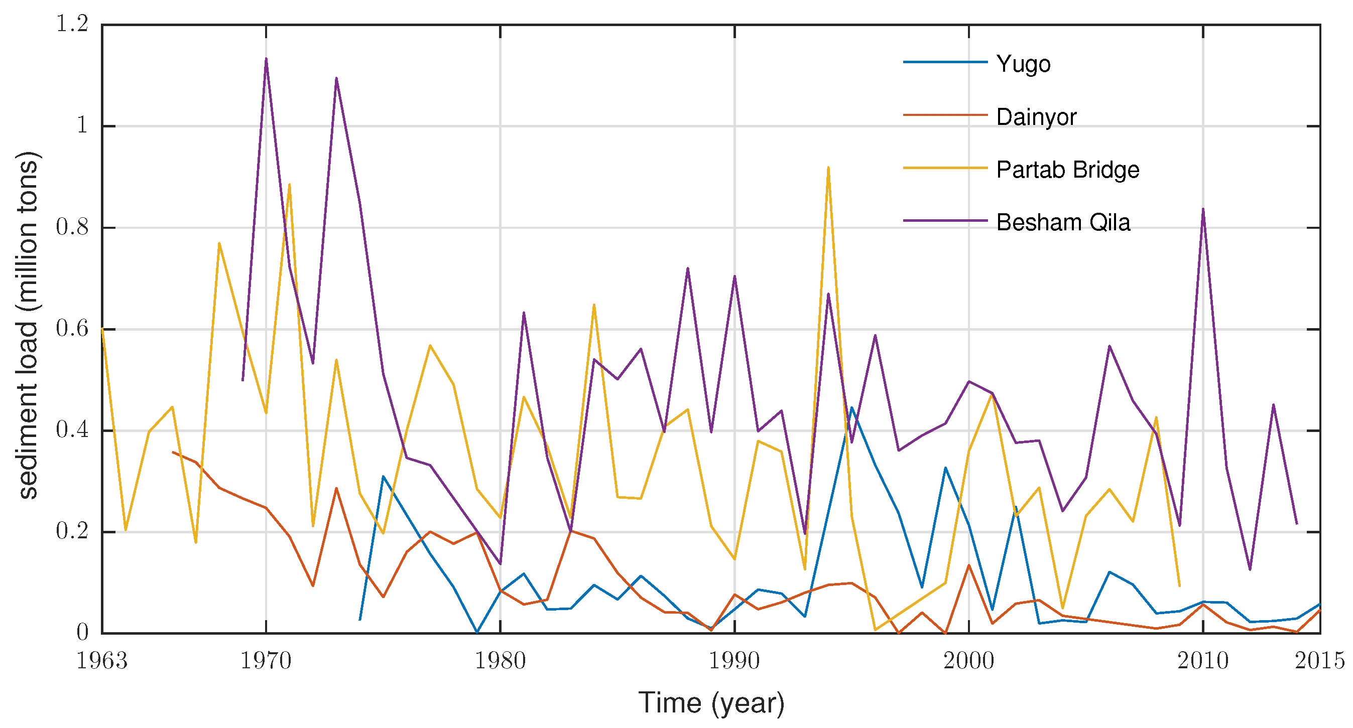
Inter-annual trends were analyzed using mean annual data in decomposition and the Mann–Kendall trend test estimation process. The frequency of high and low annual suspended sediment concentration (SSC) at Dainyor gauge stations located in west Karakoram catchments has been increasing (Figure 4). However, the frequency of high and low annual SSCs at the Yugo gauge station located in the east Karakoram catchment has been decreasing (Figure 5). At the confluence of both catchments’ outlet at the Partab Bridge gauge station, the frequency of high and low annual SSC has been slightly increasing (Figure 6). Similarly, downstream of the whole upper Indus catchment at Besham Qila (additionally influenced by rainfall) again has a slightly increasing trend in SSC (Figure 7). The SSC trends at Dainyor might be related to the trends in discharge, where the discharge in western Karakoram has been increasing with a rate of m3/s since 1995 [2]. Similarly, there was also an annual decreasing trend with a magnitude of m3/s in discharge at the Yugo gauge station [2]. The decreasing trend was also related to a slight decrease in annual concentration at the same gauge station (Figure 5). The similarity in discharges and SSCs was also found at Partab Bridge and Besham Qila. The main reason for increasing annual discharges at Dainyor, Partab Bridge, and Besham Qila related to a change in temperature in high flow contributing months. The change in flow of these months also caused a change in erosion and deposition processes in the catchments. On the other hand, the annual decrease in both discharges and SSC at the Yugo gauge station may be ascribed to summer cooling together with certain changes in prevailing precipitation regimes. Similarly, the changes in annual trends have also been driven by predominant intra-annual trends.
The Discrete Wavelet Transformation (DWT) method inherently takes care of auto/serial correlation, if present, in the original series and eliminates effects of seasonality and discharge on the SSCs. The transformed/corrected SSC data is then fed into the MK test to check for trends. In this way, the chances of auto correlation and discharge influencing the SSCs are minimized. As pointed out by [10] in the last sentence of his conclusion that: “...particular issues that need additional development are methods that make possible use of existing data (in light of potentially strong serial correlation in the data)...”, the indicated method of DWT coupled with an MK test indeed has such a capability.
4.2. Intra-Annual Trends
In contrast to annual trends, the suspended sediment concentration (SSC) at the Dainyor gauge station have been increasing in pre and post summer months (Table 2). However, the SSC has been significantly decreasing (p-value < 0.05) in summer months. At the Yugo gauge station, the intra-annual trends, similar to inter-annual trends, have shown a decreasing trend. The Partab Bridge gauge station has shown an increasing trend except May (Table 2). The most surprising situation is at Besham Qila, where SSC from January to March has been increasing, while, from April to December, it has been decreasing.
The significant increasing trend in pre and post summer months at Dainyor gauge station (representing western Karakoram suspended sediment concentration (SSC)) might have been caused by a significant increase in the run-off in these months. The increased run-off/river flow might have been either causing erosion in the catchment or eroding temporary sediment storage in the river channel that is deposited during summer months. On the other hand, the decrease in SSC during summer was due to a decrease in sediment load carrying capacity of the river, which deposited additional eroded sediments in the main river channel. The selected stations, except Besham Qila, lie in an arid to semi-arid region of UIB where a rain shadow is cast by the high Nanga Parbat Massif. The average rainfall depth is between 150–200 mm annually. The discharge and the sediment regime of UIB are predominated by the snow and glacial melt waters in summers and reduce considerably during winters. Rainfall contribution to discharge is non-significant at stations of Yugo, Dainyor and Partab, whereas some contribution of monsoonal rainfall occurs at Besham in the lower portions of UIB. No reservoirs, diversion structures or significant anthropogenic activity (industries, agriculture, etc.) exist up to now to alter the natural regime of sediments and the detected trends, as such, are the result of natural activity. The Sediment–Discharge (S–D) relationships of the selected stations exhibit a very good long-term relation with R2 values above 0.9. However, the study of positive/negative hysteresis phenomenon as done by [28] was considered to be outside the purview of the present study, as only the annual/monthly SSCs were accounted for and their trending causes or their relationships with discharge were not considered.
Similarly, the only significant decreasing trend in SSC during summer at east Karakoram have been caused by a cooling effect, which has been causing a decrease in overall discharge in the summer [29]. This trend is called Karakoram Anomaly. The effect of a trend noticed at both gauge stations representing eastern and western Karakoram have been cancelled at a downstream gauge station, i.e., Partab Bridge. Except for significant trends in January and February, which have also been caused by substantial temporary storage (in summer), there is no significant trend (Table 2). Substantial sediment storage in the Partab Bridge–Besham Qila Reach [30] has been causing significant decreasing trends during summer at Besham Qila. However, the catchment area represented by Besham Qila is also influenced by monsoon rainfall, and its minor (10–30%) contribution is not sufficient to transport enormous incoming sediment further downstream. Surprisingly, the trends in flow discharges at these gauge stations are different than trends in SSCs. For example, the discharge trends in summer (July–September) have statistically been significantly increasing [2]; however, SSC in summer is either showing a decreasing trend or no trend (Table 2).
The suspended sediment transport process is different than water flow due to different grain sizes, densities, shear stresses, sediment concentrations, bed roughness, and effective discharges, etc. The effective discharge is the class of flow where the majority of sediment load is transported. Although there are no land use changes and hydraulic structures in the UIB, due to the complex nature of the sediment transport process, the trends in discharges at different gauge stations can’t be used in a simple way (without considering trends for sediment loads.
As the Himalayas are geologically younger compared to other mountain ranges, the sediment load of Indus is amongst the highest in the world. Landslides occur frequently in the selected catchments of the UIB, especially the Hunza catchment. A recent landslide occurred in April 2010, which has permanently dammed up the river at that point, may be one of the reasons for low SSCs in Hunza during summer months.
Another major landslide occurred in the Hunza valley in 1974. After construction of the Tarbela dam, reduced sediment inflows of about 200 Metric tons were supported by the hydrographic surveys of the Tarbela reservoir due to the changed flow pattern and lower sediment concentration during the period 1974–2000. This could be attributed to the blockade of the Hunza river on 12 April 1974, which resulted in formation of a debris rock dam and caused a backwater as long as 8 km in the Hunza river. The situation was adequately explained by Wang Wenging et al. in “A surge Advance of the BALT BARE Glacier Karakorum Mountains, Lanzhou Institute of Glaciology and Cryopedology, Academia Sinica (Para-5), as: “On 12 April 1974, a rarely heavy mud-rock flow bursted out from the Balt Bare Valley by the Shashikat Village, where the Karakoram Highway, Pakistan passes through. The mud-rock flow with tremendous force swept off a household and a pedestrian. With the maximum discharge of about 6300 m/s, it poured out 5 mil m or more of earth, debris and rock during several minutes after running out of the mouth of the valley. Then, the Hunza River was blocked and a debris-rock dam was formed, which caused a backwater as long as 8 km, flooded a big bridge of 120 m in length and a section of highway about 4 km, so the communication was forced to be held up.” To further investigate the complex set of causes behind the trends in the SSCs, some linkage between seismicity and SSCs was also looked into. Although the scope of current study did not include investigations into the complex, natural and anthropogenic causes behind the trends, an initial attempt was made to understand the physical process involved in the unexplained trends. The UIB is a seismically active zone with many low to high earthquakes occurrences in the past [31]. One such massive event took place in October 2005 in the Azad Kashmir area. While the damage to life and property were phenomenal, the natural systems in the UIB were also severely shocked. In the coming sediment high flow season in 2006, Indus at Partab experienced the highest sediment load ever. This extraordinary situation was incidentally monitored by WAPDA’s Diamer Basha Consultants (DBC) in 2006. This high event was also estimated by [32] as 390 Mt SSL. In addition, Ref. [33] advanced the idea that the sediment disturbances were not only the case for high seismically active regions but also for regions with a weak to moderate seismic activity regime, and could help explain regional patterns and trends in sediment yields.
Other causes may be: short-time sediment storage along the main river and deposition/degradation. The concentration of sediment near the river bed affects the river transport capacity. The high concentrations during the summer increase the deposition rate in the channel due to high water depths and low velocities, which also decrease the corresponding settling velocities. Similarly, in winter months, when most of the flow in the river is contributed from the base flow, the relatively low SSC near the bottom causes more erosion of the deposits from the previous summer. Therefore, due to the complex nature of sediment transport processes, intra-annual trends in SSC are different than discharges.
As per our knowledge, the current study has not been conducted before; therefore, the findings are required for the construction of sediment load budget and relevant river studies of UIB [34] . This paper represented an initial stage in research designed to identify the hydrological impacts of climate change on the erosion and deposition patterns for the selected catchments of the UIB. This research could also be utilized to improve and modify future sediment studies for planned multi-purpose reservoirs in the study area.
5. Conclusions
The study deals with the trend detection in suspended sediment loads using the Mann–Kendall test coupled with a wavelet transform at the upper Indus Basin (UIB). Except an increase in annual low and high frequencies at the Dainyor gauge station, the annual sediment load trends at UIB are balanced by shifts in intra-annual trends from summer to the winter caused by the Karakorum Anomaly. However, sediment storage in the channel was not in the scope of this study, the decreasing trends at a much more downstream gauge might have been caused by substantial sediment storage in the main channel of the Indus River. Therefore, the current findings can help with better understanding and development of the sediment load budget for the upper Indus River. The findings will be of significant importance for future sedimentation studies of planned multi-purpose reservoirs for hydropower and irrigation in the study area and also has important implications/applications for the river environmental studies.
Author Contributions
Z.R.T. defined the problem, drew up the research plan, conducted research, and interpreted and drafted the outcome. S.R.A. calculated and analyzed sediment concentrations/data and helped review WT code and made significant contributions to improve it. I.A. supervised and directed the research study and critically reviewed the end result. Z.M. coordinated the collection of sediment data from data source authorities and carried out its analysis together with other authors. Also Z.M. substantially reviewed the article before and after submission.
Acknowledgments
The data for the study was provided by the Surface Water Hydrology Project (SWHP) of WAPDA. We appreciate their help and cooperation. This research did not receive any specific grants from funding agencies in the public, commercial, or not-for-profit sectors.
Conflicts of Interest
No conflict of interest is declared by the authors.
References
- Khan, F.; Pilz, J.; Amjad, M.; Wiberg, D.A. Climate variability and its impacts on water resources in the Upper Indus Basin under IPCC climate change scenarios. Int. J. Glob. Warm. 2015, 8, 46–69. [Google Scholar] [CrossRef]
- Hasson, S.; Böhner, J.; Lucarini, V. Prevailing climatic trends and runoff response from Hindukush– Karakoram–Himalaya, upper Indus Basin. Earth Syst. Dyn. 2017, 8, 337–355. [Google Scholar] [CrossRef]
- King, R.; Stevens, M. Sediment management at Warsak, Pakistan. Int. J. Hydropower Dams 2001, 8, 61–68. [Google Scholar]
- Montgomery, D.C.; Peck, E.A. Introduction to Linear Regression Analysis; John Wiley: New York, NY, USA; Brisbane, Australia, 1982. [Google Scholar]
- Lman, R.L.; Conover, W.J. A Modern Approach to Statistics; John Wiley: New York, NY, USA; Brisbane, Australia, 1983. [Google Scholar]
- Mann, H. Nonparametric tests against trend. Econmetrica 1945, 13, 245–259. [Google Scholar] [CrossRef]
- Kendall, M.G. Rank Correlation Methods, 4th ed.; Charles Griffin: London, UK, 1975. [Google Scholar]
- Bradley, J.V. Distribution-Free Statistical Tests; Prentice-Hall: Englewood Cliffs, NJ, USA, 1968. [Google Scholar]
- Pettitt, A.N. A non-parametric approach to the change-point problem. J. R. Stat. Soc. Ser. C Appl. Stat. 1979, 28, 126–135. [Google Scholar] [CrossRef]
- Hirsch, R.; Alexander, R.; Smith, R. Selection of Methods for Detection and Estimation of Trends in Water Quality Data. Water Resour. Res. 1991, 27, 803–813. [Google Scholar] [CrossRef]
- Gao, Z.L.; Fu, Y.L.; Li, Y.H.; Liu, J.X.; Chen, N.; Zhang, X.P. Trends of streamflow, sediment load and their dynamic relation for the catchments in the middle reaches of the Yellow River over the past five decades. Hydrol. Earth Syst. Sci. 2012, 16, 3219–3231. [Google Scholar] [CrossRef] [Green Version]
- Ali, K.; de Boer, D. Construction of sediment budgets in large-scale drainage basins: The case of the upper Indus River. Int. Assoc. Hydrol. Sci. Publ. 2003, 279, 206–215. [Google Scholar]
- Adamowski, K.; Prokoph, A.; Adamowski, J. Development of a new method of wavelet aided trend detection and estimation. Hydrol. Process. 2009, 23, 2686–2696. [Google Scholar] [CrossRef]
- Partal, T.; Kucuk, M. Long-term trend analysis using discrete wavelet components of annual precipitations measurements in Marmara region (Turkey). Phys. Chem. Earth 2006, 31, 1189–1200. [Google Scholar] [CrossRef]
- Tan, C.; Huang, B.S.; Liu, K.S.; Chen, H.; Liu, F.; Qiu, J.; Yang, J.X. Using the wavelet transform to detect temporal variations in hydrological processes in the Pearl River, China. Quat. Int. 2017, 440, 52–63. [Google Scholar] [CrossRef]
- Zhang, S.; Lu, X.X.; Higgitt, D.L.; Chen, C.T.A.; Han, J.; Sun, H. Recent changes of water discharge and sediment load in the Zhujiang (Pearl River) Basin, China. Glob. Planet. Chang. 2008, 60, 365–380. [Google Scholar] [CrossRef]
- Govt of Pakisatan. Pakistan Water Sector Strategy. Executive Summary; Report; Ministry of Water and Power, Office of the Chief Engineering Advisor/Chairman Federal Flood Commission, Govt of Pakistan: Islamabad, Pakistan, 2002; Volume 1. [Google Scholar]
- Pakistan Water Gateway. The Pakistan Water Situational Analysis; Report; Consultative Process in Pakistan (WCD CPP) Project; Pakistan Water Gateway. 2005. Avaialble online: http://waterinfo.net.pk/?q=node/788 (accessed on 3 July 2018).
- Ateeq-Ur-Rehman, S.; Bui, M.D.; Rutschmann, P. Variability and trend detection in the sediment load of the Upper Indus River. Water 2018, 10, 16. [Google Scholar] [CrossRef]
- Ali, K.F.; De Boer, D.H. Spatial patterns and variation of suspended sediment yield in the upper Indus River basin, northern Pakistan. J. Hydrol. 2007, 334, 368–387. [Google Scholar] [CrossRef]
- Railean, I.; Moga, S.; Borda, M.; Stolojescu, C.L. A wavelet based prediction method for time series. In Stochastic Modeling Techniques and Data Analysis (SMTDA2010); Janssen, J., Ed.; ASMDA International: Chania, Greece, 2010. [Google Scholar]
- Gilbert, R.O. Statistical Methods for Environmental Pollution Monitoring; John Wiley & Sons: New York, NY, USA, 1987. [Google Scholar]
- Yue, S.; Pilon, P.; Phinney, B.; Cavadias, G. The influence of autocorrelation on the ability to detect trend in hydrological series. Hydrol. Process. 2002, 16, 1807–1829. [Google Scholar] [CrossRef]
- Von Storch, H. Misuses of statistical analysis in climate research. In Analysis of Climate Variability; Springer: New York, NY, USA, 1999; pp. 11–26. [Google Scholar]
- Yue, S.; Wang, C.Y. Regional streamflow trend detection with consideration of both temporal and spatial correlation. Int. J. Climatol. 2002, 22, 933–946. [Google Scholar] [CrossRef] [Green Version]
- Sen, P.K. Estimates of the regression coefficient based on Kendall’s tau. J. Am. Stat. Assoc. 1968, 63, 1379–1389. [Google Scholar] [CrossRef]
- Gibbons, R.D.; Bhaumik, D.; Aryal, S. Statistical Methods for Groundwater Monitoring, 2nd ed.; Statistics in Practice; Wiley: Hoboken, NJ, USA, 2009; p. xxvi. 374p. [Google Scholar]
- Hudson, P. Event sequence and sediment exhaustion in the lower Panuco Basin, Mexico. Catena 2003, 52, 57–76. [Google Scholar] [CrossRef]
- Lutz, A.F.; Immerzeel, W.; Kraaijenbrink, P.; Shrestha, A.B.; Bierkens, M.F. Climate change impacts on the upper Indus hydrology: sources, shifts and extremes. PLoS ONE 2016, 11, e0165630. [Google Scholar] [CrossRef] [PubMed]
- Ali, K.F. Construction of Sediment Budgets in Large Scale Drainage Basins: The Case of the Upper Indus River. Ph.D. Thesis, Department of Geography and Planning, University of Saskatchewan, Saskatoon, SK, Canada, 2009. [Google Scholar]
- Shah, A.A. Earthquake geology of Kashmir Basin and its implications for future large earthquakes. Int. J. Earth Sci. 2013, 102, 1957–1966. [Google Scholar] [CrossRef]
- Ateeq-Ur-Rehman, S.; Bui, M.D.; Rutschmann, P. Detection and estimation of sediment transport trends in the upper Indus River during the last 50 years. In Proceedings of Hydropower: A Vital Source of Sustainable Energy for Pakistan; Center of Excellence in Water Resources Engineering, University of Engineering and Technology: Lahore, Pakistan, 2017; ISBN 978-969-8670-06-01. [Google Scholar]
- Vanmaercke, M.; Kettner, A.J.; Eeckhaut, M.V.D.; Poesen, J.; Mamaliga, A.; Verstraeten, G.; Rãdoane, M.; Obreja, F.; Upton, P.; Syvitski, J.P.; et al. Moderate seismic activity affects contemporary sediment yields. Prog. Phys. Geogr. Earth Environ. 2014, 38, 145–172. [Google Scholar] [CrossRef]
- Kale, V.S. Fluvial geomorphology of Indian rivers: an overview. Prog. Phys. Geogr. Earth Environ. 2002, 26, 400–433. [Google Scholar] [CrossRef]
Figure 1.
Demarcated Upper Indus catchment with the locations of four (4) gauging stations.

Figure 2.
Normal precipitation regime of Pakistan (including upper Indus Basin).
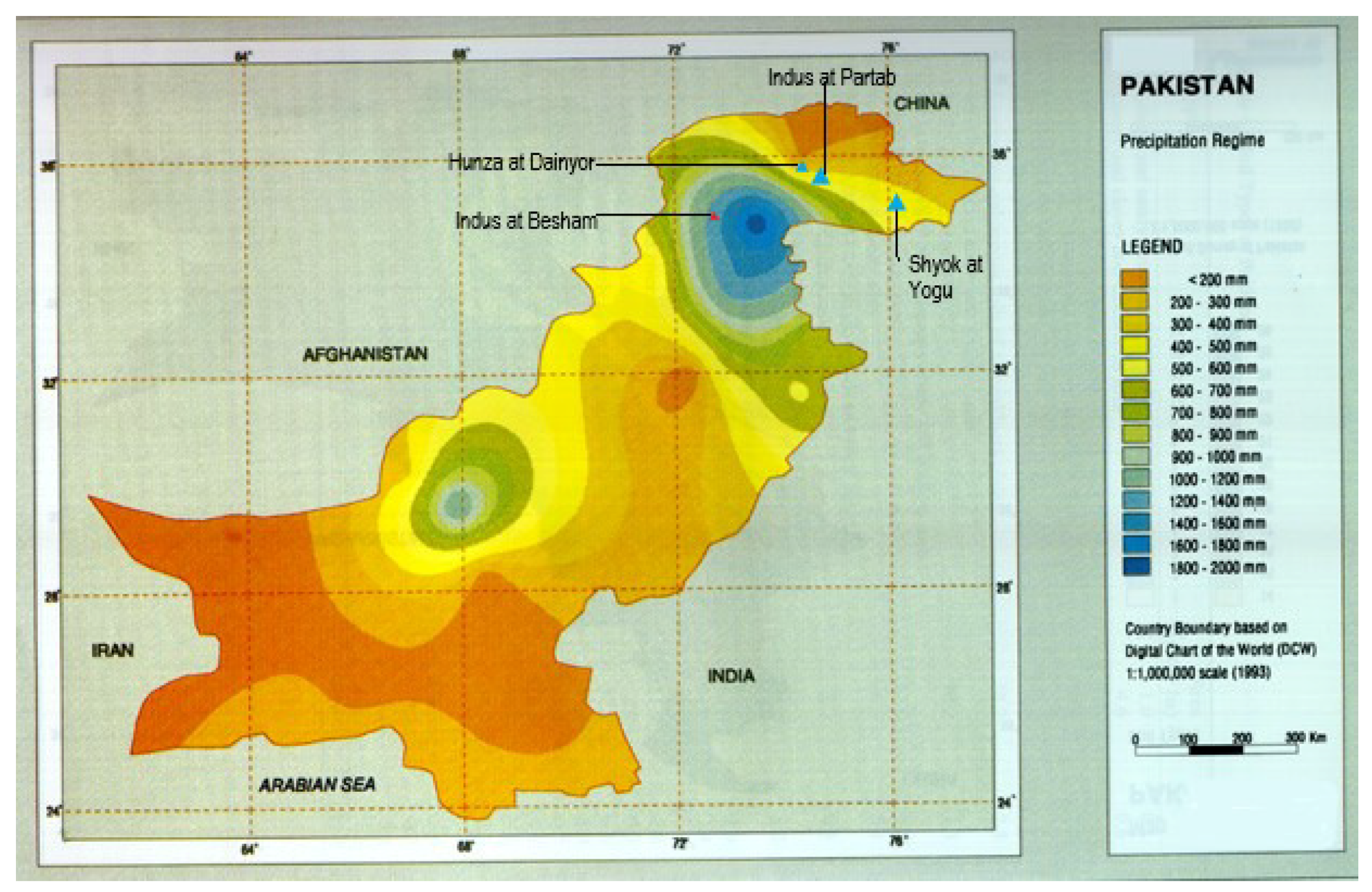
Figure 3.
Mean annual suspended sediment loads (SSLs) at (a) Yugo, (b) Dainyor, (c) Partab, and (d) Besham Qila stations used in the study.
Figure 3.
Mean annual suspended sediment loads (SSLs) at (a) Yugo, (b) Dainyor, (c) Partab, and (d) Besham Qila stations used in the study.

Figure 4.
Detailed coefficients of (DW1) two years, (DW2) four years, (DW3) eight years, and (DW4) sixteen years along with approximation coefficient (A4) of Dainyor. The figure shows that a change in magnitude of high and low SSC remains the same.
Figure 4.
Detailed coefficients of (DW1) two years, (DW2) four years, (DW3) eight years, and (DW4) sixteen years along with approximation coefficient (A4) of Dainyor. The figure shows that a change in magnitude of high and low SSC remains the same.
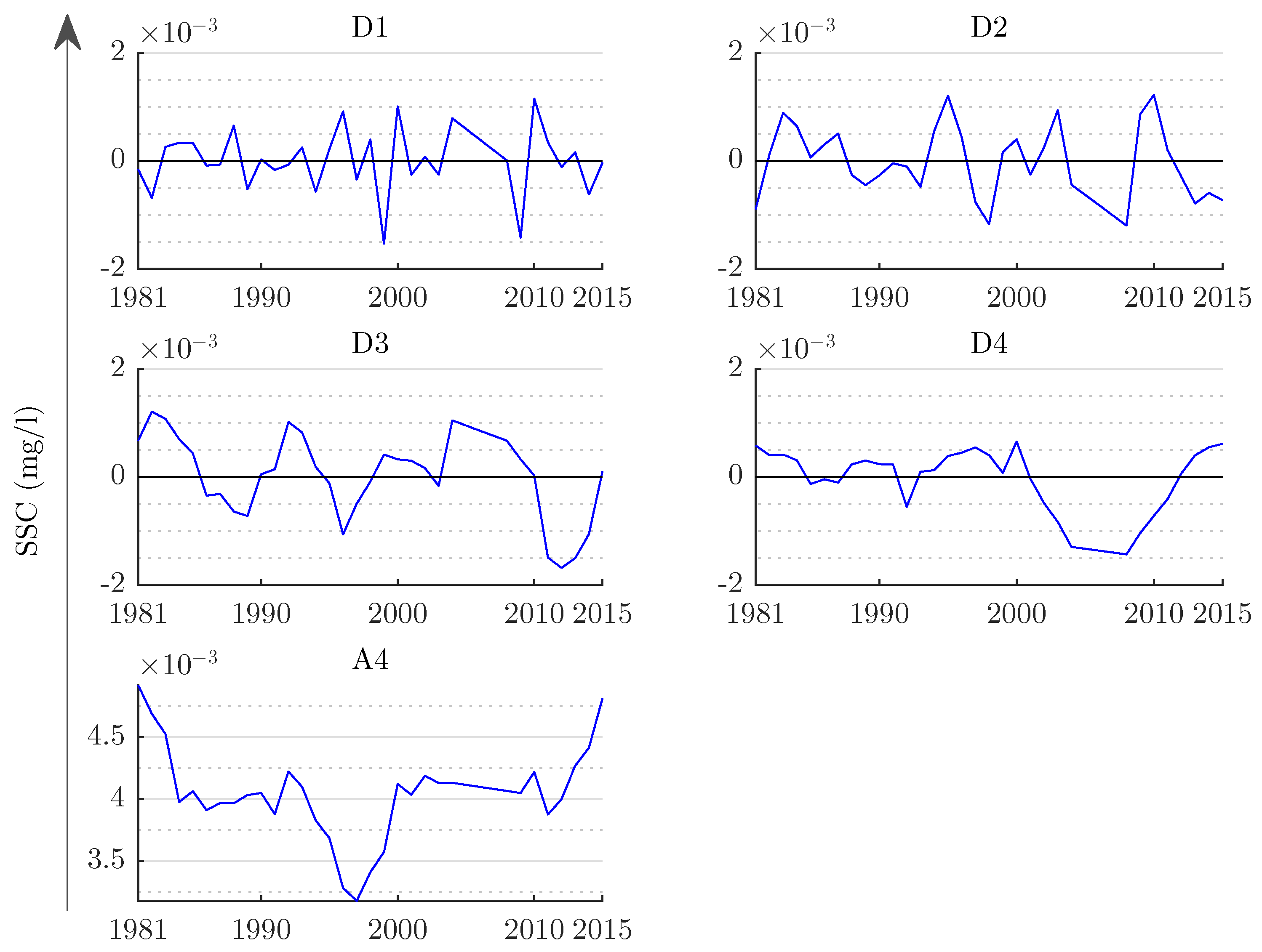
Figure 5.
Detailed coefficients of (DW1) two years, (DW2) four years, (DW3) eight years, and (DW4) sixteen years along with the approximation coefficient (A4) of Yugo are shown.
Figure 5.
Detailed coefficients of (DW1) two years, (DW2) four years, (DW3) eight years, and (DW4) sixteen years along with the approximation coefficient (A4) of Yugo are shown.
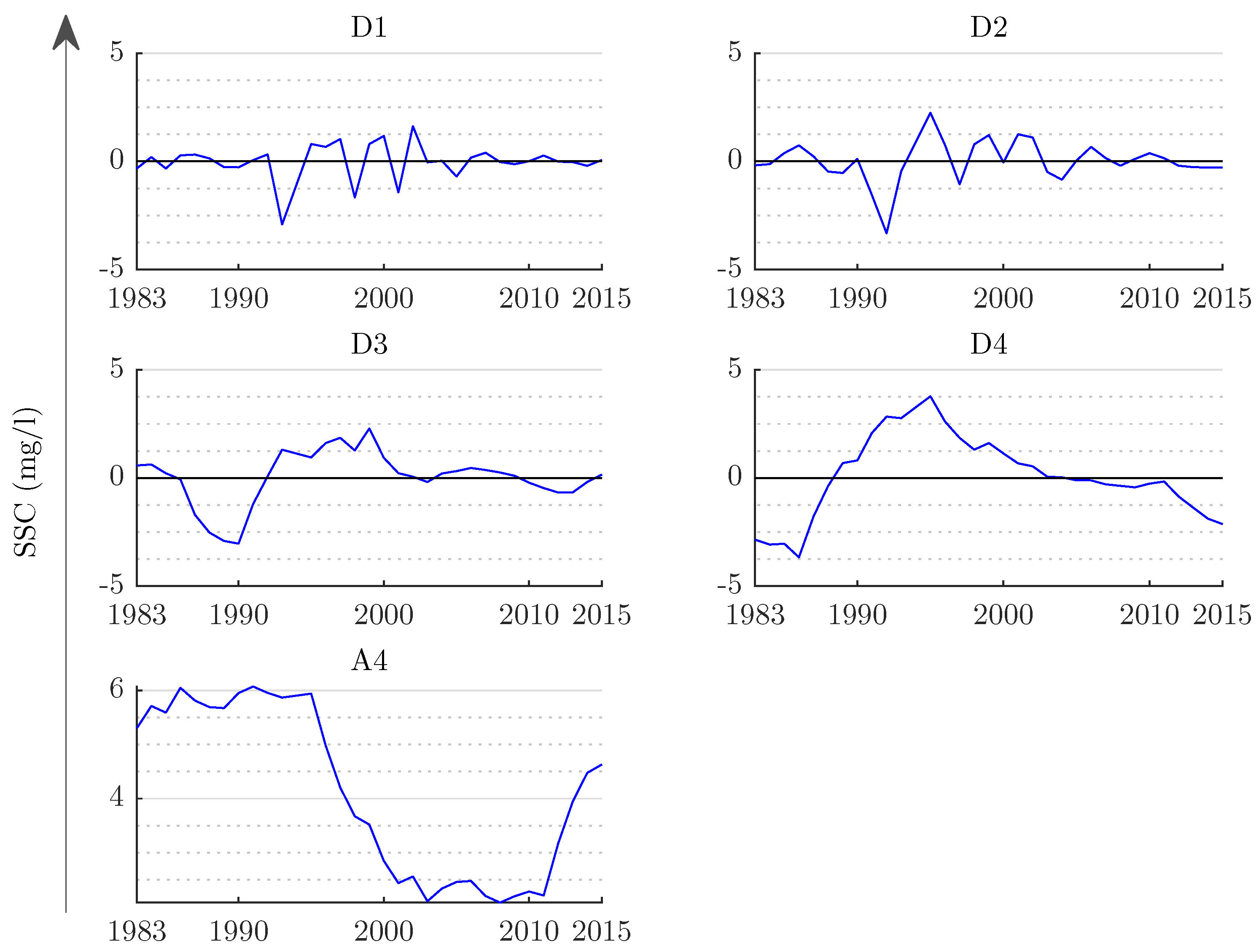
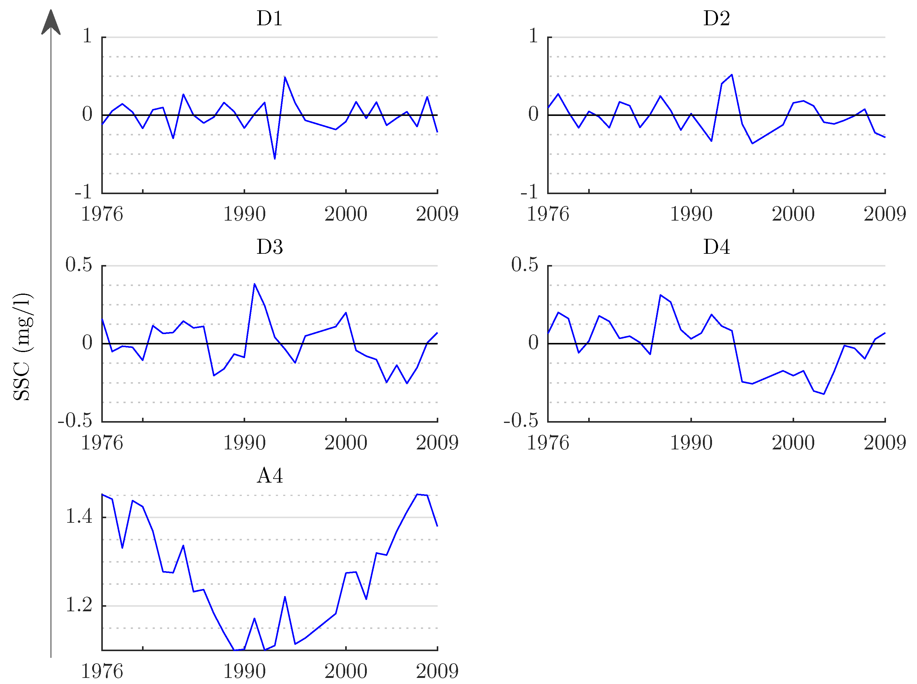
Figure 6.
Detailed coefficients of (DW1) two years, (DW2) four years, (DW3) eight years, and (DW4) sixteen years along with the approximation coefficient (A4) of Partab are shown.
Figure 6.
Detailed coefficients of (DW1) two years, (DW2) four years, (DW3) eight years, and (DW4) sixteen years along with the approximation coefficient (A4) of Partab are shown.

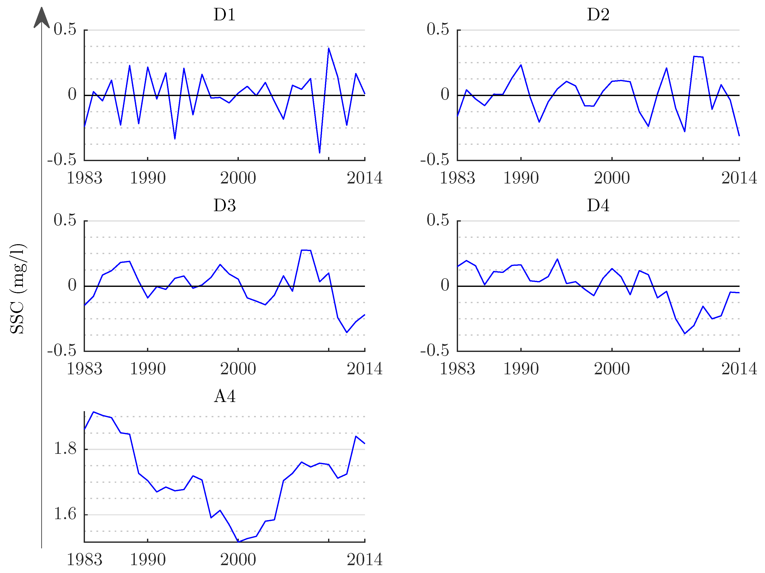
Figure 7.
Detailed coefficients of (DW1) two years, (DW2) four years, (DW3) eight years, and (DW4) sixteen years along with the approximation coefficient (A4) of Besham Qila are shown.
Figure 7.
Detailed coefficients of (DW1) two years, (DW2) four years, (DW3) eight years, and (DW4) sixteen years along with the approximation coefficient (A4) of Besham Qila are shown.


Table 1.
Data characteristics.
| Type | Dainyor | Yugo | Partab Bridge | Besham Qila |
|---|---|---|---|---|
| Data series | 1981–2015 | 1983–2015 | 1976–2009 | 1983–2014 |
| Max SSC (suspended sediment concentration) (mg/L) | 21,300 | 35,600 | 25,040 | 28,800 |
| Min SSC (mg/L) | 6 | 10 | 1 | 9 |
| Mean SSC (mg/L) | 1223 | 1330 | 2018 | 1179 |
| SD (standard deviation) SSC (mg/L) | 2397 | 4181 | 2950 | 1747 |
| Max discharge (m3/s) | 1792 | 1199 | 9287 | 18,071 |
| Min discharge (m3/s) | 22 | 859 | 168 | 362 |
| Mean discharge (m3/s) | 362 | 1041 | 2126 | 3221 |
| SD discharge (m3/s) | 397 | 103 | 2119 | 2978 |
Table 2.
Monthly Mann–Kendall (MK) test results with different wavelet decompositions for Dainyor, Yugo, Partab Bridge and Besham Qila (sign of MK statistic indicates trend type).
Table 2.
Monthly Mann–Kendall (MK) test results with different wavelet decompositions for Dainyor, Yugo, Partab Bridge and Besham Qila (sign of MK statistic indicates trend type).
| Jan | Feb | Mar | Apr | May | Jun | Jul | Aug | Sep | Oct | Nov | Dec | |
|---|---|---|---|---|---|---|---|---|---|---|---|---|
| Dainyor | ||||||||||||
| Original series: | 2.385 | 3.033 | 1.508 | −0.454 | −0.195 | −0.681 | −3.584 | −3.811 | −1.784 | −1.963 | 1.396 | 1.136 |
| D1 + A4 | 1.371 | 1.704 | 1.135 | 2.254 | 0.114 | −1.670 | −0.811 | −0.568 | 0.714 | −0.868 | 0.900 | 0.609 |
| D2 + A4 | 1.655 | 2.013 | 1.573 | 1.962 | 0.422 | −1.297 | −0.519 | −0.892 | 0.811 | −0.673 | 1.395 | 0.803 |
| D3 + A4 | 0.714 | 1.964 | 1.606 | 2.238 | 0.795 | −2.173 | −1.054 | −0.665 | 0.892 | −1.468 | 1.233 | 1.460 |
| D4 + A4 | 2.069 | 2.410 | 1.800 | 1.703 | 0.835 | −1.654 | −1.646 | −2.595 | 0.114 | −3.260 | 1.063 | −0.949 |
| D1 + D2 + A4 | 1.200 | 1.423 | 1.076 | 1.530 | 0.114 | −0.903 | −0.665 | −0.870 | 0.254 | −0.611 | 0.790 | 0.590 |
| D1 + D3 + A4 | 0.573 | 1.390 | 1.097 | 1.714 | 0.362 | −1.487 | −1.022 | −0.719 | 0.308 | −1.141 | 0.681 | 1.027 |
| D1 + D4 + A4 | 1.476 | 1.688 | 1.227 | 1.357 | 0.389 | −1.141 | −1.416 | −2.005 | −0.211 | −2.336 | 0.568 | −0.578 |
| D1 + D2 + D3 + A4 | 0.860 | 1.677 | 1.416 | 1.741 | 0.400 | −1.276 | −1.146 | −1.211 | 0.086 | −1.173 | 0.871 | 1.211 |
| D1 + D2 + D4 + A4 | 1.763 | 1.975 | 1.546 | 1.384 | 0.427 | 0.930 | −1.541 | −2.497 | −0.432 | −2.368 | 0.757 | −0.395 |
| D1 − D4 + A4 | 0.853 | 1.337 | 1.132 | 0.957 | 0.428 | −0.782 | −1.213 | 1.703 | −0.360 | −1.758 | 0.503 | 0.136 |
| D2 + D3 + A4 | 0.763 | 1.596 | 1.389 | 1.519 | 0.568 | −1.238 | −0.827 | −0.935 | 0.373 | −1.011 | 1.011 | 1.157 |
| D2 + D4 + A4 | 1.666 | 1.893 | 1.519 | 1.162 | 0.595 | −0.892 | −1.222 | −2.222 | −0.146 | −2.206 | 0.898 | −0.449 |
| D2 + D3 + D4 + A4 | 0.994 | 1.611 | 1.395 | 1.030 | 0.661 | −0.949 | −1.277 | −1.922 | −0.235 | −2.076 | 0.734 | 0.130 |
| D3 + D4 + A4 | 1.038 | 1.861 | 1.541 | 1.346 | 0.843 | −1.476 | −1.579 | −2.070 | −0.092 | −2.736 | 0.790 | −0.011 |
| Yugo | ||||||||||||
| Original series: | 0.573 | 0.238 | −0.341 | 1.897 | 0.325 | −0.2481 | −0.924 | −1.865 | −1.284 | 0.232 | 0.089 | 0.032 |
| D1 + A4 | - | - | −2.149 | −1.468 | −1.135 | −1.881 | −2.246 | −2.205 | - | - | - | −1.971 |
| D2 + A4 | - | - | −1.963 | −1.192 | −0.405 | −2.092 | −2.100 | −2.351 | - | - | - | −1.922 |
| D3 + A4 | - | - | −1.509 | −0.535 | −1.719 | −2.205 | −2.246 | −2.14 | - | - | - | −1.614 |
| D4 + A4 | - | - | −2.530 | 0.738 | −0.925 | -3.00 | −2.417 | −1.524 | - | - | - | −1.533 |
| D1 + D2 + A4 | - | - | −1.363 | −0.935 | −0.265 | −1.627 | −1.535 | −1.681 | - | - | - | −1.276 |
| D1 + D3 + A4 | - | - | −1.060 | −0.497 | −1.141 | −1.703 | −1.633 | −1.541 | - | - | - | −1.070 |
| D1 + D4 + A4 | - | - | −1.741 | 0.352 | −0.611 | −2.232 | −1.746 | −1.130 | - | - | - | −1.016 |
| D1 + D2 + D3 + A4 | - | - | −0.990 | −0.454 | −0.649 | −2.076 | −1.670 | −1.751 | - | - | - | −1.033 |
| D1 + D2 + D4 + A4 | - | - | −1.671 | 0.395 | −0.119 | −2.605 | −1.784 | −1.341 | - | - | - | −0.979 |
| D1 − D4 + A4 | - | - | −0.779 | 0.526 | −0.302 | −1.832 | −1.151 | −0.846 | - | - | - | −0.441 |
| D2 + D3 + A4 | - | - | −0.936 | −0.314 | −0.654 | −1.843 | −1.535 | −1.638 | - | - | - | −1.038 |
| D2 + D4 + A4 | - | - | −1.617 | 0.535 | −0.125 | −2.373 | −1.649 | −1.227 | - | - | - | −0.984 |
| D2 + D3 + D4 + A4 | - | - | −0.933 | 0.762 | −0.381 | −2.116 | −1.338 | −0.973 | - | - | - | −0.555 |
| D3 + D4 + A4 | - | - | −1.314 | 0.973 | −1.000 | −2.449 | −1.746 | −1.087 | - | - | - | −0.778 |
| Partab Bridge | ||||||||||||
| Original series: | 4.332 | 4.412 | 2.450 | 2.303 | −0.665 | 0.616 | −0.114 | 0.341 | 0.616 | 1.281 | 2.336 | 3.748 |
| D1 + A4 | 0.154 | 1.176 | 1.346 | 0.341 | 0.697 | 1.573 | 1.930 | 0.811 | 0.478 | −0.592 | −1.802 | −0.365 |
| D2 + A4 | 0.479 | 0.957 | 1.046 | 0.584 | 0.122 | 1.589 | 1.557 | 0.649 | 0.154 | −0.381 | −1.218 | 0.105 |
| D3 + A4 | 1.275 | 1.217 | 1.144 | 1.200 | 0.884 | 1.703 | 1.362 | 1.005 | 1.014 | 0.463 | 0.024 | 0.479 |
| D4 + A4 | 2.378 | 2.150 | 1.873 | 1.306 | −1.200 | 0.957 | 1.914 | 0.373 | 0.592 | 1.679 | −0.219 | 1.614 |
| D1 + D2 + A4 | 0.384 | 0.844 | 1.130 | 0.297 | −0.027 | 1.076 | 1.324 | 0.622 | 0.270 | −0.341 | −0.969 | 0.092 |
| D1 + D3 + A4 | 0.915 | 1.017 | 1.195 | 0.708 | 0.481 | 1.151 | 1.195 | 0.859 | 0.843 | 0.222 | −0.141 | 0.341 |
| D1 + D4 + A4 | 1.650 | 1.639 | 1.682 | 0.779 | −0.908 | 0.654 | 1.562 | 0.438 | 0.562 | 1.033 | −0.303 | 1.098 |
| D1 + D2 + D3 + A4 | 1.196 | 1.076 | 1.427 | 0.778 | −0.011 | 1.178 | 1.232 | 0.941 | 0.795 | 0.276 | 0.092 | 0.676 |
| D1 + D2 + D4 + A4 | 1.931 | 1.698 | 1.914 | 0.849 | −1.400 | 0.681 | 1.600 | 0.519 | 0.514 | 1.087 | −0.070 | 1.433 |
| D1 −D4 + A4 | 1.646 | 1.158 | 1.327 | 0.798 | −0.830 | 0.470 | 0.905 | 0.503 | 0.623 | 1.022 | 0.594 | 1.210 |
| D2 + D3 + A4 | 1.131 | 0.871 | 0.995 | 0.870 | 0.097 | 1.162 | 0.946 | 0.751 | 0.627 | 0.362 | 0.249 | 0.654 |
| D2 + D4 + A4 | 1.866 | 1.493 | 1.481 | 0.941 | −1.292 | 0.665 | 1.314 | 0.330 | 0.346 | 1.174 | 0.087 | 1.411 |
| D2 + D3 + D4 + A4 | 2.009 | 1.294 | 1.334 | 1.066 | −0.957 | 0.576 | 0.916 | 0.486 | 0.653 | 1.343 | 0.860 | 1.497 |
| D3 + D4 + A4 | 2.398 | 1.666 | 1.546 | 1.352 | −0.784 | 0.741 | 1.184 | 0.568 | 0.919 | 1.736 | 0.915 | 1.660 |
| Besham Qila | ||||||||||||
| Original series: | 1.721 | 2.794 | 1.347 | 0.714 | 0.890 | −0.211 | −1.022 | −2.060 | −2.838 | −0.925 | 0.455 | 0.227 |
| D1 + A4 | 0.081 | 1.647 | 0.982 | −1.760 | −0.835 | −0.949 | − 1.297 | −1.362 | − 1.225 | −1.468 | −1.501 | − 0.747 |
| D2 + A4 | 0.235 | 1.769 | 0.641 | −1.330 | − 0.584 | −0.892 | −1.695 | −1.930 | −1.565 | −1.225 | −1.477 | − 0.511 |
| D3 + A4 | 0.657 | 1.899 | 0.138 | −0.835 | −0.211 | −0.997 | −2.214 | −2.343 | −1.743 | −1.760 | −1.143 | −0.730 |
| D4 + A4 | 0.008 | 1.712 | 1.509 | −1.898 | −2.805 | −1.038 | −2.546 | −2.659 | −2.879 | −2.320 | −2.410 | −3.125 |
| D1 + D2 + A4 | 0.325 | 1.331 | 0.368 | −0.687 | −0.195 | −0.616 | −0.822 | −1.065 | −0.800 | −0.671 | −0.611 | −0.141 |
| D1 + D3 + A4 | 0.606 | 1.417 | 0.032 | −0.357 | 0.054 | −0.687 | − 1.168 | −1.341 | −0.919 | −1.027 | −0.389 | −0.287 |
| D1 + D4 + A4 | 0.173 | 1.293 | 0.946 | −1.065 | −1.676 | −0.714 | −1.389 | −1.551 | −1.676 | −1.401 | 1.234 | −1.883 |
| D1 + D2 + D3 + A4 | 0.877 | 1.650 | −0.254 | 0.130 | 0.416 | −0.670 | −1.124 | −1.497 | −0.903 | −0.719 | 0.000 | 0.070 |
| D1 + D2 + D4 + A4 | 0.444 | 1.526 | 0.660 | −0.579 | −1.314 | −0.697 | −1.346 | −1.708 | −1.660 | −1.093 | −0.844 | −1.526 |
| D1 − D4 + A4 | 0.597 | 1.107 | 0.023 | 0.143 | −0.422 | −0.451 | −0.989 | −1.284 | −1.057 | −0.685 | −0.139 | −0.789 |
| D2 + D3 + A4 | 0.709 | 1.499 | −0.195 | −0.070 | 0.222 | −0.649 | −1.432 | −1.719 | −1.146 | −0.865 | −0.373 | −0.130 |
| D2 + D4 + A4 | 0.276 | 1.374 | 0.719 | −0.779 | −1.508 | −0.676 | −1.654 | −1.930 | −1.903 | −1.239 | −1.217 | −1.726 |
| D2 + D3 + D4 + A4 | 0.621 | 1.270 | 0.073 | 0.028 | −0.673 | −0.547 | −1.468 | −1.772 | −1.504 | −0.965 | −0.454 | −1.136 |
| D3 + D4 + A4 | 0.557 | 1.461 | 0.384 | −0.449 | −1.259 | −0.746 | −2.000 | −2.205 | −2.022 | −1.595 | −0.995 | −1.872 |
Bold values signify a trend at 95 percent significance level (critical valuable = 1.96). The dash (−) signifies that length of data inadequate to run discrete wavelet transform (DWT).
© 2018 by the authors. Licensee MDPI, Basel, Switzerland. This article is an open access article distributed under the terms and conditions of the Creative Commons Attribution (CC BY) license (http://creativecommons.org/licenses/by/4.0/).
Share and Cite
MDPI and ACS Style
Tarar, Z.R.; Ahmad, S.R.; Ahmad, I.; Majid, Z. Detection of Sediment Trends Using Wavelet Transforms in the Upper Indus River. Water 2018, 10, 918. https://doi.org/10.3390/w10070918
AMA Style
Tarar ZR, Ahmad SR, Ahmad I, Majid Z. Detection of Sediment Trends Using Wavelet Transforms in the Upper Indus River. Water. 2018; 10(7):918. https://doi.org/10.3390/w10070918
Chicago/Turabian StyleTarar, Zeeshan Riaz, Sajid Rashid Ahmad, Iftikhar Ahmad, and Zahra Majid. 2018. "Detection of Sediment Trends Using Wavelet Transforms in the Upper Indus River" Water 10, no. 7: 918. https://doi.org/10.3390/w10070918
Note that from the first issue of 2016, this journal uses article numbers instead of page numbers. See further details here.