A Dynamic Study of a Karst Spring Based on Wavelet Analysis and the Mann-Kendall Trend Test
by
Liting Xing
1,2, 
Linxian Huang
1,2,*,
Guangyao Chi
1,
Lizhi Yang
3,
Changsuo Li
4 and
Xinyu Hou
1 1
School of Water Conservancy and Environment, University of Jinan, Jinan 250022, China
2
Engineering Technology Institute for Groundwater Numerical Simulation and Contamination Control, Jinan 250022, China
3
Shandong Institute of Geological Survey, Jinan 250000, China
4
Shandong Provincial Geo-mineral Engineering Exploration Institute, Jinan 250014, China
*
Author to whom correspondence should be addressed.
Water 2018, 10(6), 698; https://doi.org/10.3390/w10060698
Submission received: 15 April 2018
/
Revised: 24 May 2018
/
Accepted: 24 May 2018
/
Published: 28 May 2018
(This article belongs to the Section Water Resources Management, Policy and Governance)
Abstract
:Over the last 40 years, declining spring water flow rates have become a typical feature of karst springs in Northern China. Wavelet analysis, the Mann-Kendall trend test and the mutation test were used to analyze dynamic monitoring data of groundwater levels and atmospheric precipitation in the Jinan karst spring area, from 1956 to 2013, to study hydrological responses to atmospheric precipitation over one-year periods. Results from this analysis show that: (1) Atmospheric precipitation and the spring water level displayed multi-scale change characteristics, having two very similar cycles of change of 16 and 12 years. This finding shows that atmospheric precipitation generates a direct impact on the level of spring water. (2) From 1956 to 2013, the groundwater level in the Jinan spring area had a significant downward trend (0.65 m/10a). Precipitation recorded an increasing trend (12.65 mm/10a), however this was not significant. The weight of the influencing factors of the spring dynamic therefore changed due to the influence of human factors. (3) A mutation of atmospheric precipitation occurred in 1999, after which annual precipitation increased. Results for the mutation of the groundwater level showed an initial change in 1967. After this change the water level continued to decrease before rapidly increasing after 2004. The future trend of the spring water level should be maintained with consistent precipitation (having an upward trend), indicating that atmospheric precipitation is not the only factor affecting the dynamics of the spring. (4) Different periods were identified on the multiple regression model. The main influencing factors on groundwater level over the past 58 years were identified as a transition from precipitation to artificial mining. These results also validate the suitability and reliability of using wavelet analysis and the Mann-Kendall test method to study groundwater dynamics; these results provide a reference for the future protection of the Jinan City spring.
1. Introduction
Atmospheric precipitation is an important factor affecting groundwater dynamics and periodic precipitation affects groundwater levels by ensuring a certain period of change [1,2,3,4,5]. Baotu spring, located in Jinan city, is not only historically very important in China, it is renowned across the world. Karst water from the springs in the Jinan area has historically been the main water source. However, with economic and population development, the volume of groundwater exploitation has sharply increased in this area since the early 1970s, and artificial exploitation has had a tremendous impact on spring water supply. In 1972 Baotu spring seasonal stopped flowing, creating great concern for local inhabitants. In order to resume spring flow it was stipulated in 2003 that large-scale exploitation of groundwater should be prohibited near the spring area. Groundwater exploitation was reduced from 800,000 m3/d to 100,000 m3/d, and 90% of the urban water supply was instead taken from the Yellow River (this water being classed as inferior to the spring water). Although groundwater exploitation has declined drastically in recent years, there is still a threat of spring water discontinuity during the dry season. With issues relating to flow levels in the spring not being resolved with the substantial reduction in exploitation, we can infer that influencing factors on spring dynamics due to anthropogenic activities have changed.
In order to sustainably develop and utilize groundwater resources and protect the groundwater environment, a substantial volume of research has been undertaken examining the variation of atmospheric precipitation and groundwater. Proposed methods include, for example, the regression method [6,7], time series methods, spectrum analysis, artificial neural network, Gray analysis, dynamic neural network models, and the kernel function methods [8,9,10,11,12]. These investigations have increased precision in the law of dynamic change for groundwater and promoted the development of groundwater science. However, the loose rock type water and karst fissure water dynamics are quite different. A karst aqueous medium is highly heterogeneous and anisotropic, and its water circulation process is complex, resulting in karst fissures having a strong water flow [13,14]. This has led to an increase in laboratory-based physical model experiments investigating karst water flow movement [15,16]. However, due to limitations in experimental devices, it is very difficult to reproduce the complex hydrogeological structures and their scale effects in the laboratory. At the same time, the heterogeneity of a karst aqueous medium cannot meet the requirement of generalization of hydrogeological conditions. In order to understand the law of groundwater dynamic variation, karst fissures, karst pipelines, dissolved pores and large fissures were generalized and numerically sampled to simulate karst hydrodynamic characteristics [17,18,19]. However, hydrogeological parameters required for the numerical simulation of groundwater are a function of space-time coordinates. Due to current limitations, the complex function relationship between parameters and geological bodies cannot be accurately described, thus leading to uncertainty in identifying hydrogeological parameters. Errors present in model parameters therefore reflect our lack of understanding of the hydrogeological structure. In order to avoid issues related to physical models and the numerical simulation of a heterogeneous aquifer system, a large body of research examined relationships between precipitation and groundwater level, precipitation and groundwater recharge [20], and the characteristics of time lag of precipitation on the dynamic of groundwater [21,22] using the Morlet wavelet method [23], the Mann-Kendall trend test (M-K) [24] and the Hurst index method. The wavelet analysis method was used to study the evolution of annual precipitation in Pelotas, Brazil from 1894 to 1995. The average annual precipitation, ENSO (El Niño phenomenon), and a two-year oscillation period were analyzed using cross-spectrum analysis [25]. By sorting out the precipitation data from the Uccle station in Belgium from 1898 to 2002 for 105 years, the characteristics of annual, seasonal, and monthly precipitation were analyzed [26]. Based on the monthly precipitation data of the Iberian Peninsula from 1921 to 1995, the Mann-Kendall trend analysis was used to analyze the trend of precipitation [27]. Mann-Kendall method is used to analyze precipitation change in the Yangtze River basin [28].The study found that the precipitation in the continental United States showed a significant increase and the spatial distribution was very uneven [29]. The research found that the changing trend of precipitation in Japan is: The trend of heavy precipitation is increasing and the weak precipitation is decreasing [30]. By analyzing the data of rainfall in Singapore from 1981 to 2010, the results show that Singapore’s annual precipitation, daily precipitation, and hourly precipitation all show an increasing trend [31]. Among them, the maximum daily precipitation has the fastest growth rate. At the same time, the characteristics of changes in precipitation across the globe have regional differences. The study found that both the heavy precipitation and the weak precipitation in the western continental Europe and the United States showed an increasing trend, while the medium-intensity precipitation showed a decreasing trend. However, the strong precipitation in East Asia showed an increasing trend, while the medium-intensity precipitation and the weak precipitation both showed a decreasing trend [32,33]. Having established a model to analyze the spatial variability of precipitation in Desert Steppe in West Africa [34]. Current studies have shown that stochastic theory is an effective method to study the groundwater dynamics in a heterogeneous aquifer system. The Morlet wavelet analysis method has the function of time-frequency multiresolution. The advantage of this method is that it can clearly reveal many types of change cycles in a time series, reflecting the changing characteristics of a system under different time scales, and it can qualitatively analyze the future development trend of the system. Therefore, wavelet analysis can be used to identify multi-scale features of atmospheric precipitation and spring water level changes [35,36,37,38,39,40,41]. In time series trend analysis, the M-K test is a non-parametric test method which is recommended and widely used by the World Meteorological Organization. The M-K test does not require samples to follow a certain distribution and it is not affected by a few abnormal values. This method is suitable for non-normal distributed data series, such as hydrological and meteorological data sets [42,43,44,45]. The M-K trend test and mutation detection methods are simple to compute and can be used to study the effects of atmospheric precipitation on water level sequences.
In order to provide a reference for the protection of the Jinan City spring, in this study we used time serial analysis involving wavelet analysis and the M-K nonparametric test; analyzed the sequence of precipitation and spring water levels in Jinan city over the last 58 years; examined the multiscale features of atmospheric precipitation and spring water level changes; and examined lag time of water levels relative to precipitation.
2. Materials and Methods
2.1. The Background Conditions of the Study Area
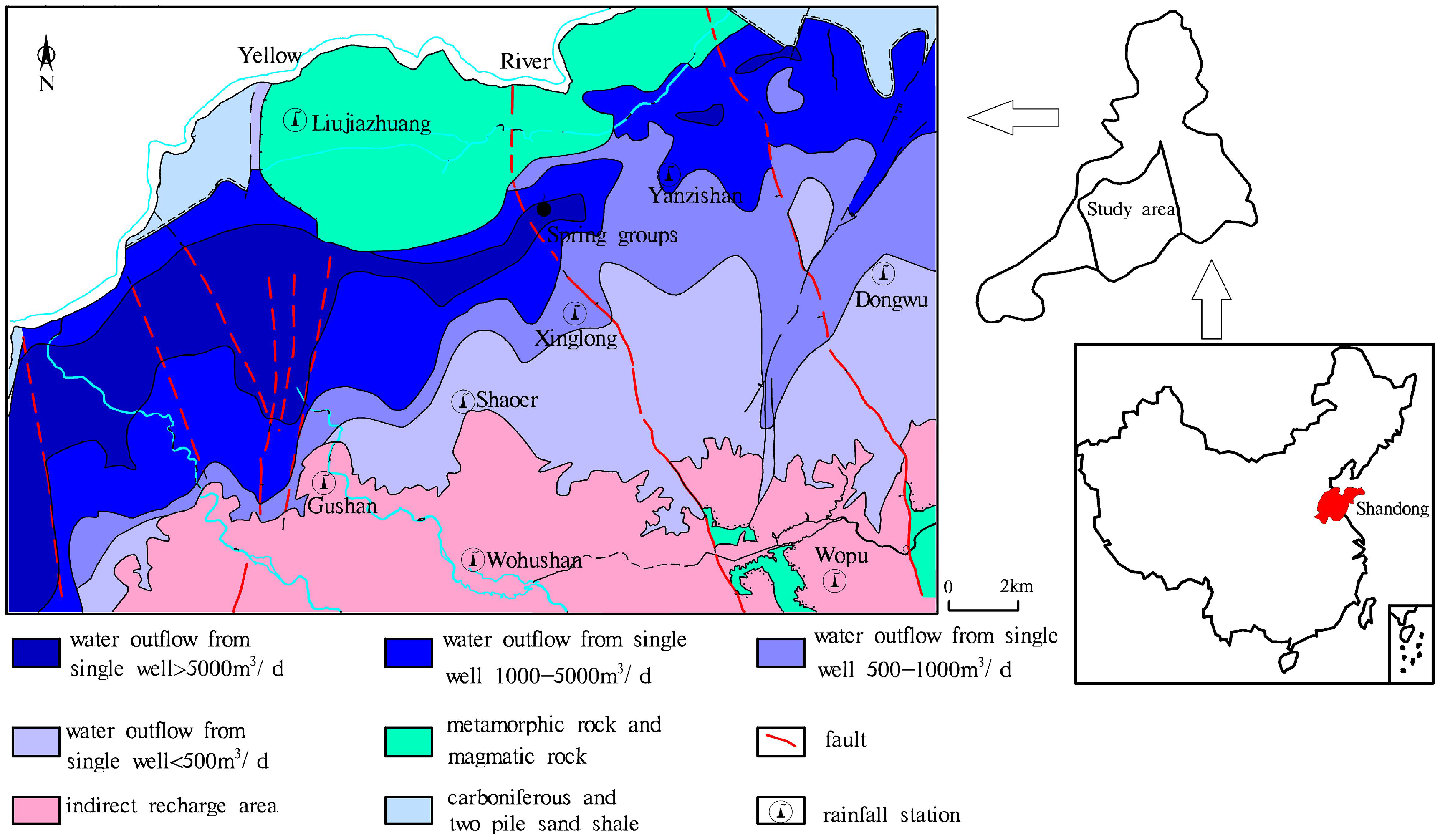
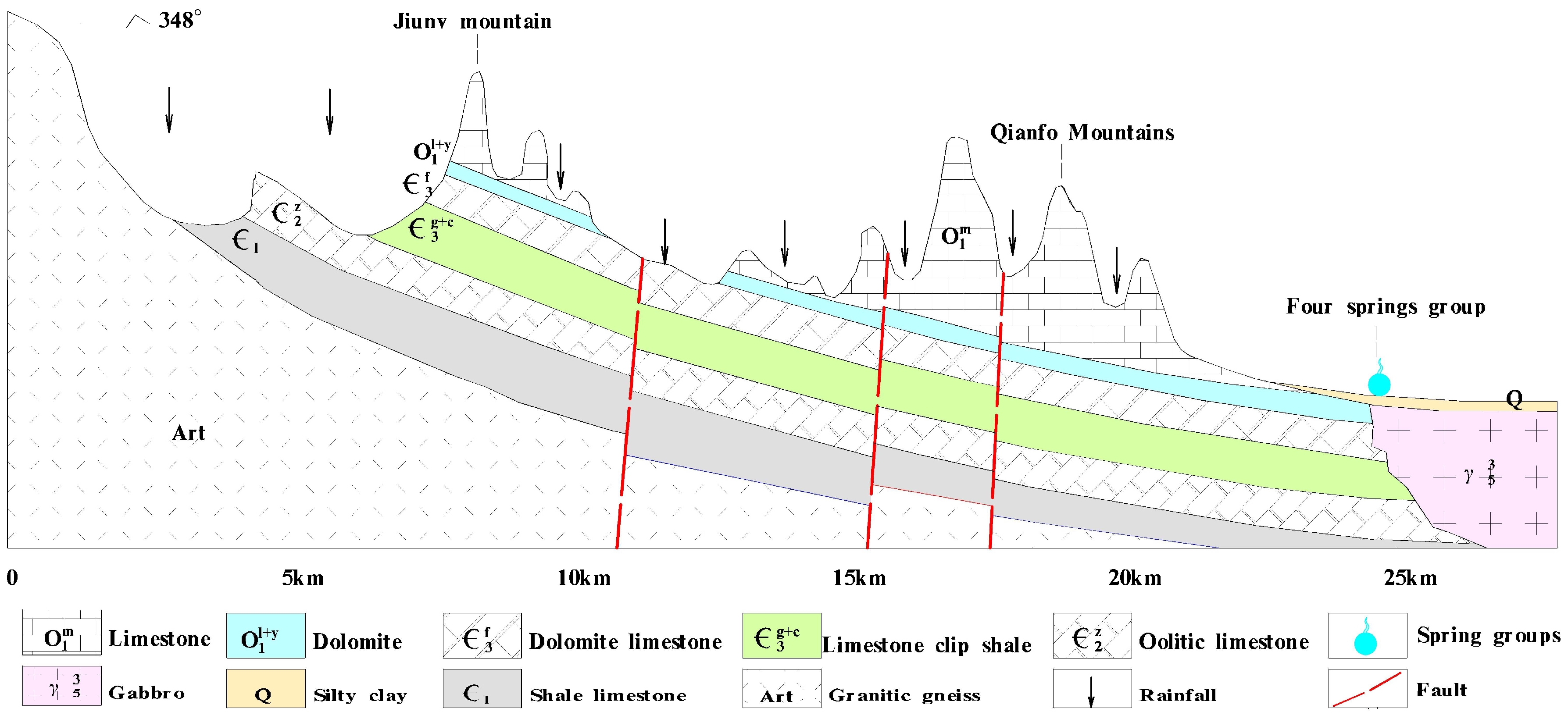
Jinan spring field is located in central and western Shandong Province. It has a warm temperate continental monsoon climate, an annual average temperature of 14.3 °C (1956–2013), and an average annual evaporation of 1500~1900 mm (1956–2013). Mean annual precipitation is around 676.94 mm (1956–2013), and the area has an uneven distribution of precipitation during the year, with about 73% of annual rainfall occurring from June to September. Jinan is located on the northern edge of the Shandong Mountains. The terrain is high in the south and low in the north, the south being the crystalline basement of the former Sinian gneisses. The Cambrian-Ordovician strata are exposed, ranging from old to new northwards, and the Yanshanian Magmatic rock is distributed in the north (Figure 1). The particular topography and geological structure in this area results in karst water in the southern mountain area to be recharged by atmospheric precipitation. The direction of movement of the karst water, the direction of the topography and the direction of the stratum are generally consistent, moving from the south to the north. As the karst water moves to the north, it is blocked by magmatic rocks. The groundwater becomes enriched at this point and, due to favorable terrain and geology, it reaches the surface as a spring (Figure 2). Atmospheric precipitation has been confirmed as the origin of the groundwater in the spring using isotopic analysis [46]. The dynamics of the groundwater level is affected by many factors, such as precipitation, artificial mining and local topography [6,47].
2.2. Data
Annual precipitation data from Jinan City (1956 to 2013) and average spring water levels (1959 to 2013) were selected as the data sources for our study. A section of the precipitation data was derived from observed data from the Jinan Station, station number 54,823 on the China Meteorological Data Network, this station being located in the Jinan spring field. The data of groundwater level was collected from manual observation and automatic monitoring observation; the volume of exploitation was from the water plant measurement data.
2.3. Periodic Inspection Method
By using Morlet wavelet as the basic wavelet, a continuous wavelet transform was used to analyze the multi-time scale features of annual precipitation and groundwater levels. This method also enabled the future development trend of spring field precipitation and groundwater levels to be qualitatively estimated. This technique, initially developed to analyze seismic data, has a good local analysis method in both the time and frequency domain. This method is defined as an arbitrary equation. More detailed descriptions of this method are introduced in References [48,49,50]:
where Wf(a, b) is the wavelet transform coefficient; f(t) is a signal or square-integrable function; a is the scaling scale; b is the translation parameter; and is the complex conjugate function of . Most of the time-series data observed in geosciences are discrete, and the function is f(kΔt) (k = 1, 2, ..., N); Δt is the sampling interval. The discrete wavelet transform of Equation (1) was:
2.4. Trend Test Method
Trend analysis using the M-K test supposes that H0 (unilateral test) represents the time series (x1, x2, …, xn) and is independent and identically distributed with no trend. Suppose that H1 (bilateral test) representing the data distribution of the time series is different, and the statistical variable S to be tested is calculated as follows:
where,
S is normal distribution. If the mean is 0, then the variance is:
where t is the range of any given node. When n > 10, Zc converges to a normal distribution and is calculated by:
In the bilateral trend test, if |Zc| > Z1 − α/2 is rejected at the given α confidence level, the original hypothesis H0 is rejected, i.e., there is a clear upward or downward trend of the time series data at the α confidence level. ±Z1 − α/2 is the standard normal distribution (1 − α/2) quantile, and α is the test’s confidence level. The size of the trend can be expressed using the Kendall inclination β, which is calculated as follows:
where 1 < j < i < n; β denotes the slope which is positive numbers with an upward trend and negative numbers with a downward trend. The larger the value of β, the more obvious the trend changes.
2.5. Mutation Test Method
In addition to trend analysis, the M-K method can also be used to test for mutation. This method is very effective for verifying a change of state from a relatively stable state to another state. For a time series x with n sample sizes, construct an order column
where,
It can be seen that the rank sequence Sk is the cumulative number of times the value of i at the moment i is greater than the number of values at time j. Under the assumption of random independence of time series, define statistics:
where UF1 = 0; E(Sk) and Var(Sk) are the mean and variance of the cumulative number Sk, respectively. This value is calculated when x1, x2, …, xn are independent and have the same continuous distribution as:
UFi is a standard normal distribution, which is a sequence calculated according to time series x order x1, x2, …, xn. Given a significance level a, in comparison with the data in the known normal distribution table, and if UFi > Ua, then significant changes exist in the trend. This method can also be applied to the inverse sequence of the time series, and the above procedure can be repeated by xn, xn−1, …, x1, thus making UFk = −UBk, k = n, n − 1, …, UB = 0. Given the significance level α, the two curves of UFk and UBk and the significant horizontal line are plotted on the same graph. If the values of UFk and UBk are greater than 0, then the sequence shows an upward trend; values below 0 indicate a downward trend. When the value exceeds the critical line, this indicates that the rising or falling trend is significant. The range beyond the critical line is defined as the time zone of mutation. If the UFk and UBk curves appear on an intersection point, and the intersection point is between the critical line, then the intersection point corresponds to the time the mutation begins. More detailed descriptions of this method are introduced in Reference [51].
3. Results
3.1. General Characteristics of Atmospheric Precipitation and Spring Water Level
From 1959 to 2013, the annual average groundwater level of the Jinan Spring Group was 27.75 m, and the average annual precipitation was 676.94 mm. Results in Figure 3 show that the groundwater level can be divided into four stages: 1959 to 1964: During this period spring water was in a state of high flow and had a high water level, 1965 to 1989: Flow from the spring declined and the groundwater level recorded a significant decline, 1990 to 2002: This period was regarded as the spring seasonal outflow/low water level fluctuation stage, 2003 to 2013: This stage recorded recharge of the artificial groundwater and was characterized by the spring flowing during this period. Analysis of these four phases indicated that factors influencing groundwater level in the Jinan spring area are dynamic and changeable. The main causes of groundwater level changes in the early study period were found to be linked to a change of atmospheric precipitation and artificial exploitation. Since 2003, due to artificial groundwater recharge, a reduction in groundwater exploitation, precipitation and artificial mining, the dynamic changes in the groundwater levels have become more complicated.
3.2. Atmospheric Precipitation and Spring Water Level Cyclical Changes
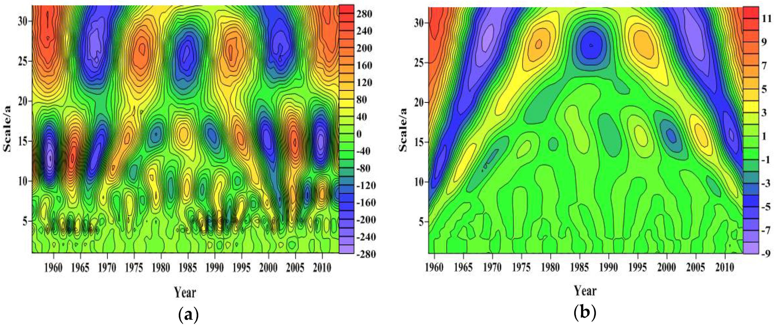
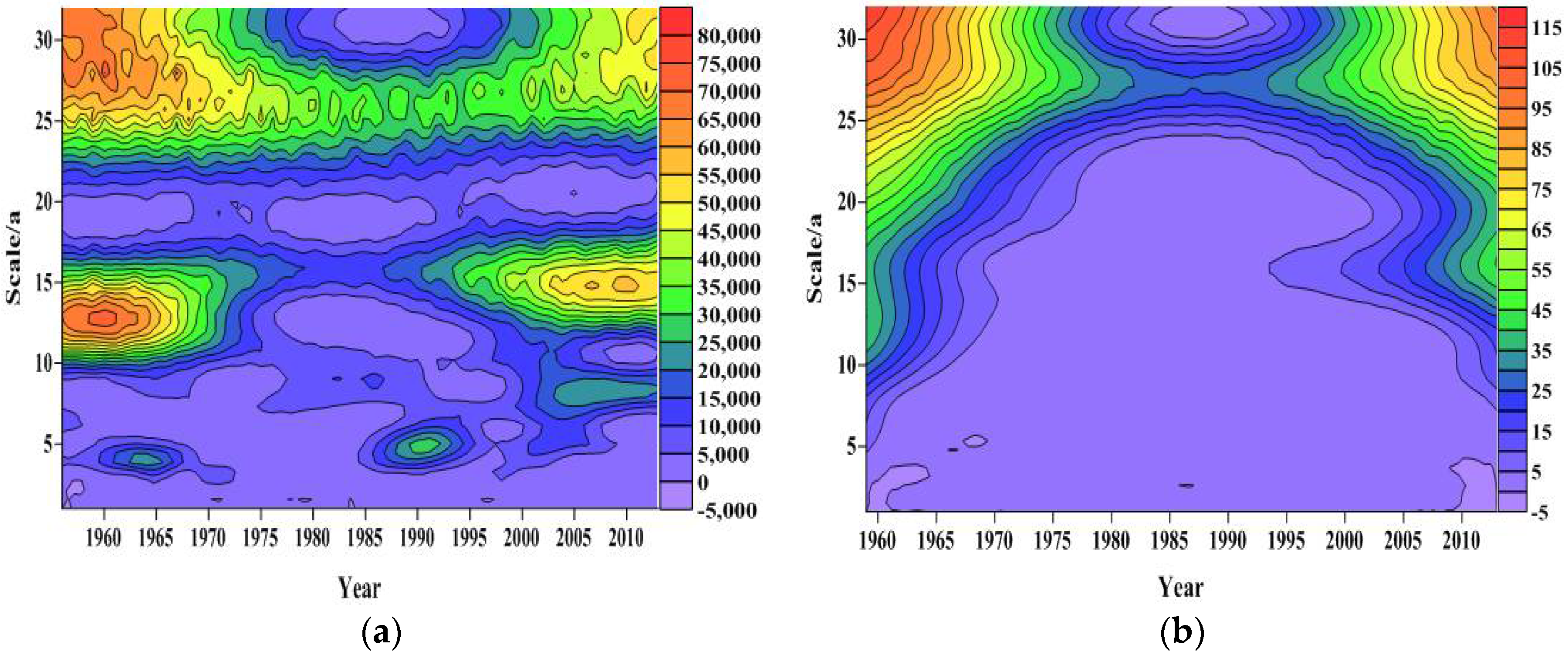
Although the distribution of precipitation in Jinan was uneven (Figure 3), a relationship exists between the spring water level and precipitation. The Morlet continuous complex wavelet transform was selected to analyze the multi-time scale features of atmospheric precipitation and the spring time series. Our results show that there were multiple historic time-scale features for atmospheric precipitation and spring water level. Precipitation time series results indicated three types of scale for periodic variation: 25–32 years, 10–15 years and 3–9 years (Figure 4a). In the 25–32 year scale, it appeared to be standard alternating three shocks in the dry season and the flood season; in the 10–15 year scale, there was the standard five shocks.The periodic changes of these two scales show a very stable and global trend throughout the analysis period. However, the period change of 3–9 years was more stable after 1985. A periodic variation of spring water level between the scales of 25–32 and 10–18 years was identified (Figure 4b). In the 25–32 year scale, the standard secondary shocks of fuming and withering appeared; in the 10–18 year standard secondary shocks were also identified. Meanwhile, the periodic variations of these two scales are very stable in the whole analysis period and it is global.
During the evolution of annual precipitation in the spring region, the maximum value of the time-scale was 25–32 years, and the most obvious change occurred during this time-scale, followed by the periodic changes in the 10–20 year time-scale. Periodic changes in other time-scales were smaller (Figure 5a). During the evolution of the spring water level during the spring period, the maximum value of the time-scale was 25–32 years, and the most obvious change occurred in this time-scale, followed by the periodic variation of 10–18 years (Figure 5b).
The spring field precipitation has the strongest energy and the most significant period in the 25–32 year time-scale, occupying almost the entire time domain of the study. However, energy on the 10–15 year time-scale is weak and periodic variation is localized (Figure 6a). The spring had the highest energy in the 25–32 year time-scale, this being the most significant period, which occupied almost the entire time domain of the study (Figure 6b).
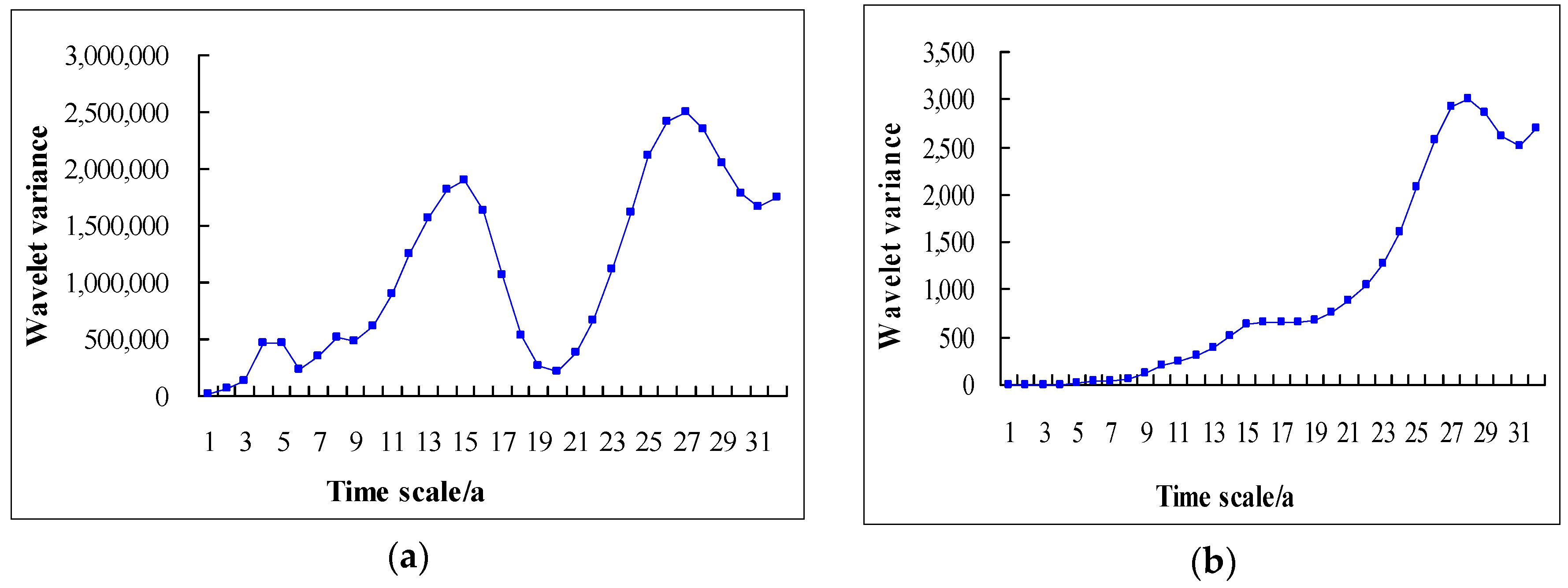
Four obvious peaks in the wavelet variance map of spring precipitation (Figure 7a) were identified, corresponding to the time-scales of 27, 15, 8 and 5 years, of which the maximum peak corresponded to a 27-year time-scale. This result indicates that the strongest periodic oscillation in 27 years was the first main period of annual precipitation change in the spring area. The 15-year time-scale corresponds to the second peak, which is the second main period of annual precipitation change, and the third and fourth peak correspond to 8-year and 5-year time-scales, respectively, which are in turn the third and fourth main cycles of annual spring precipitation. The fluctuations of these four periods control the variation of annual precipitation over the entire time domain. There are two obvious peaks in the wavelet variance map of the spring water level (Figure 7b), corresponding to the 27-year and 15-year time-scales in succession. The 27-year period is the first spring water level change event and the 15-year period is the second main cycle of change for the spring water level.
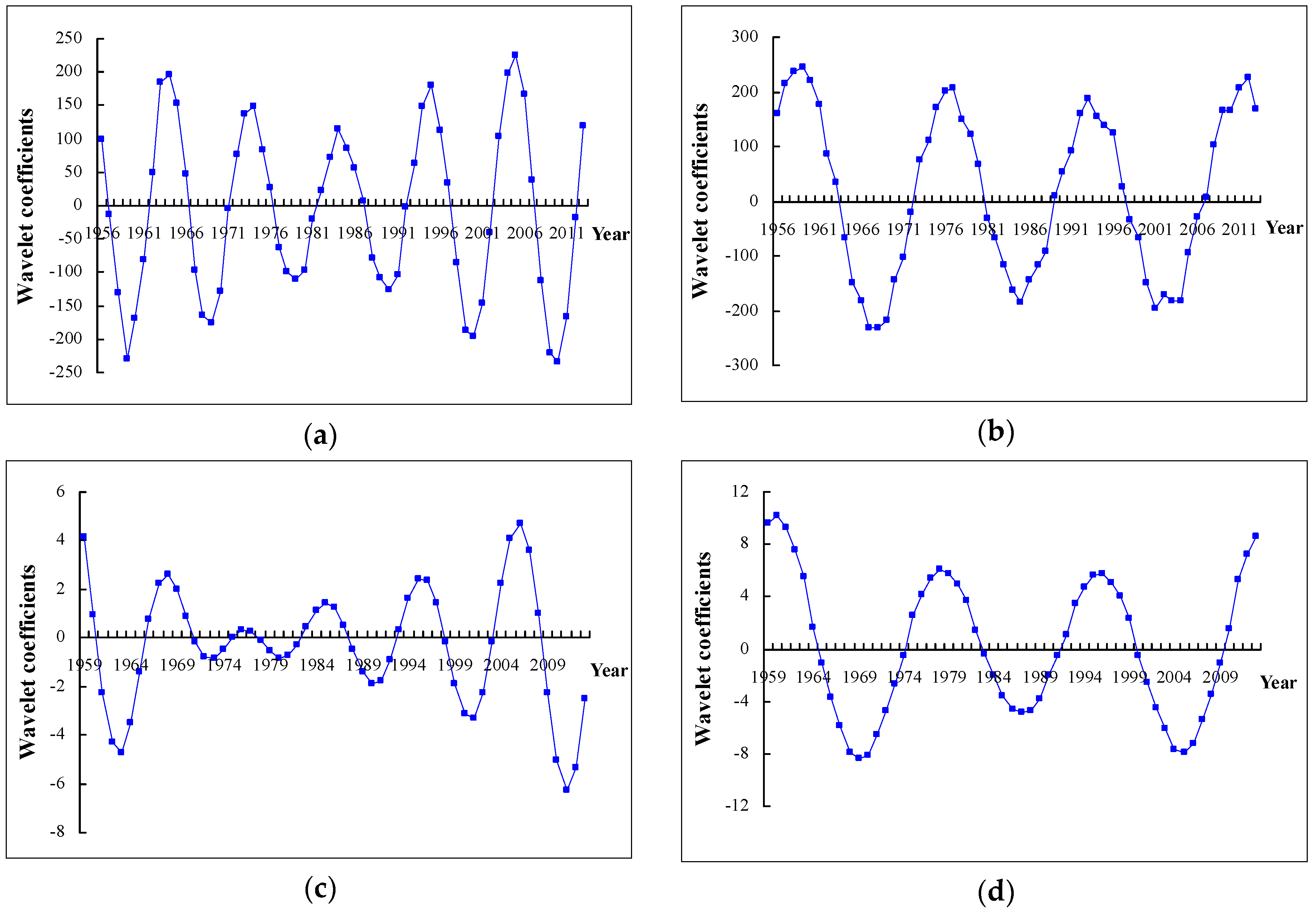
On the characteristic 15-year time-scale, the average period of annual precipitation change in the spring area was about 10 years and about 5 conversion periods (Figure 8a). On the 27-year characteristic time-scale (Figure 8b), the average period of precipitation was about 18 years, incorporating about 3 cycles of change in abundance. The characteristic 15-year time-scale for the spring water level had an average change period of 12 years (Figure 8c). The average period of spring water level change on the characteristic 27-year time-scale was about 16 years.
The results of continuous wavelet analysis show that the variation of atmospheric precipitation and spring water level has the same time-scale of 27 and 15 years, with typical periods for precipitation and spring water level being 16 and 12 years (Figure 7). Over long-term periods, atmospheric precipitation and spring water level showed an increasing trend. Wavelet analysis time-frequency characteristics in the local area can also be used to analyze the characteristics of atmospheric precipitation and spring water level changes at different scales over a long-term period [30]. The research results show that continuous wavelet transform can be used to characterize the temporal variability of the interrelationships involved, which is in good agreement with the research results of Jean [52].
3.3. Differences between the Trend of Atmospheric Precipitation and Spring Water Level Change
Normally, the level dynamic of the local groundwater shows significant multi-order autocorrelation, while the precipitation sequence does not show any autocorrelation and does not require pretreatment. Results for the calculation showed that the coefficient of variation of the sequence of groundwater level was 0.0627. As CV < 0.1, no pre-treatment was required. Results for the M-K mutation test were very similar to this result.
From 1959 to 2013, the groundwater level of Jinan spring dropped at a rate of 0.65 m/10a, and the average annual groundwater level U was less than 1.96, showing a significant (α = 0.05) decreasing trend. Average annual rainfall from 1956–2013 was 12.65 mm/10a (Table 1). Results for annual precipitation U were 0.2047 (<1.96), which did not pass the significance test of α = 0.05, thus the growth trend was deemed to not be significant.
Using the M-K trend analysis method, we obtained the trend of atmospheric precipitation and spring water level for the study period. Results showed that the trend of precipitation increase after 1999 was not significant, however the spring water level had a significant downward trend. This finding indicates that the decrease of precipitation was not the main cause for the decline in groundwater. Since 2003, remediation measures such as recharge and reducing groundwater exploitation in the spring field have resulted in an upward trend for the spring level, a trend response which is similar to that of atmospheric precipitation.
3.4. Atmospheric Rainfall and Detection of Spring Water Level Changes
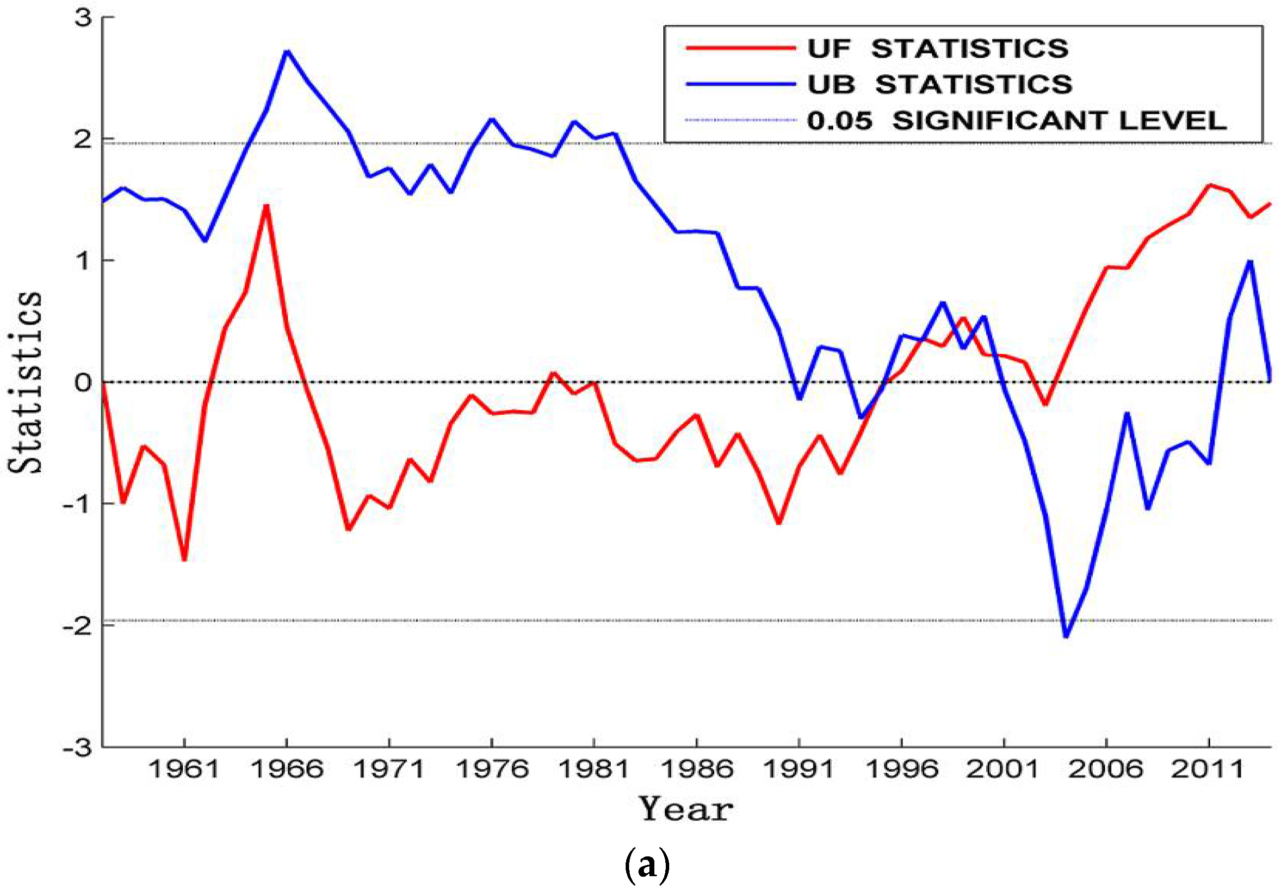
The M-K mutation test of annual average precipitation and average annual groundwater levels in the Jinan area showed that the fluctuation of atmospheric precipitation series UF was more complicated than the groundwater table (Figure 9a). UF results for precipitation from 1962–1967, a period of heavy precipitation, were greater than 0. UF in 1967 was equal to 0, and from 1967–1995, UF was less than 0. There is very little precipitation during this time. After 1996, only in 2002, the UF is less than 0. However, in the other remaining years the UF is greater than 0 and increases gradually. Moreover, the precipitation shows an increasing trend after 1996. Results for the UF and UB lines were found to intersect in 1999, and to be within the 2-letter reliability line, thus indicating a mutation at this time period. After 1999, precipitation increased.
From 1962–1966, the groundwater level of the spring group was higher than 0 (Figure 9b), this being the high water level of the groundwater level. However, this result did not pass the significance test of α = 0.05. UF results after 1967 were less than 0, indicating that the long-term underground water table was in a period of low water level. During this period the groundwater level was also recorded as declining. The only point of intersection between UF and UB occurred in 1967 and the intersection point was within 2 confidence lines of α = 0.05, indicating that an abrupt change of the water level occurred in 1967. The mean value of the groundwater level from 1959 to 1966 was 30.69 m, and after 1967 it was 27.25 m, thus showing significant differences. The UF was less than −1.96 after 1972, and the tendency of UF to continue to decrease before 2004 was obvious, indicating that the drop of groundwater level was significant. After 2004, the UF rapidly increased and the water level rapidly rose. The average water level after 2004 was 28.55 m.
Results from the M-K mutation test showed that the water level of the spring had a sudden change in 1967, and that the water level of the spring had a continuous decline after 1967 until 2004. A multiple regression model was established to examine the average water level during two different periods (1960–1967 and 1968–1989) and precipitation in the current year, urban exploitation, peripheral exploitation and precipitation in the previous year. The following equations were used:
where X1 is current precipitation; X2 is urban exploitation; X3 is external extraction; and X4 is precipitation of the previous year.
Y = 30.417 + 0.002X1 − 0.278X2 + 0.002X3 + 0.0004X4
Y = 27.362 + 0.002X1 − 0.002X2 − 0.05X3 + 0.001X4
Regression analysis results (Table 2) show that from the 1960s to the 1990s, the main factor affecting groundwater level changed from precipitation to artificial exploitation, and the influence of peripheral mining has exceeded that of urban mining. Under the conditions of mining, precipitation has become a secondary factor affecting the groundwater level in urban areas. Results from the regression analysis and the M-K mutation test method identified that mutation occurred for the spring level in 1967.
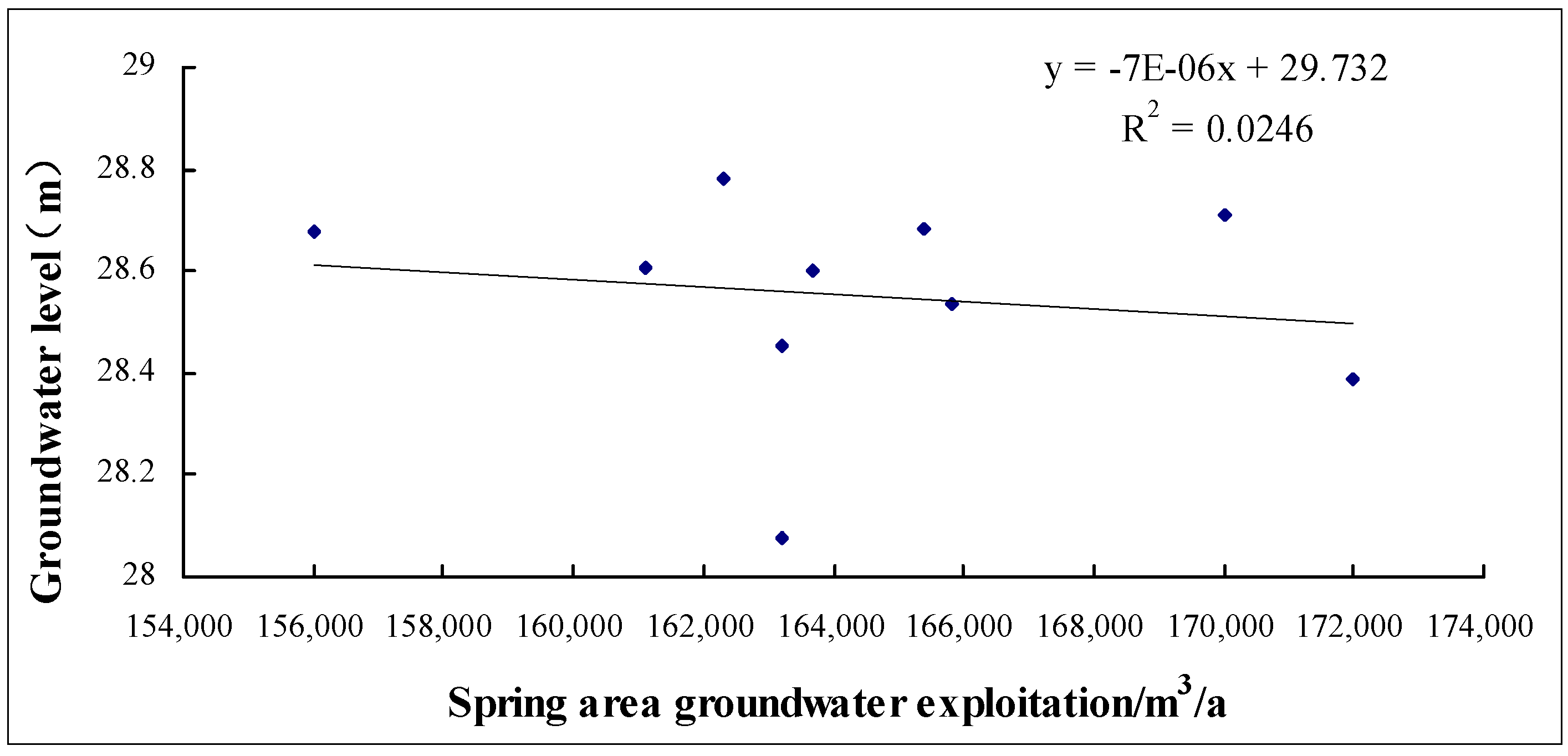
Before artificial recharge, a good correlation existed between the spring water level and extraction volume [53]. As the amount of extraction increased, the spring water level showed a downward trend (Figure 10). In order to restore the flowing state of the spring, the amount of groundwater exploitation was reduced and water recharge was undertaken in 2003. These remedial measures resulted in the correlation between spring water level and groundwater exploitation being significantly reduced (Figure 11). It can be presumed that if groundwater exploitation is small and stable, it can no longer be considered as the main factor affecting the spring water level changes. Zhang [47] also highlighted that the relationship between groundwater level and the amount of exploitation has not been significant since 1990.
M-K trend analysis can not only identify the significant trend of ascending and descending atmospheric precipitation and spring water series, it can also highlight the moment of mutation. However, the influencing factors of precipitation and water level are complex. Groundwater exploitation size, precipitation, rainfall station location and artificial recharge amount all have an impact on groundwater dynamics. Therefore, if M-K is used to analyze the characteristics of the catastrophe year and establish an appropriate prediction model, this will enable an improvement in accurately predicting future groundwater level changes. This is consistent with the results of Damir [54], which showed that the effects of spatial and temporal variations of hydrological time series and the space–time-variant behaviors of the karst system can be separated from the correlation functions.
4. Conclusions
Morlet wavelet transform for precipitation and groundwater table time series results in the Jinan spring area showing that there are numerous time-scales. The large time-scale includes the small time-scale, and the different time-scales imply different laws of change. Four time-scale periodic variation phases for atmospheric precipitation were identified (27, 15, 8 and 5-year) of which 27 and 15 years corresponded to the variation period of 16 and 12 years. Results for the spring water level also recorded 27- and 15-year time-scales, with a period of change of 16 and 12 years. Average annual increase in precipitation from 1956 to 2013 was 12.65 mm/10a, results indicating there was no significant increase. The rate of decline of the groundwater level from 1959 to 2013 was 0.65 m/10a, recording a significant downward trend. After a sudden change in 1999, precipitation increased thereafter. 1967 was identified as the year sudden water level changes occurred at the spring, which was noted by a significant reduction in the water level. By establishing a multiple regression model for different periods, the main factors influencing groundwater levels in Jinan over the last 50 years included atmospheric precipitation and artificial extraction. After remediation measures were implemented, such as recharge and limiting groundwater exploitation in 2003, the future trend of water level should be in line with the precipitation, and have an upward trend.
Results from our investigation have shown that the wavelet analysis method and the M-K method have their own strengths. The results of the two methods were mutually verified and were found to complement each other. These methods are feasible for identifying the dynamic variation of groundwater in a heterogeneous karst aquifer system. The groundwater level not only relates to the amount of groundwater resources, but also relates to many geological and ecological problems. The unreasonable development and utilization of groundwater resources will lead to a series of geological environmental problems, such as land subsidence, ground fissures, and seawater intrusion. At the same time, groundwater level is also the key to prevent soil salinization and maintain the ecological environment in arid areas. Therefore, the study of the difference in the delay of precipitation response to groundwater level can help improve the prediction and warning model of groundwater level and improve the work accuracy. Although this study has reached certain conclusions, there are still some problems, such as the incompleteness of data. If we use numerical simulation and field in-situ experiments in future studies, we can better manage karst springs.
Author Contributions
L.X. and G.C. conceived and designed the experiments; L.H. performed the experiments; L.Y. and C.L. analyzed the data; X.H. contributed reagents/materials/analysis tools; L.X. and G.C. wrote the paper.
Acknowledgments
This research is supported by the National Natural Science Foundation of China (41772257, 41472216), the Project of Shandong Province Higher Educational Science and Technology Program (J17KA191).
Conflicts of Interest
The authors declare no conflict of interest. The founding sponsors had no role in the design of the study; in the collection, analyses, or interpretation of data; in the writing of the manuscript, and in the decision to publish the results.
References
- Guo, L.; Gong, H.L.; Zhu, F.; Guo, X.M.; Zhou, C.F.; Qiu, L. Cyclical characteristics of groundwater level and precipitation based on wavelet analysis. Geogr. Geo-Inf. Sci. 2014, 30, 35–38. [Google Scholar]
- Nakken, M. Wavelet analysis of rainfall–runoff variability isolating climatic from anthropogenic patterns. Environ. Model. Softw. 1999, 14, 283–295. [Google Scholar] [CrossRef]
- Qi, X.; Yang, L.; Han, Y.; Shang, H.; Xing, L. Cross wavelet analysis of groundwater level regimes and precipitation-groundwater level regime in Ji’nan spring region. Adv. Earth Sci. 2012, 27, 969–978. [Google Scholar]
- Tremblay, L.; Larocque, M.; Anctil, F.; Rivard, C. Teleconnections and interannual variability in Canadian groundwater levels. J. Hydrol. 2011, 410, 178–188. [Google Scholar] [CrossRef]
- Xiao-Fan, Q.I.; Jiang, Z.C.; Luo, W.Q. Cross wavelet analysis of relationship between precipitation and spring discharge of a typical epikarst water system. Earth Environ. 2012, 40, 561–567. [Google Scholar]
- Chi, G.Y.; Xing, L.T.; Zhu, H.X.; Hou, X.Y.; Xiang, H.; Xing, X.R. The study of quantitative relationship between the spring water and the dynamic change of the atmospheric precipitation in Ji’nan. Ground Water 2017, 39, 8–11. [Google Scholar]
- Li, X.; Li, G.; Zhang, Y. Identifying major factors affecting groundwater change in the north China plain with grey relational analysis. Water 2014, 6, 1581–1600. [Google Scholar] [CrossRef]
- Chang, F.J.; Chen, P.A.; Liu, C.W.; Liao, H.C.; Liao, C.M. Regional estimation of groundwater arsenic concentrations through systematical dynamic-neural modeling. J. Hydrol. 2013, 499, 265–274. [Google Scholar] [CrossRef]
- Jan, C.D.; Chen, T.H.; Huang, H.M. Analysis of rainfall-induced quick groundwater-level response by using a kernel function. Paddy Water Environ. 2013, 11, 135–144. [Google Scholar] [CrossRef]
- Ke-Zhen, H.U.; Zhang, J.Z.; Xing, L.T. Study on dynamic characteristics of groundwater based on the time series analysis method. Water Sci. Eng. Technol. 2011, 5, 32–34. [Google Scholar]
- Lu, W.X.; Zhao, Y.; Chu, H.B.; Yang, L.L. The analysis of groundwater levels influenced by dual factors in western Jilin province by using time series analysis method. Appl. Water Sci. 2014, 4, 251–260. [Google Scholar] [CrossRef]
- Zhou, T.; Wang, F.; Yang, Z. Comparative analysis of ANN and SVM models combined with wavelet preprocess for groundwater depth prediction. Water 2017, 9, 781. [Google Scholar] [CrossRef]
- Arenas, A.; Schilling, K.; Niemeier, J.; Weber, L. Evaluating the timing and interdependence of hydrologic processes at the watershed scale based on continuously monitored data. Water 2018, 10, 261. [Google Scholar] [CrossRef]
- Huang, L.; Wang, L.; Zhang, Y.; Xing, L.; Hao, Q.; Xiao, Y.; Yang, L.; Zhu, H. Identification of groundwater pollution sources by a SCE-UA algorithm-based simulation/optimization model. Water 2018, 10, 193. [Google Scholar] [CrossRef]
- Faulkner, J.; Hu, B.X.; Kish, S.; Hua, F. Laboratory analog and numerical study of groundwater flow and solute transport in a karst aquifer with conduit and matrix domains. J. Contam. Hydrol. 2009, 110, 34–44. [Google Scholar] [CrossRef] [PubMed]
- Sun, C.; Shu, L.C.; Lu, C.P.; Zhang, C.Y. Physical experiment and numerical simulation of spring flow attenuation process in fissure-conduit media. J. Hydraul. Eng. 2014, 45, 50–57. [Google Scholar]
- Gallegos, J.J. Modeling Groundwater Flow in Karst Aquifers: An Evaluation of Modflow-CFP at the Laboratory and Sub-Regional Scales; Florida State University: Tallahassee, FL, USA, 2011. [Google Scholar]
- Gong, H.L.; Zhao, W.J.; Zhu, Y.Q. Numerical emulation of fissure-karst water and optimization of seepage field. Acta Simul. Syst. Sin. 2002, 14, 186–188. [Google Scholar]
- Shoemaker, W.B.; Kuniansky, E.L.; Birk, S.; Bauer, S.; Swain, E.D. Documentation of a conduit flow process (CFP) for modflow-2005. In Techniques & Methods; U.S. Geological Survey: Reston, VA, USA, 2005; pp. 1–50. [Google Scholar]
- Taweesin, K.; Seeboonruang, U.; Saraphirom, P. The influence of climate variability effects on groundwater time series in the lower central plains of Thailand. Water 2018, 10, 290. [Google Scholar] [CrossRef]
- Dvory, N.Z.; Livshitz, Y.; Kuznetsov, M.; Adar, E.; Yakirevich, A. The effect of hydrogeological conditions on variability and dynamic of groundwater recharge in a carbonate aquifer at local scale. J. Hydrol. 2015, 535, 480–494. [Google Scholar] [CrossRef]
- Thomas, B.F.; Behrangi, A.; Famiglietti, J.S. Precipitation intensity effects on groundwater recharge in the southwestern United States. Water 2016, 8, 90. [Google Scholar] [CrossRef]
- Xiaofan, Q.I.; Wenpeng, L.I.; Chuansheng, L.I.; Yang, L.; Yuhong, M.A. Trends and persistence of groundwater table and precipitation of Ji’nan karst springs watershed. J. Irrig. Drain. 2015, 34, 98–104. [Google Scholar]
- Wu, X.L.; Zhang, B.; Ai, N.S.; Liu, L.J. Wavelet analysis on SO2 pollution index changes of Shanghai in recent 10 years. Environ. Sci. 2009, 30, 2193–2198. [Google Scholar]
- Echer, M.P.S.; Echer, E.; Nordemann, D.J.; Rigozo, N.R.; Prestes, A. Wavelet analysis of a centennial (1895–1994) Southern Brazil Rainfall series (Pelotas, 31°46′19″ S 52°20′ 33″ W). Clim. Chang. 2008, 87, 489–497. [Google Scholar] [CrossRef]
- Jongh, I.L.M.D.; Verhoest, N.E.C.; Troch, F.P.D. Analysis of a 105-year time series of precipitation observed at Uccle, Belgium. Int. J. Climatol. 2006, 26, 2023–2039. [Google Scholar] [CrossRef]
- Kahya, E.; Kalaycı, S. Trend analysis of streamflow in turkey. J. Hydrol. 2004, 289, 128–144. [Google Scholar] [CrossRef]
- Rascher, E.; Sass, O. Evaluating sediment dynamics in tributary trenches in an alpine catchment (Johnsbachtal, Austria) using multi-temporal terrestrial laser scanning. Z. Geomorphol. Suppl. 2017, 61, 27–52. [Google Scholar] [CrossRef]
- Groisman, P.Y.; Knight, R.W.; Karl, T.R. Changes in intense precipitation over the Central United States. J. Hydrometeorol. 2012, 13, 47–66. [Google Scholar] [CrossRef]
- Rajah, K.; O’Leary, T.; Turner, A.; Petrakis, G.; Leonard, M.; Westra, S. Changes to the temporal distribution of daily precipitation. Geophys. Res. Lett. 2015, 41, 8887–8894. [Google Scholar] [CrossRef]
- Fujibe, F. The increasing trend of intense precipitation in Japan based on four-hourly data for a hundred years. Sola 2005, 1, 41–44. [Google Scholar] [CrossRef]
- Kamruzzaman, M. Peer review report 2 on statistical analysis of sub-daily precipitation extremes in singapore. J. Hydrol. Reg. Stud. 2015, 3, 3–4. [Google Scholar] [CrossRef]
- Trenberth, K.E. Changes in precipitation with climate change. Clim. Res. 2011, 47, 123–138. [Google Scholar] [CrossRef]
- Seghieri, J.; Vescovo, A.; Padel, K.; Soubie, R.; Arjounin, M.; Boulain, N.; Rosnay, P.D.; Galle, S.; Gosset, M.; Mouctar, A.H. Relationships between climate, soil moisture and phenology of the woody cover in two sites located along the west African latitudinal gradient. J. Hydrol. 2009, 375, 78–89. [Google Scholar] [CrossRef]
- Belle, G.V.; Hughes, J.P. Nonparametric tests for trend in water quality. Water Resour. Res. 1984, 20, 127–136. [Google Scholar] [CrossRef]
- Hamed, K.H. Exact distribution of the Mann-Kendall trend test statistic for persistent data. J. Hydrol. 2009, 365, 86–94. [Google Scholar] [CrossRef]
- Jiang, X.; Liu, S.; Ma, M.; Zhang, J. A wavelet analysis of the temperature time series in northeast China during the last 100 years. Adv. Clim. Chang. Res. 2008, 27, 122–128. [Google Scholar]
- Sang, Y.F.; Dong, W. Wavelets selection method in hydrologic series wavelet analysis. J. Hydraul. Eng. 2008, 39, 295–300. [Google Scholar]
- Shen, Q.Q.; Shu, J.; Wang, X.H. Multiple time scales analysis of temperature and precipitation variation in shanghai for the recent 136 years. J. Nat. Resour. 2011, 26, 644–654. [Google Scholar]
- Tirogo, J.; Jost, A.; Biaou, A.; Valdes-Lao, D.; Koussoubé, Y.; Ribstein, P. Climate variability and groundwater response: A case study in Burkina Faso (west Africa). Water 2016, 8, 171. [Google Scholar] [CrossRef]
- Chiaudani, A.; Curzio, D.D.; Palmucci, W.; Pasculli, A.; Polemio, M.; Rusi, S. Statistical and fractal approaches on long time-series to surface-water/groundwater relationship assessment: A central Italy alluvial plain case study. Water 2017, 9, 850. [Google Scholar] [CrossRef]
- Liu, Y.L.; Zhai, X.L.; Zheng, A.Q. Analysis of precipitation trend in the Guanzhong basin based on the Mann-Kendall method. Yellow River 2012, 34, 28–30. [Google Scholar]
- Qi, X.F.; Wang, Y.S.; Yang, L.Z.; Liu, Z.Y.; Wang, W.; Wen-Peng, L.I. Time lags variance of groundwater level response to precipitation of Ji’nan karst spring watershed in recent 50 years. Carsol. Sin. 2016, 35, 384–393. [Google Scholar]
- Yu, Y.S.; Chen, X.W. Study on the percentage of trend component in a hydrological time series based on Mann-Kendall method. J. Nat. Resour. 2011, 26, 1585–1591. [Google Scholar]
- Zhang, Q.; Xu, C.Y.; Tao, H.; Jiang, T.; Chen, Y.D. Climate changes and their impacts on water resources in the arid regions: A case study of the Tarim river basin, China. Stoch. Environ. Res. Risk Assess. 2010, 24, 349–358. [Google Scholar] [CrossRef]
- Wang, J.; Jin, M.; Wang, J.; Jin, M. Hydrochemical characteristics and formation causes of karst water in jinan spring catchment. Diqiu Kexue Zhongguo Dizhi Daxue Xuebao/Earth Sci. J. China Univ. Geosci. 2017, 42, 821–831. [Google Scholar]
- Zhang, J.Z.; Yan, L.T. Application of regression analysis in the groundwater dynamic analysis. Ground Water 2010, 32, 88–90. [Google Scholar]
- Labat, D. Cross wavelet analyses of annual continental freshwater discharge and selected climate indices. J. Hydrol. 2010, 385, 269–278. [Google Scholar] [CrossRef]
- Labat, D.; Ababou, R.; Mangin, A. Rainfall-runoff relations for karstic springs. Part II: Continuous wavelet and discrete orthogonal multiresolution analyses. J. Hydrol. 2000, 238, 149–178. [Google Scholar] [CrossRef]
- Labat, D.; Ronchail, J.; Guyot, J.L. Recent advances in wavelet analyses: Part 2—Amazon, Parana, Orinoco and Congo discharges time scale variability. J. Hydrol. 2005, 314, 289–311. [Google Scholar] [CrossRef]
- Mann, H.B. Nonparametric test against trend. Econometrica 1945, 13, 245–259. [Google Scholar] [CrossRef]
- Charlier, J.B.; Ladouche, B.; Maréchal, J.C. Identifying the impact of climate and anthropic pressures on karst aquifers using wavelet analysis. J. Hydrol. 2015, 523, 610–623. [Google Scholar] [CrossRef]
- Zhou, J.; Xing, L.T.; Teng, Z.X.; Wang, L.Y. Study on the Threshold of Main Factors Restricting Ji’nan Large Karst Springs Spewing; East China Normal University: Shanghai, China, 2015; pp. 146–156. [Google Scholar]
- Jukić, D.; Denić-Jukić, V. Investigating relationships between rainfall and karst-spring discharge by higher-order partial correlation functions. J. Hydrol. 2015, 530, 24–36. [Google Scholar] [CrossRef]
Figure 1.
Hydrographic map of the Jinan spring area.

Figure 2.
Geological profile schematic diagram.

Figure 3.
Precipitation and spring water level contrast curve, 1959 to 2013.
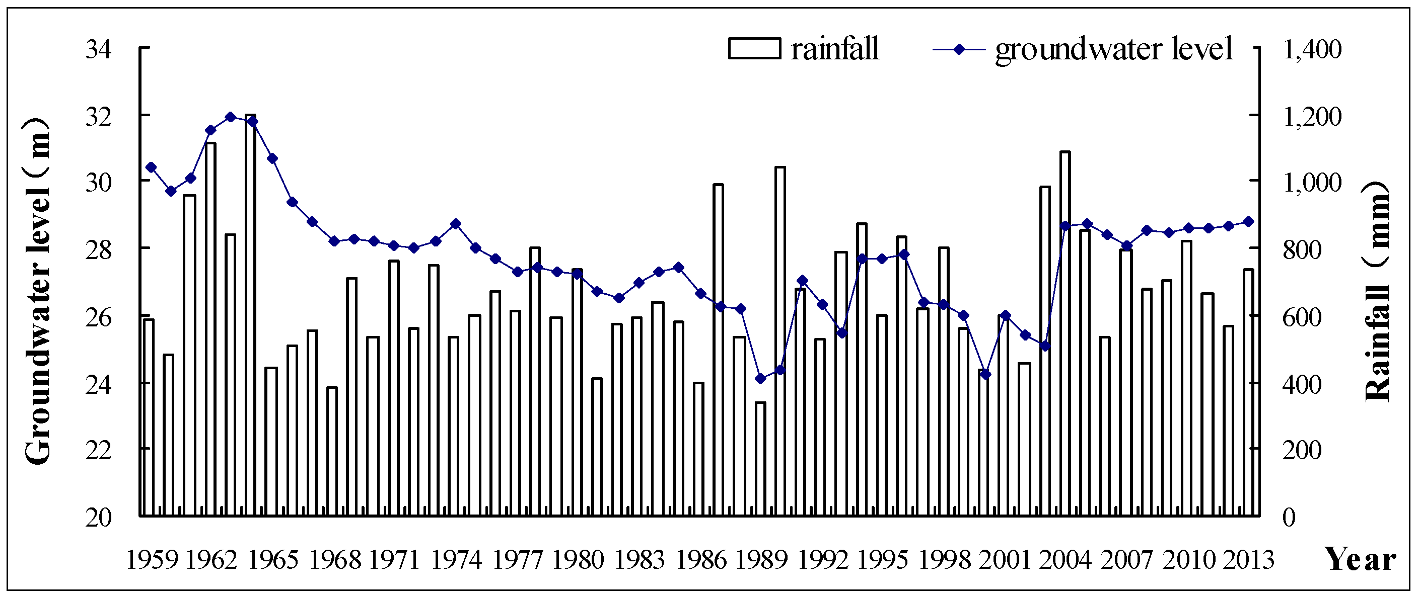
Figure 4.
Wavelet coefficient contour map. (a) For atmospheric precipitation; (b) for spring water level.
Figure 4.
Wavelet coefficient contour map. (a) For atmospheric precipitation; (b) for spring water level.

Figure 5.
Wavelet coefficient model contour map. (a) For atmospheric precipitation; (b) for spring water level.
Figure 5.
Wavelet coefficient model contour map. (a) For atmospheric precipitation; (b) for spring water level.
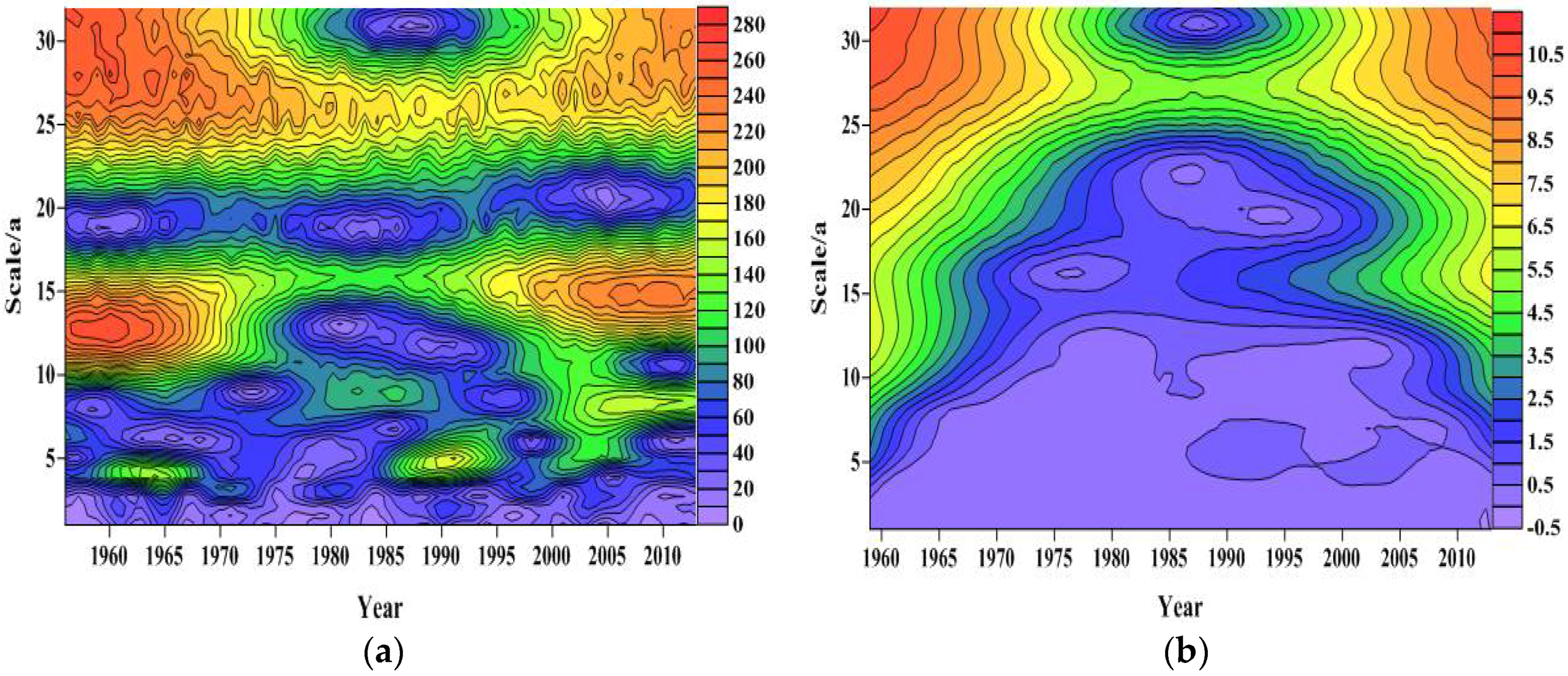
Figure 6.
Contour map of the wavelet coefficients modulus square. (a) For atmospheric precipitation; (b) for spring water level.
Figure 6.
Contour map of the wavelet coefficients modulus square. (a) For atmospheric precipitation; (b) for spring water level.

Figure 7.
Wavelet variance plot. (a) For atmospheric precipitation; (b) for spring water level.

Figure 8.
Wavelet coefficient main period chart. (a) 15-year scale for atmospheric precipitation; (b) 27-year scale for atmospheric precipitation; (c) 15-year scale for spring water level; (d) 27-year scale for spring water level.
Figure 8.
Wavelet coefficient main period chart. (a) 15-year scale for atmospheric precipitation; (b) 27-year scale for atmospheric precipitation; (c) 15-year scale for spring water level; (d) 27-year scale for spring water level.

Figure 9.
M-K mutation test chart. (a) For atmospheric precipitation; (b) for spring water level.

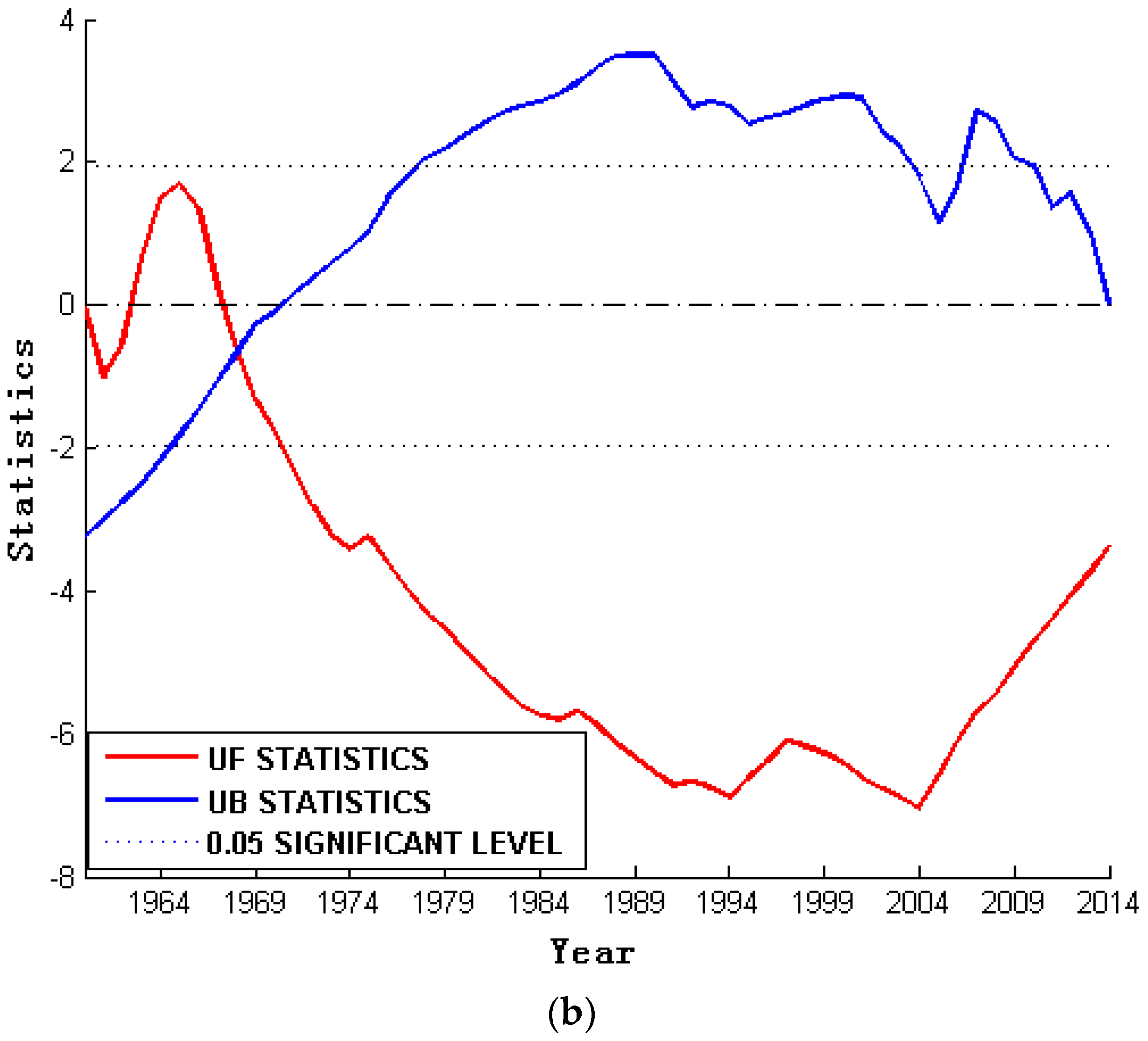
Figure 10.
Relationship between spring water level and exploitation volume, 1959–1989.
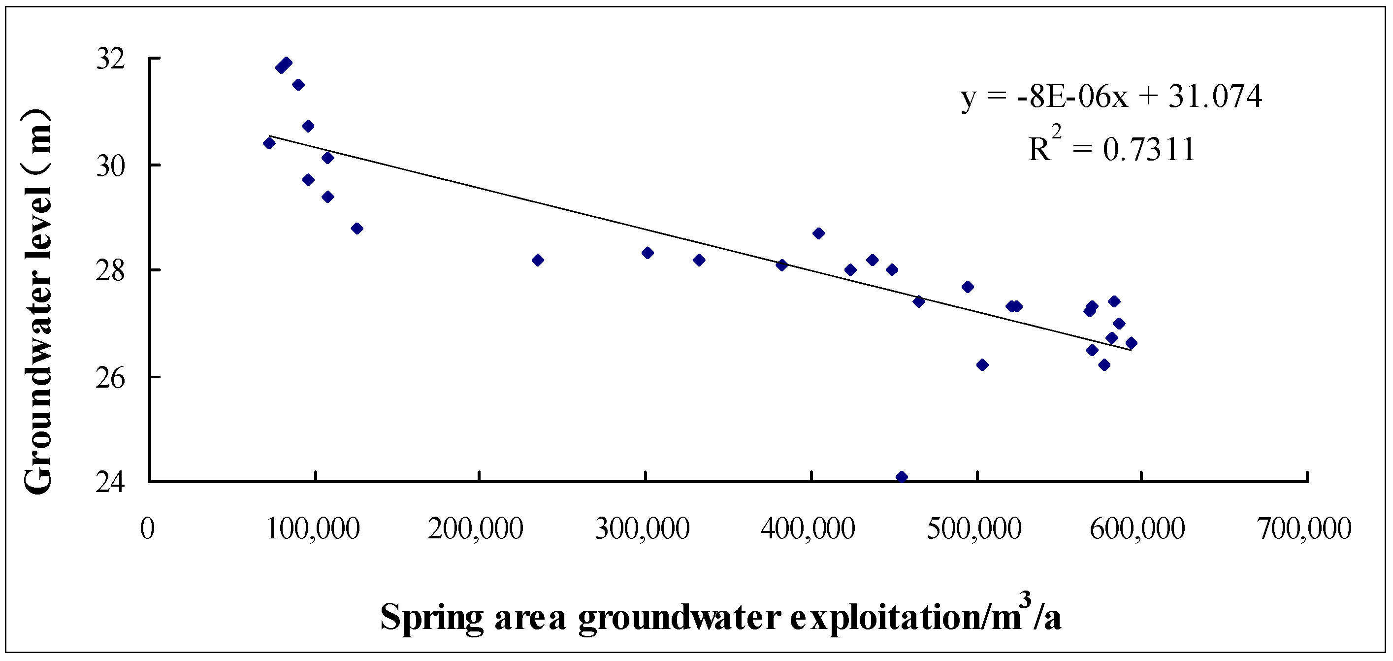
Figure 11.
Relationship between groundwater exploitation and spring water level, 2003–2012.

Table 1.
M-K trend test results list.
| Project | U | β |
|---|---|---|
| Annual groundwater level | 0.9996 | −0.065 |
| Annual precipitation | 0.2047 | 1.2647 |
Table 2.
Partial correlation coefficients between various factors and groundwater levels.
| Influencing Factors | Year | |
|---|---|---|
| 1960–1967 | 1968–1989 | |
| Current precipitation and groundwater level | 0.959 | 0.285 |
| Precipitation and groundwater level in the previous year | 0.95 | 0.094 |
| The first two years of precipitation and groundwater level | 0.479 | |
| Urban exploitation and groundwater level | −0.873 | −0.017 |
| Periphery exploitation and groundwater level | −0.572 | |
© 2018 by the authors. Licensee MDPI, Basel, Switzerland. This article is an open access article distributed under the terms and conditions of the Creative Commons Attribution (CC BY) license (http://creativecommons.org/licenses/by/4.0/).
Share and Cite
MDPI and ACS Style
Xing, L.; Huang, L.; Chi, G.; Yang, L.; Li, C.; Hou, X. A Dynamic Study of a Karst Spring Based on Wavelet Analysis and the Mann-Kendall Trend Test. Water 2018, 10, 698. https://doi.org/10.3390/w10060698
AMA Style
Xing L, Huang L, Chi G, Yang L, Li C, Hou X. A Dynamic Study of a Karst Spring Based on Wavelet Analysis and the Mann-Kendall Trend Test. Water. 2018; 10(6):698. https://doi.org/10.3390/w10060698
Chicago/Turabian StyleXing, Liting, Linxian Huang, Guangyao Chi, Lizhi Yang, Changsuo Li, and Xinyu Hou. 2018. "A Dynamic Study of a Karst Spring Based on Wavelet Analysis and the Mann-Kendall Trend Test" Water 10, no. 6: 698. https://doi.org/10.3390/w10060698
Note that from the first issue of 2016, this journal uses article numbers instead of page numbers. See further details here.