Subpixel Surface Water Extraction (SSWE) Using Landsat 8 OLI Data
by
 , ,
, ,
Longhai Xiong
1, 
Ruru Deng
1,*,
Jun Li
1, 
Xulong Liu
2,
Yan Qin
1,
Yeheng Liang
1 and
Yingfei Liu
1 1
Guangdong Engineering Research Center of Water Environment Remote Sensing Monitoring, Guangdong Provincial Key Laboratory of Urbanization and Geo-simulation, School of Geography and Planning, Sun Yat-sen University, Guangzhou 510275, China
2
Key Laboratory of Guangdong for Utilization of Remote Sensing and Geographical Information System, Guangzhou Institute of Geography, Guangzhou 510070, China
*
Author to whom correspondence should be addressed.
Water 2018, 10(5), 653; https://doi.org/10.3390/w10050653
Submission received: 22 March 2018
/
Revised: 14 May 2018
/
Accepted: 15 May 2018
/
Published: 18 May 2018
(This article belongs to the Section Water Resources Management, Policy and Governance)
Abstract
:Surface water extraction from remote sensing imagery has been a very active research topic in recent years, as this problem is essential for monitoring the environment, ecosystems, climate, and so on. In order to extract surface water accurately, we developed a new subpixel surface water extraction (SSWE) method, which includes three steps. Firstly, a new all bands water index (ABWI) was developed for pure water pixel extraction. Secondly, the mixed water–land pixels were extracted by a morphological dilation operation. Thirdly, the water fractions within the mixed water–land pixels were estimated by local multiple endmember spectral mixture analysis (MESMA). The proposed ABWI and SSWE have been evaluated by using three data sets collected by the Landsat 8 Operational Land Imager (OLI). Results show that the accuracy of ABWI is higher than that of the normalized difference water index (NDWI). According to the obtained surface water maps, the proposed SSWE shows better performance than the automated subpixel water mapping method (ASWM). Specifically, the root-mean-square error (RMSE) obtained by our SSWE for the data sets considered in experiments is 0.117, which is better than that obtained by ASWM (0.143). In conclusion, the SSWE can be used to extract surface water with high accuracy, especially in areas with optically complex aquatic environments.
1. Introduction
Surface water provides water resources for various human uses [1] and is critical to floral and faunal habitat [2]. With the ever-increasing human population and accelerated social development, persistent stress is exerted on surface water resources [3], as surface water is essential for many applications, such as sustained water resource management [4,5,6,7]. However, conventional in situ measurements of the extent of surface water are limited in terms of spatial coverage and frequency [8].
In the past years, remote sensing has been an efficient technique for the extraction of surface water. It can provide data at various temporal scales, with large spatial coverage, low cost, among other benefits. Specifically, many satellite sensors with different spatial, temporal, and spectral resolution have been applied for the extraction of surface water, such as the Moderate-Resolution Imaging Spectroradiometer (MODIS) [9,10], Worldview [11], Satellite Pour l’Observation de la Terre (SPOT) [12], Advanced Spaceborne Thermal Emission and Reflection Radiometer (ASTER) [13], Advanced Very High Resolution Radiometer (AVHRR) [14], Landsat [15,16], HJ-1A/B [17], ZY-3 [18], and others. Among these sensors, those with high temporal resolution are generally limited in terms of spatial resolution, while those with high spatial resolution are mostly limited in terms of revisit time and cost [16]. Due to its good tradeoff in terms of spatial and temporal resolution, cost-free access, and continuity over 40 years, Landsat has become one of the most widely used optical sensors for surface water research. Particularly, significant improvements in signal-to-noise ratio and radiometric resolution make the Landsat-8 Operational Land Imager (OLI) a very promising instrument for enhanced extraction and monitoring of optically complex surface water [19].
Commonly adopted surface water extraction methods based on optical images include digitizing through visual interpretation, single-band thresholding [15,20,21], multiple-band spectral water indices [10,18,22,23,24], image processing methods [25,26], and target detection methods, such as constrained energy minimization (CEM) [27]. Each of these methods exhibits advantages and limitations. Combinations of the above methods have been also proposed to improve water extraction performance [16,27,28,29,30,31,32,33]. Among these water extraction methods, multiple-band spectral water indices are the most popular ones due to their simplicity, cost-effectiveness, and reproducibility [10].
Although there are many water extraction methods available in the literature, most of them extract surface water just at the pixel level. This means that these methods ultimately classify each pixel as water or non-water. However, real scenes are dominated by mixed pixels (particularly, there are many water–land mixing interactions in estuaries, braid rivers, marsh, mulberry fish ponds, etc.), which often cause classification uncertainty. Furthermore, the limited spatial resolution of satellite images (e.g., 30 m in the case of OLI) generally leads to a predominance of pixels that are mixed by several land cover classes, which appear at scales that are smaller than the pixel resolution [34]. Therefore, most of the aforementioned methods are unable to correctly identify the proportions of water in mixed pixels, which results in an insufficient accuracy of surface water extraction. Since water extent variations are critical to many applications, such as estimating the spatiotemporal water body changes, the errors caused by the presence of mixed pixels should be addressed properly for accurate surface water extent extraction [16].
Several subpixel processing methods have been used to address the problem of spectral mixture of water and land. Among them are soft classification techniques [16,35], machine learning models (such as random forest regression model and regression tree) [36,37,38], and spectral mixture analysis (SMA) [39,40,41,42]. The soft classification techniques do not estimate the water fraction directly, but instead provide an estimate of class membership, which is commonly used to convert mixed pixels into water or non-water through a threshold value [16,35]. The machine learning methods commonly require training data from field measurements or high-resolution images. SMA is a physically based technique which can be used to estimate the percent cover of surface water without the need for extensive training data. To derive subpixel water fraction, Xie et al. [42] developed an automated subpixel water mapping method (ASWM), based on a water index (normalized difference water index, NDWI) and a linear spectral mixture analysis (LSMA) model. Halabisky et al. [39] used spectral mixture analysis (SMA) of Landsat satellite imagery to reconstruct surface water hydrographs.
Deficiencies are present in the above subpixel water extraction methods using SMA: (1) Only a few bands are considered in pure water pixel extraction with previous water indices methods, which could lead to information loss for other bands. A method taking advantage of all bands in remote sensors is assumed to be more effective in water extraction. (2) It is difficult to solve the issue of strong spectral variability in the water class using the conventional LSMA. Multiple endmember spectral mixture analysis (MESMA), which allows the number and type of endmembers to vary on a per-pixel basis [43], can address this limitation, offering competitive performance for subpixel mapping of land cover [44,45,46,47].
Consequently, in order to tackle the aforementioned problems, in this study, we developed a new subpixel surface water extraction (SSWE) method, which includes: (1) developing a new water index (ABWI) to extract pure water pixels by fully utilizing all the bands information; (2) extracting the mixed water–land pixels by a morphological dilation operation; and (3) developing a local MESMA approach to dynamically extract multiple water endmembers and identify the water fractions in mixed water–land pixels.
The remainder of this work is organized as follows. Section 2 introduces three test sites (and their reference maps) that have been considered for test and validation purposes. Section 3 introduces the proposed SSWE method, as well as the adopted accuracy metrics. Section 4 presents the results obtained by the proposed ABWI and SSWE in the task of surface water extraction. Comparisons with other methods are also included in this section. Section 5 discusses the results and hints at plausible future research lines. Finally, Section 6 concludes the paper, with some remarks.
2. Materials
2.1. Test Sites
The three test sites considered in experiments are located in Guangdong Province, China. They comprise different surface water types, landscapes, and mixed water pixels, including rivers, reservoirs, and estuaries that differ in turbidity, depth, and the level of water pollution. These sites were deliberately selected so that the subscenes contain water bodies with diverse spectra. Figure 1 illustrates the location of the three test sites and their false color images. The first data set (Figure 1b) is the Dongjiang River, which is a complex aquatic environment under an urban background, polluted by domestic sewage and waste water from manufactories. The second data set (Figure 1c) is the Dongbao Estuary, which contains diverse water bodies, including turbid rivers with urban surfaces, shallow mulberry fish ponds, tidal creeks, and the ocean. The last test site (Figure 1d) is the Tiegang Reservoir, characterized by the presence of clear water with many branches. Water–land mixed pixels exist in all these test sites, among which the number of water–land mixed pixels in Dongbao Estuary is the most significant, owing to the presence of many mulberry fish ponds.
2.2. Landsat 8 OLI Data
For the three considered test sites, orthorectified and terrain-corrected Landsat 8 OLI images in GeoTIFF format were obtained from the United States Geological Survey (USGS) EarthExplorer [48], all of them of product type Level 1 T. All Landsat 8 OLI images were defined in Universal Transverse Mercator (UTM) map projection and georeferenced with a precision better than 0.4 pixels [49]. Additional details, including the acquisition date, cloud cover, and scene ID of the OLI images are given in Table 1. All Landsat images were clipped to 230 × 230 pixels because the sizes of Landsat images were much larger than that of the reference data. All subsets were cloud-free to decrease the influence of clouds on the data. These images, acquired on specific dates, were selected because high-resolution images acquired on the same dates for reference can be found in Google Earth™. The acquisition dates of all the Landsat 8 OLI images were in the dry season. On the acquisition dates of the images used for the three test sites, days from the last rainfall event were 6, 4, and 6, respectively. The Landsat 8 OLI image at Dongbao Estuary was acquired during low tide.
2.3. Reference Data
For the three test sites, the fine spatial resolution Google Earth™ images (<1 m) were used for reference. The acquisition dates of the reference data and the Landsat 8 OLI images were exactly the same. From Google Earth, we can obtain the acquisition dates of the Google Earth™ images, however, the acquisition time of these images were unavailable. The short time span between the Google Earth™ images and the Landsat 8 OLI images was inevitable. Generally, the surface water boundaries change little during a short time period, though the tide may influence surface water extent at Dongbao Estuary, where the changes in water level were less than 0.4 m from 9 a.m. to 12 p.m. on the image acquisition date. The Landsat 8 OLI images were registered to the Google Earth™ images using a first-order polynomial with 10 ground control points (GCPs) manually selected from each image in ENVI v.5.3 [50]. The GCPs were located mainly at road junctions, and the corresponding root-mean-square error (RMSE) values for the three test sites were 0.21, 0.26, and 0.28 pixels, respectively. The “true” boundaries of surface water bodies were obtained via manual digitization on-screen from the reference data. Then, the “true” surface waterbody maps were overlaid on the 30 m grids of the Landsat data to generate the “true” water fraction images at the 30 m resolution, which were used to assess the accuracy of the different water extraction methods considered in this work.
3. Methods
3.1. Image Preprocessing
The raw Landsat 8 OLI images are in the form of digital numbers (DNs), which often need to be converted into apparent surface reflectance before processing. In this work, radiometric calibration and atmospheric correction were applied to all used images. Radiometric calibration converted the original DNs into top of atmosphere (TOA) radiances [W/(m2·sr·μm)]. For a given wavelength λ, the TOA radiance was derived from the following equation:
where is the gain factor and is the offset, which were provided in the Level 1 Product Generation System (LPGS) metadata file. Atmospheric correction was applied to the radiometrically calibrated images using the Fast Line-of-Sight Atmospheric Analysis of Spectral Hypercubes (FLAASH) module in ENVI v.5.3 [50]. The atmospheric parameters were obtained from a look-up table based on a seasonal-latitude surface temperature module [51]. Aerosol optical depth (AOD) data was obtained from the Level 2.0 AERONET data [52]. Though many approaches existed to correct for atmospheric effects with high accuracy, FLAASH was selected because it was commonly used in many recent surface water extraction researches based on Landsat 8 OLI data [16,42].
3.2. Subpixel Surface Water Extraction
The subpixel surface water extraction (SSWE) method includes three major steps. Firstly, an all bands water index (ABWI) was developed to classify the pure water and land classes. In this step, the water–land mixed pixels were classified as land. Secondly, we used a morphological dilation operation to identify the mixed water–land pixels. Thirdly, a local MESMA procedure was developed for unmixing the mixed pixels. The details of the SSWE are given below.
3.2.1. Extraction of Pure Water Pixels
Previous studies have revealed the spectral signatures of major land cover types [22,53]. It was found that the water shows higher reflectance of visible bands than infrared bands in most cases. Few non-water surface possesses this similar spectral characteristic. Therefore, in order to maximize separability of water and non-water pixels, we designed a new water index taking full advantage of the multispectral bands of Landsat 8 OLI sensor. Then, the new method was called all bands water index (ABWI), which can be obtained from the Landsat 8 OLI images as follows:
where represents the reflectance of the coastal band, represents the reflectance of the blue band, represents the reflectance of the green band, represents the reflectance of the red band, represents the reflectance of the NIR band, represents the reflectance of the SWIR1 band, and represents the reflectance of the SWIR2 band.
The pure water pixels can be extracted automatically based on the histogram of ABWI using the method of Xie et al. [42]. However, this method may not always achieve the highest accuracy of pure water pixel extraction. In order to achieve the highest possible water extraction accuracy, the performance of the developed ABWI was tested in the optimal threshold. Similar to Feyisa et al. [22], multiple thresholds were considered to determine the optimal threshold for ABWI. The corresponding commission errors and omission errors of each threshold were plotted on a graph, on which the intersection point was regarded as the optimal, in that it approximates the minimum number of total errors. Specifically, 1500 pure water pixels and 1500 non-water pixels were randomly selected from the reference data to determine the optimal threshold, and the rest of the samples were used for accuracy assessment for each test site. The optimal threshold of ABWI for the three test sites were 0.66, 0.59, and 0.47, respectively.
3.2.2. Mixed Water–Land Pixels Extraction
Given the fact that the mixed waterland pixels are generally located in the transitions from water to land, these pixels are expected to be found on the boundaries of water and land classes. Therefore, these pixels can be determined based on their spatial relationship to the pure water pixels. A morphological dilation operation was used to exploit this spatial characteristic to extract the mixed pixels. Conceptual graph of extraction of mixed water–land pixels and selection of water endmembers is shown in Figure 2. This is a conceptual graph, and Google Earth™ data were used only as reference data, with the OLI data being the only reflectance input data for the SSWE method. As shown in Figure 2a, a grid is superimposed on a high spatial resolution image obtained through Google Earth™. The mixed water–land pixels were determined based on the water and land classification result shown in Figure 2b. For example, as shown in Figure 2c, among the 8-pixel neighborhood connected to a pure water pixel located at (i, j), all the land pixels were considered to be mixed pixels. In this work, a 3 × 3 moving window was used to search all the mixed water–land pixels.
3.2.3. Local Multiple Endmember Spectral Mixture Analysis
After the determination of the mixed water–land pixels, the image can be classified into three classes: water, land, and water–land mixed pixels. As shown in Figure 2d, the main confusion is precisely in the water–land mixed pixels. SMA can then be used to estimate water fractions in these pixels. The commonly used linear constrained spectral mixture model assumes that the spectral signature of a mixed pixel can be represented as the linear sum of a set of spectrally pure endmembers, weighted by their corresponding fractions [54]. That is, for a given wavelength, λ:
where is the observed reflectance at the mixed pixel i, N is the number of endmembers, is the fraction of the jth endmember at pixel i, is the reflectance of the jth endmember, and is a residual term indicating the disagreement between the observed and modeled reflectance. The fractions are typically nonnegative and satisfy the following constraint:
Subsequently, for the pixel i, the fractions can be estimated by minimizing the root-mean-square error (RMSE) of the residuals across all bands. The RMSE can be obtained as follows:
where T is the number of bands, is the residual at pixel i with band k.
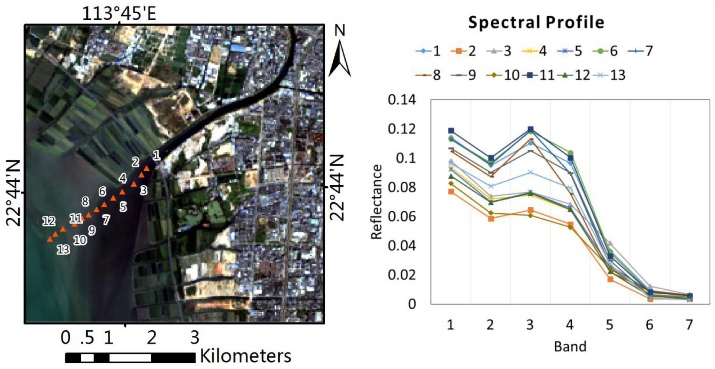
For the surface water, there are more severe spectral variabilities than for other land cover types. This is because the spectral features of surface water are influenced by depth and the aquatic environment. As shown in Figure 3, the spectral features of 13 water pixels varied greatly from pixel to pixel. In order to tackle the high variability of water endmembers, we used a local spatial constraint to dynamically extract the water endmembers. Specifically, the pure water pixels in the nearest spatial neighborhood were considered as the water endmembers for a mixed water–land pixel. Through experimental comparison, the optimal window size was set to 3 × 3. In this work, we used an 8-pixel connected neighborhood system to identify the water endmembers. As shown in Figure 2d, in the 8-pixel neighborhood connected to a water–land mixed pixel located at (k, l), all the pure water pixels were considered to be the water endmembers.
The local MESMA was implemented as follows. Firstly, a spectral endmember library was created by extracting three categories of land endmembers (i.e., vegetation, soil, impervious surfaces), and was derived from Landsat 8 OLI images by using the pixel purity index (PPI) in ENVI v.5.3 [50]. Pixels identified as extreme by the PPI were visually inspected, and the spectra of those which could be classified with confidence as one of the above three land cover components were collected. Count-based endmember selection (CoB), endmember average RMSE (EAR), and minimum average spectral angle (MASA) [45] were used to choose the most suitable endmembers. Secondly, for each mixed water–land pixel, we dynamically selected the water endmembers from Landsat 8 OLI images using a 3 × 3 moving window, where the pure water pixels in the nearest spatial neighborhood were selected as water endmembers for the given mixed pixel. The numbers of land cover endmembers for the three test sites are presented in Table 2. Lastly, we adopted multiple endmember spectral unmixing (based on the linear spectral mixture model) to unmix the mixed water–land pixels. Here, combinations of land and water endmembers were considered, including vegetation–water–shade (V–W–shade), soil–water–shade (S–W–shade), impervious–surfaces–water–shade (I–W–shade), V–S–W–shade, V–I–W–shade, S–I–W–shade, and V–S–I–W–shade. The shade endmember was included in each endmember combination to account for the variation in illumination. Similar to previous studies [47], the following selection criteria were adopted: the fraction values should be between −0.05 and 1.05; the shade fraction value should be below 0.8; and the RMSE should be below 0.025. Among the eligible combinations, the one with the lowest RMSE was considered to be the best endmember combination. If no endmember combination met the RMSE constraint, the pixel was neglected, and the water fraction of the pixel was set to 0.
3.3. Accuracy Assessment
The kappa coefficient (KC) and total error (TE) were calculated to assess the classification accuracy of the developed ABWI. For comparison, the accuracies of NDWI were also obtained. A preliminary test of different water indices, which included the normalized difference water index (NDWI) [23], the modified NDWI (MNDWI) [24], and the automated water extraction index (AWEI) [22], showed that all indices, except the NDWI, had poor performance at our test sites. Therefore, only NDWI was considered for comparison with the ABWI. The ABWI and NDWI were all tested in the optimal threshold.
Root-mean-square error (RMSE) and systematic error (SE) were used to evaluate the accuracy of the water fraction estimated by the proposed SSWE method. The RMSE quantifies the relative error of the estimated land cover fraction, and the SE is used to evaluate the overall trend of the over- or underestimation. For comparison, the accuracy of the automated subpixel water mapping method (ASWM) was also obtained. In order to conduct a comprehensive assessment of the SSWE method, all the pixels, except the 3000 training samples, were used for validation. As the whole sample size was 62,900 in each test site, the validation sample size was 59,900. Here, the water fractions in the pure water pixels and pure land pixels were set to 1 and 0, respectively. The RMSE and SE can be obtained as follows:
where and are the water fraction of the ith pixel of the reference image and estimated image, respectively. N is the number of pixels in the whole image.
4. Results
4.1. Extraction of Pure Water Pixels
Figure 4 shows the pure water pixel extraction results obtained by the proposed ABWI for the three test sites. For comparison, the results obtained by the NDWI are also reported. The visual interpretation indicates that the ABWI shows good performance in extracting pure water pixels. The ABWI is more effective for distinguishing water and mixed water–land pixels than the NDWI (Region 1 and Region 3). Particularly, in the second test set with the Dongbao Estuary, the new index (ABWI) is better at suppressing mud flat and other non-water surface (Region 2).
The accuracies for ABWI and NDWI over the three test sites are shown in Table 3, from which it can be clearly observed that the ABWI achieves better accuracy than the NDWI at all test sites. Overall, the means of the KC and TE achieved by ABWI over the three test sites are 0.957 and 7.56%, respectively, which improves the results provided by NDWI (KC = 0.934, TE = 10.26%). Especially at Dongbao Estuary (with significant presence of mixed water–land pixels and mud flats), the ABWI achieves the largest increments of KC (from 0.912 to 0.945) and the greatest decrements of TE (from 11.67% to 8.16%). Since the NDWI considers only a few bands, the developed all bands water index (ABWI) performs better than the NDWI in the extraction of pure water pixels.
4.2. Subpixel Surface Water Extraction
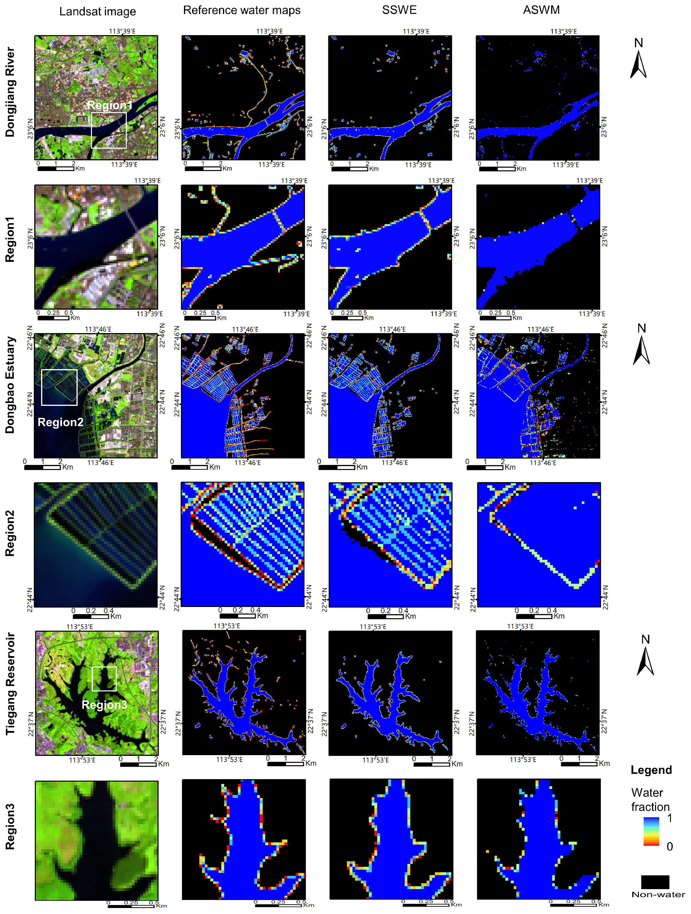
Figure 5 shows the subpixel surface water extraction maps obtained by the proposed SSWE for the three test sites. For comparison, the results obtained by the ASWM method are also reported. Several observations can be obtained according to visual inspection of the obtained results. First of all, it is remarkable that, for the mixed water–land pixels, the SSWE properly extracts the fractions of water in these pixels, which shows clear transitions from water to non-water (Region 1 and Region 3). Furthermore, the SSWE shows very good performance in highly mixed areas, such as the estuary (Region 2). These areas are generally difficult to characterize with the ASWM, mainly due to the complex spectra present in those areas. Finally, it can be observed that both methods fail to identify too narrow rivers and too small waterbodies (width less than 2 pixels). In order to further evaluate the performance of the proposed SSWE, the root-mean-square error (RMSE) and systematic error (SE) were obtained for the three test sites. For comparative purposes, the results obtained from ASWM are also reported. Table 4 indicates that the SSWE reduces RMSE, as compared to the ASWM, for all the three test sites. Especially at Dongbao Estuary (with significant presence of mixed water–land pixels and mud flats), the SSWE achieves the greatest decrements of RMSE (from 0.214 to 0.163). Overall, the mean of the RMSE and SE achieved by SSWE over the three test sites is 0.117 and −0.005, respectively, which improves the results provided by ASWM (RMSE = 0.143, SE = 0.008). Negative SE values are observed for SSWE over all the test sites, indicating that the overall water fraction is underestimated.
5. Discussion
Surface water extraction is a complex problem affected by many factors, especially in estuaries. Since estuaries form a transition zone between river environments and maritime environments, the aquatic environments are complex and highly variable. Mud flats and suspended particulate sediments in estuaries show similar reflectance spectra with their adjacent water pixels, making the water boundaries optical-confused. Meanwhile, there is no distinct rule in the distribution of suspended particulate sediments because of the complicated hydrodynamic conditions in estuaries, which result in high spectral variability of surface water. The results indicate that the SSWE shows better performance than the ASWM in Dongbao Estuary. It can be explained as follows. Firstly, the ABWI using information from all the bands is more effective to distinguish water and non-water pixels than the NDWI, which is used in the ASWM. Secondly, it is difficult for ASWM to extract water–land mixed pixels based on only the spectral information. It seems that SSWE, based on both spectral and spatial information, is a better choice to extract water–land interface mixed pixels. Lastly, the ASWM uses a fixed combination of endmembers and it is limited when mapping land cover with high spectral variability. Thus, the applications of ASWM are limited by high spectral variability of surface water in Dongbao Estuary. As a result, the SSWE integrating the advantages of ABWI and local MESMA appears to be more appropriate in areas that include diverse water types and where the reflectance spectra of surface water are highly variable.
Despite a number of surface water extraction methods reported in the literature, limited research has been undertaken on accuracy assessment using high spatial resolution reference images acquired on the same day with Landsat 8 OLI data. This is particularly important when a subpixel water extraction method is developed. Given that water conditions are sometimes changing rapidly, short or no time span between reference data and Landsat 8 OLI data is essential for producing the “true” water map, especially when the bank is not artificial. For instance, in coastal areas, the surface water changes with the tide. If the reference image is not acquired at the same time as Landsat 8 OLI data, a bias in the surface water boundaries could arise, since tides influence the water level. However, the short time span between reference data and Landsat 8 OLI data is inevitable. In order to minimize the bias in the surface water boundaries and guarantee a convincing validation, the SSWE is evaluated using reference data acquired on the same day with Landsat 8 OLI data.
In the task of surface water extraction from a large data set of images, an automated process is preferred. Though only the second step of SSWE is automatically implemented in this work, the three-step strategy in SSWE has the potential to perform automated water extraction. First of all, the pure water pixels can be extracted automatically based on the histogram of ABWI using the method of Xie et al. [42]. This method was tested in the ABWI image histogram of our three test sites to extract pure water pixels, and the corresponding kappa coefficients were a little less than that of the optimal threshold. Furthermore, in the third step of SSWE, the land endmembers are able to be extracted automatically from the image with the land mask produced from the first two steps by using the methods proposed by Somers et al. [55]. Besides, in situ data is not required in the SSWE method. Thus, the whole procedure of SSWE can be automated. Nevertheless, the performance of the automated process needs to be evaluated.
Although our new water extraction method has been tested in three test sites with different surface water types and achieves promising performance, further studies should be conducted in order to improve the robustness of the proposed method. At this stage, the problem of too narrow rivers and too small waterbodies (width less than 2 pixels) has not yet been taken into account. Despite that methods reported in the literature [28,36] can partially detect these pixels, extraction of these pixels is still a challenge. To accurately identify water fraction in these pixels, it is crucial to collect the most representative water endmember. However, because of little or no pure water pixels adjacent to these pixels, the selection of the most representative water endmember remains a difficulty. In the future, we will extend the capacity of the SSWE to extract these waterbodies. The ABWI will be also tested in other water types for water extraction purpose. Furthermore, since the SSWE was designed on the basis of the land cover reflectance and local spatial constraints, its application can be extended to satellite image types with similar spectral bands. The SSWE will be tested in additional sites and other satellite image types with similar spectral bands, such as Sentinel-2 MSI images, to validate its performance and robustness.
6. Conclusions
In this study, we developed a new subpixel surface water extraction (SSWE) method for Landsat 8 OLI data that is able to improve the extraction of surface water in mixed water–land pixels by means of subpixel analysis. Specifically, we first developed an all bands water index (ABWI) to extract the pure water pixels. The ABWI takes full advantage of the multispectral bands and mines more information than the previous water indices. Results indicated that the ABWI performed reasonably well in pure water pixel extraction. Then, we developed a local multiple endmember spectral mixture analysis (MESMA) to identify water fractions at mixed water–land pixels. By incorporating a local MESMA, the proposed SSWE dynamically characterizes the high spectral variability of the water endmembers and complex land classes. The proposed method considered the nearest pure water pixels as water endmembers, and further allowed the number and type of endmembers to vary on a per-pixel basis. Our experimental results with three different test sites in China indicated that the newly developed SSWE exhibited very good performance, with an average root-mean-square error of 0.117. A thorough comparison with the automated subpixel water mapping method (ASWM) indicated that our SSWE outperformed the method in most cases. Especially at Dongbao Estuary (with significant presence of mixed water–land pixels and mud flats), the SSWE achieved the greatest decrements of RMSE. Therefore, the SSWE can be used to extract surface water with high accuracy, especially in areas with optically complex aquatic environments.
Author Contributions
L.X. designed and conducted the overall research, experiment and analysis, and prepared the manuscript. R.D. and J.L. led this research and reviewed the manuscript. X.L. supported the reference data collection. Y.Q. helped perform the analysis with constructive discussions. Y.L. supported the Landsat data collection. Y.L. joined the experiment. All authors wrote the paper.
Acknowledgments
The research was supported by the Science and Technology Planning Project of Guangdong Province (grant Nos. 2017B020216001 and 2016A020222006), the Young teacher development program of Sun Yat-sen University (grant No. 17lgpy41), the Irrigation works science and technology innovation project of Guangdong Province (No. 2014-13) and the China Postdoctoral Science Foundation (grant No. 2017M612792). We gratefully thank the editors and the anonymous reviewers for their helpful comments.
Conflicts of Interest
The authors declare no conflict of interest.
References
- Postel, S.L. Entering an era of water scarcity: The challenges ahead. Ecol. Appl. 2000, 10, 941–948. [Google Scholar] [CrossRef]
- Duker, L.; Borre, L. Biodiversity Conservation of the World’s Lakes: A Preliminary Framework for Identifying Priorities; LakeNet Report Series, Number 2; Monitor International: Annapolis, MD, USA, 2001. [Google Scholar]
- McGwire, K.; Minor, T.; Fenstermaker, L. Hyperspectral mixture modeling for quantifying sparse vegetation cover in arid environments. Remote Sens. Environ. 2000, 72, 360–374. [Google Scholar] [CrossRef]
- Huang, Y.; Chen, X.; Li, Y.; Willems, P.; Liu, T. Integrated modeling system for water resources management of Tarim River basin. Environ. Eng. Sci. 2010, 27, 255–269. [Google Scholar] [CrossRef]
- Lacava, T.; Filizzola, C.; Pergola, N.; Sannazzaro, F.; Tramutoli, V. Improving flood monitoring by the Robust AVHRR Technique (RAT) approach: The case of the April 2000 Hungary flood. Int. J. Remote Sens. 2010, 31, 2043–2062. [Google Scholar] [CrossRef]
- Richter, B.D.; Mathews, R.; Wigington, R. Ecologically sustainable water management: Managing river flows for ecological integrity. Ecol. Appl. 2003, 13, 206–224. [Google Scholar] [CrossRef]
- Viala, E. Water for food, water for life a comprehensive assessment of water management in agriculture. Irrig. Drain. Syst. 2008, 22, 127–129. [Google Scholar] [CrossRef]
- Palmer, S.C.J.; Kutser, T.; Hunter, P.D. Remote sensing of inland waters: Challenges, progress and future directions. Remote Sens. Environ. 2015, 157, 1–8. [Google Scholar] [CrossRef]
- Pekel, J.F.; Vancutsem, C.; Bastin, L.; Clerici, M.; Vanbogaert, E.; Bartholomé, E.; Defourny, P. A near real-time water surface detection method based on HSV transformation of MODIS multi-spectral time series data. Remote Sens. Environ. 2014, 140, 704–716. [Google Scholar] [CrossRef]
- Sharma, R.; Tateishi, R.; Hara, K.; Nguyen, L. Developing superfine water index (SWI) for global water cover mapping using MODIS data. Remote Sens. 2015, 7, 13807–13841. [Google Scholar] [CrossRef]
- Jawak, S.D.; Luis, A.J. A semiautomatic extraction of Antarctic lake features using Worldview-2 imagery. Photogramm. Eng. Remote Sens. 2014, 80, 939–952. [Google Scholar] [CrossRef]
- Fisher, A.; Danaher, T. A water index for SPOT5 HRG satellite imagery, New South Wales, Australia, determined by linear discriminant analysis. Remote Sens. 2013, 5, 5907–5925. [Google Scholar] [CrossRef]
- Chen, W.; Doko, T.; Fukui, H.; Yan, W. Changes in Imja Lake and Karda Lake in the Everest Region of Himalaya. Nat. Resour. 2013, 4, 449–455. [Google Scholar] [CrossRef]
- Bryant, R.G.; Rainey, M.P. Investigation of flood inundation on playas within the Zone of Chotts, using a time-series of AVHRR. Remote Sens. Environ. 2002, 82, 360–375. [Google Scholar] [CrossRef]
- Frazier, P.S.; Page, K.J. Water body detection and delineation with Landsat TM data. Photogramm. Eng. Remote Sens. 2000, 66, 1461–1467. [Google Scholar]
- Yang, Y.; Liu, Y.; Zhou, M.; Zhang, S.; Zhan, W.; Sun, C.; Duan, Y. Landsat 8 OLI image based terrestrial water extraction from heterogeneous backgrounds using a reflectance homogenization approach. Remote Sens. Environ. 2015, 171, 14–32. [Google Scholar] [CrossRef]
- Lu, S.; Wu, B.; Yan, N.; Wang, H. Water body mapping method with HJ-1A/B satellite imagery. Int. J. Appl. Earth Obs. 2011, 13, 428–434. [Google Scholar] [CrossRef]
- Yao, F.; Wang, C.; Dong, D.; Luo, J.; Shen, Z.; Yang, K. High-resolution mapping of urban surface water using ZY-3 multi-spectral imagery. Remote Sens. 2015, 7, 12336–12355. [Google Scholar] [CrossRef]
- Pahlevan, N.; Lee, Z.; Wei, J.; Schaaf, C.B.; Schott, J.R.; Berk, A. On-orbit radiometric characterization of OLI (Landsat-8) for applications in aquatic remote sensing. Remote Sens. Environ. 2014, 154, 272–284. [Google Scholar] [CrossRef]
- Jain, S.K.; Singh, R.D.; Jain, M.K.; Lohani, A.K. Delineation of flood-prone areas using remote sensing techniques. Water Resour. Manag. 2005, 19, 333–347. [Google Scholar] [CrossRef]
- Ryu, J.; Won, J.; Min, K.D. Waterline extraction from Landsat TM data in a tidal flat: A case study in Gomso Bay, Korea. Remote Sens. Environ. 2002, 83, 442–456. [Google Scholar] [CrossRef]
- Feyisa, G.L.; Meilby, H.; Fensholt, R.; Proud, S.R. Automated Water Extraction Index: A new technique for surface water mapping using Landsat imagery. Remote Sens. Environ. 2014, 140, 23–35. [Google Scholar] [CrossRef]
- McFeeters, S.K. The use of the Normalized Difference Water Index (NDWI) in the delineation of open water features. Int. J. Remote Sens. 1996, 17, 1425–1432. [Google Scholar] [CrossRef]
- Xu, H. Modification of normalised difference water index (NDWI) to enhance open water features in remotely sensed imagery. Int. J. Remote Sens. 2006, 27, 3025–3033. [Google Scholar] [CrossRef]
- Daya Sagar, B.S.; Gandhi, G.; Prakasa Rao, B.S. Applications of mathematical morphology in surface water body studies. Int. J. Remote Sens. 1995, 16, 1495–1502. [Google Scholar] [CrossRef]
- Blaschke, T. Object based image analysis for remote sensing. ISPRS J. Photogramm. Remote Sens. 2010, 65, 2–16. [Google Scholar] [CrossRef]
- Cai, Y.; Sun, G.; Liu, B. Mapping of water body in Poyang Lake from partial spectral unmixing of MODIS data. In Proceedings of the 2005 IEEE International Geoscience and Remote Sensing Symposium (IGARSS’05), Seoul, Korea, 25–29 July 2005; pp. 4539–4540. [Google Scholar]
- Ji, L.; Gong, P.; Geng, X.; Zhao, Y. Improving the accuracy of the water surface cover type in the 30 m FROM-GLC product. Remote Sens. 2015, 7, 13507–13527. [Google Scholar] [CrossRef]
- Liu, Y.; Chen, X.; Yang, Y.; Sun, C.; Zhang, S. Automated extraction and mapping for desert wadis from Landsat imagery in arid West Asia. Remote Sens. 2016, 8, 246:1–246:23. [Google Scholar] [CrossRef]
- Jiang, H.; Feng, M.; Zhu, Y.; Lu, N.; Huang, J.; Xiao, T. An automated method for extracting rivers and lakes from Landsat imagery. Remote Sens. 2014, 6, 5067–5089. [Google Scholar] [CrossRef]
- Sethre, P.R.; Rundquist, B.C.; Todhunter, P.E. Remote detection of prairie pothole ponds in the Devils Lake Basin, North Dakota. Gisci. Remote Sens. 2005, 42, 277–296. [Google Scholar] [CrossRef]
- Verpoorter, C.; Kutser, T.; Tranvik, L. Automated mapping of water bodies using Landsat multispectral data. Limnol. Oceanogr. Methods 2012, 10, 1037–1050. [Google Scholar] [CrossRef]
- Yang, K.; Li, M.; Liu, Y.; Cheng, L.; Duan, Y.; Zhou, M. River Delineation from Remotely Sensed Imagery Using a Multi-Scale Classification Approach. IEEE J. Sel. Top. Appl. Earth Obs. Remote Sens. 2014, 7, 4726–4737. [Google Scholar] [CrossRef]
- Ji, L.; Zhang, L.; Wylie, B. Analysis of dynamic thresholds for the normalized difference water index. Photogramm. Eng. Remote Sens. 2009, 75, 1307–1317. [Google Scholar] [CrossRef]
- Jia, K.; Jiang, W.; Li, J.; Tang, Z. Spectral matching based on discrete particle swarm optimization: A new method for terrestrial water body extraction using multi-temporal Landsat 8 images. Remote Sens. Environ. 2018, 209, 1–18. [Google Scholar] [CrossRef]
- Huang, C.; Peng, Y.; Lang, M.; Yeo, I.; McCarty, G. Wetland inundation mapping and change monitoring using Landsat and airborne LiDAR data. Remote Sens. Environ. 2014, 141, 231–242. [Google Scholar] [CrossRef]
- Jin, H.; Huang, C.; Lang, M.W.; Yeo, I.; Stehman, S.V. Monitoring of wetland inundation dynamics in the Delmarva Peninsula using Landsat time-series imagery from 1985 to 2011. Remote Sens. Environ. 2017, 190, 26–41. [Google Scholar] [CrossRef]
- Reschke, J.; Hüttich, C. Continuous field mapping of Mediterranean wetlands using sub-pixel spectral signatures and multi-temporal Landsat data. Int. J. Appl. Earth Obs. 2014, 28, 220–229. [Google Scholar] [CrossRef]
- Halabisky, M.; Moskal, L.M.; Gillespie, A.; Hannam, M. Reconstructing semi-arid wetland surface water dynamics through spectral mixture analysis of a time series of Landsat satellite images (1984–2011). Remote Sens. Environ. 2016, 177, 171–183. [Google Scholar] [CrossRef]
- Sun, W.; Du, B.; Xiong, S. Quantifying sub-pixel surface water coverage in urban environments using low-albedo fraction from Landsat imagery. Remote Sens. 2017, 9, 428:1–428:15. [Google Scholar] [CrossRef]
- Verhoeye, J.; Wulf, R.D. Land cover mapping at sub-pixel scales using linear optimization techniques. Remote Sens. Environ. 2002, 79, 96–104. [Google Scholar] [CrossRef]
- Xie, H.; Luo, X.; Xu, X.; Pan, H.; Tong, X. Automated subpixel surface water mapping from heterogeneous urban environments using Landsat 8 OLI imagery. Remote Sens. 2016, 8, 584:1–584:16. [Google Scholar] [CrossRef]
- Roberts, D.A.; Gardner, M.; Church, R.; Ustin, S.; Scheer, G.; Green, R.O. Mapping chaparral in the Santa Monica Mountains using multiple endmember spectral mixture models. Remote Sens. Environ. 1998, 65, 267–279. [Google Scholar] [CrossRef]
- Dudley, K.L.; Dennison, P.E.; Roth, K.L.; Roberts, D.A.; Coates, A.R. A multi-temporal spectral library approach for mapping vegetation species across spatial and temporal phenological gradients. Remote Sens. Environ. 2015, 167, 121–134. [Google Scholar] [CrossRef]
- Fernandez-Manso, A.; Quintano, C.; Roberts, D.A. Burn severity influence on post-fire vegetation cover resilience from Landsat MESMA fraction images time series in Mediterranean forest ecosystems. Remote Sens. Environ. 2016, 184, 112–123. [Google Scholar] [CrossRef]
- Painter, T.H.; Rittger, K.; McKenzie, C.; Slaughter, P.; Davis, R.E.; Dozier, J. Retrieval of subpixel snow covered area, grain size, and albedo from MODIS. Remote Sens. Environ. 2009, 113, 868–879. [Google Scholar] [CrossRef]
- Powell, R.; Roberts, D.; Dennison, P.; Hess, L. Sub-pixel mapping of urban land cover using multiple endmember spectral mixture analysis: Manaus, Brazil. Remote Sens. Environ. 2007, 106, 253–267. [Google Scholar] [CrossRef]
- EarthExplorer. Available online: http://earthexplorer.usgs.gov (accessed on 5 May 2016).
- Roy, D.P.; Wulder, M.A.; Loveland, T.R.; Woodcock, C.E.; Allen, R.G.; Anderson, M.C.; Helder, D.; Irons, J.R.; Johnson, D.M.; Kennedy, R.; et al. Landsat-8: Science and product vision for terrestrial global change research. Remote Sens. Environ. 2014, 145, 154–172. [Google Scholar] [CrossRef]
- Harris Geospatial Solutions. Available online: http://www.harrisgeospatial.com (accessed on 11 May 2017).
- Help Articles. Available online: http://www.harrisgeospatial.com/Support/SelfHelpTools/HelpArticles.aspx (accessed on 19 May 2017).
- NASA Goddard Space Flight Center for Aerosol Optical Depth. Available online: http://aeronet.gsfc.nasa.gov/new_web/aerosols.html (accessed on 16 May 2016).
- Fisher, A.; Flood, N.; Danaher, T. Comparing Landsat water index methods for automated water classification in eastern Australia. Remote Sens. Environ. 2016, 175, 167–182. [Google Scholar] [CrossRef]
- Adams, J.B.; Smith, M.O.; Gillespie, A.R.; Adams, J.B.; Smith, M.O. Imaging spectroscopy: Interpretation based on spectral mixture analysis. In Remote Geochemical Analysis: Elemental and Mineralogical Composition. Topics in Remote Sensing 4; Pieters, C.M., Englert, P., Eds.; Cambridge University Press: New York, NY, USA, 1993; pp. 145–166. [Google Scholar]
- Somers, B.; Zortea, M.; Plaza, A.; Asner, G.P. Automated extraction of image-based endmember bundles for improved spectral unmixing. IEEE J. Sel. Top. Appl. Earth Obs. Remote Sens. 2012, 5, 396–408. [Google Scholar] [CrossRef]
Figure 1.
Three considered test sites in Guangdong, China. (a) Location of the test sites; (b) false color image (formed using bands 6, 5, and 4 as red, green, and blue) of Test Site 1; (c) false color image of Test Site 2; (d) false color image of Test Site 3.
Figure 1.
Three considered test sites in Guangdong, China. (a) Location of the test sites; (b) false color image (formed using bands 6, 5, and 4 as red, green, and blue) of Test Site 1; (c) false color image of Test Site 2; (d) false color image of Test Site 3.
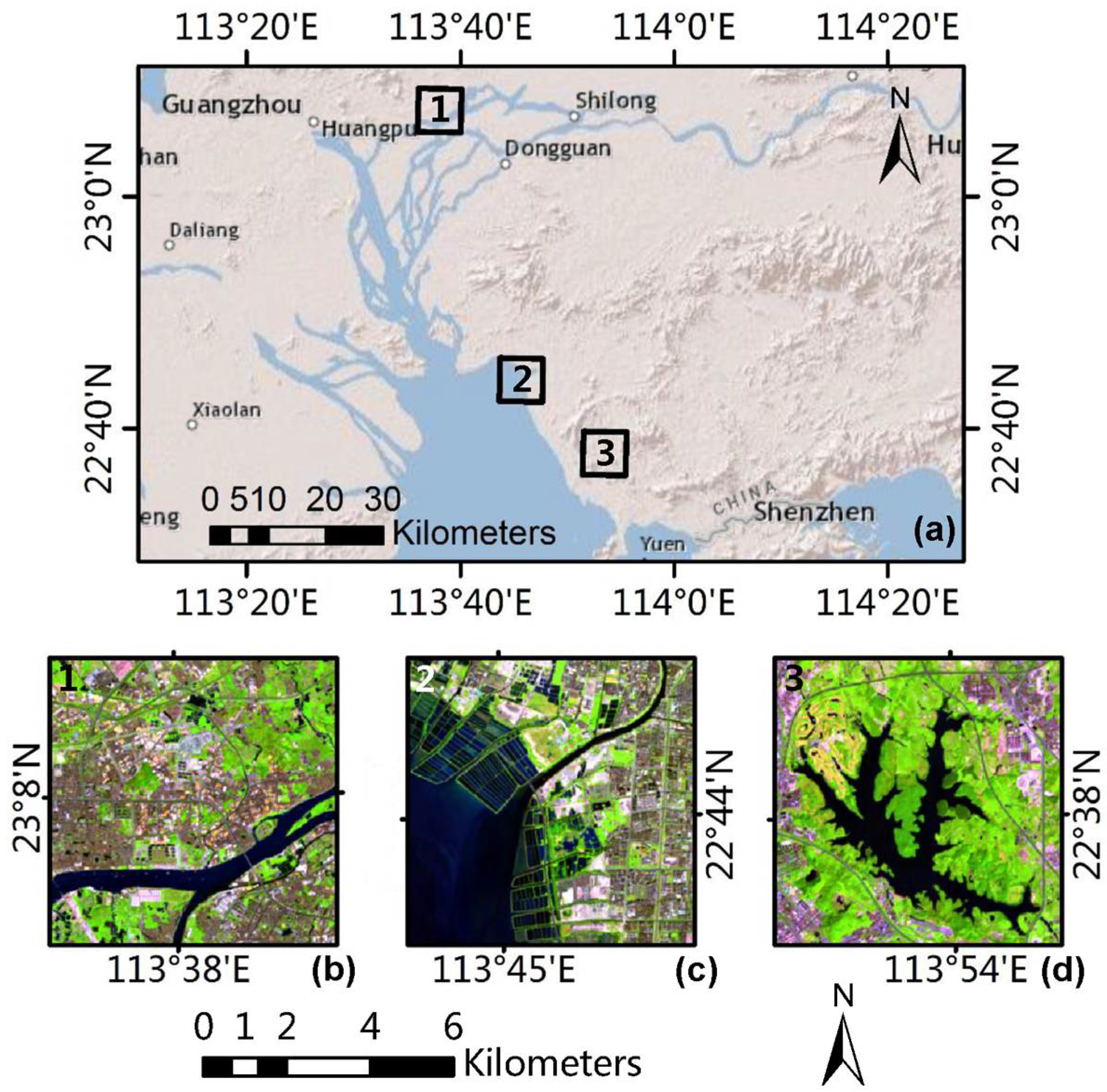
Figure 2.
Conceptual graph of extraction of pure water pixels and mixed water–land pixels and selection of water endmembers. (a) Grid superimposed on a high spatial resolution image obtained through Google Earth™; (b) water and land classification result; (c) mixed water–land pixels extraction; (d) water endmember selection by a 3 × 3 moving window.
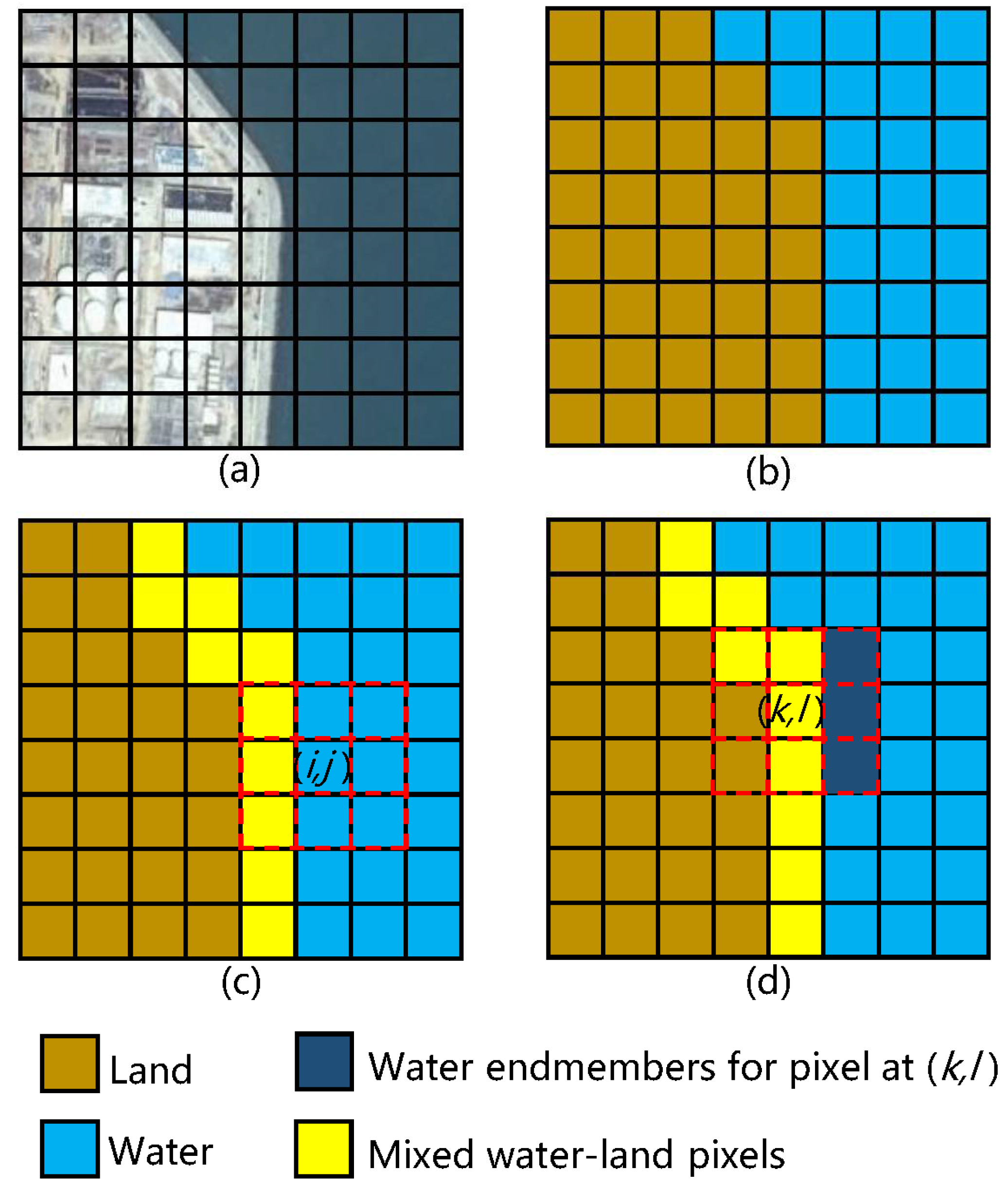
Figure 3.
Illustration of the spectral variability in surface water. A true color image (using bands 4, 3, and 2 as red, green, and blue) for Test Site 2 is provided in the leftmost part of the figure, where spatially remarkable color changes can be appreciated for the surface water. The spectral profile of 13 water pixels located at the leftmost image is presented in the plot at the rightmost part of the figure.

Figure 4.
Pure water pixels extraction maps of the all bands water index (ABWI) and normalized difference water index (NDWI) for the three test sites.
Figure 4.
Pure water pixels extraction maps of the all bands water index (ABWI) and normalized difference water index (NDWI) for the three test sites.
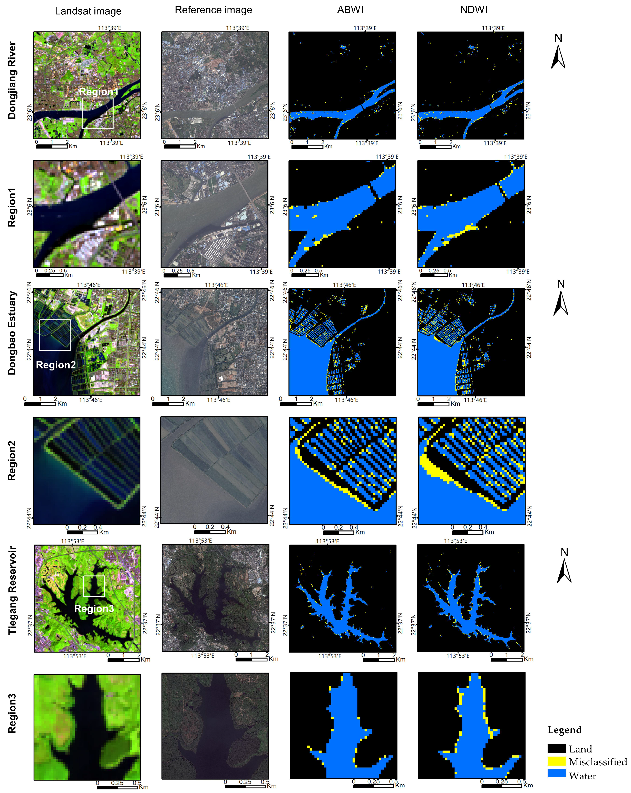
Figure 5.
Comparison of surface water extraction results of the subpixel surface water extraction (SSWE) and the automated subpixel water mapping method (ASWM) for the three test sites. The color range indicates the range of water fractions (i.e., blue indicates pure water pixels and red indicates pixels with low water fractions). Dark indicates non-water pixels.


Table 1.
Summary of the Landsat 8 Operational Land Imager (OLI) images used in the present study.
| Test Sites | Path/Row | Acquisition Date | Landsat Scene ID | Cloud Cover |
|---|---|---|---|---|
| East River | 122/44 | 2 October 2015 | LC81220442015275 | 19.61% |
| Dongbao Estuary | 122/44 | 16 November 2014 | LC81220442014320 | 8.90% |
| Tiegang Reservoir | 122/44 | 18 October 2015 | LC81220442015291 | 1.15% |
Table 2.
Number of land cover endmembers for the three test sites.
| Test Sites | Water | Vegetation | Impervious Surface | Soil |
|---|---|---|---|---|
| Dongjiang River | 1533 | 6 | 8 | 5 |
| Dongbao Estuary | 4568 | 5 | 7 | 7 |
| Tiegang Reservoir | 2097 | 8 | 5 | 4 |
Table 3.
The kappa coefficient (KC) and total error (TE) obtained by the two water indices for the three considered test sites. ABWI: all bands water index; NDWI: normalized difference water index.
Table 3.
The kappa coefficient (KC) and total error (TE) obtained by the two water indices for the three considered test sites. ABWI: all bands water index; NDWI: normalized difference water index.
| Test Sites | KC | TE (%) | ||
|---|---|---|---|---|
| ABWI | NDWI | ABWI | NDWI | |
| Dongjiang River | 0.952 | 0.931 | 9.83 | 12.41 |
| Dongbao Estuary | 0.945 | 0.912 | 8.16 | 11.67 |
| Tiegang Reservoir | 0.973 | 0.960 | 4.68 | 6.72 |
| Average | 0.957 | 0.934 | 7.56 | 10.26 |
Table 4.
Root-mean-square error (RMSE) and systematic error (SE) obtained by the two surface water extraction methods for the three considered test sites. ASWM: automated subpixel water mapping method; SSWE: subpixel surface water extraction.
Table 4.
Root-mean-square error (RMSE) and systematic error (SE) obtained by the two surface water extraction methods for the three considered test sites. ASWM: automated subpixel water mapping method; SSWE: subpixel surface water extraction.
| Test Sites | SE | RMSE | ||
|---|---|---|---|---|
| SSWE | ASWM | SSWE | ASWM | |
| Dongjiang River | −0.005 | −0.013 | 0.110 | 0.129 |
| Dongbao Estuary | −0.007 | 0.047 | 0.163 | 0.214 |
| Tiegang Reservoir | −0.005 | −0.010 | 0.085 | 0.087 |
| Average | −0.005 | 0.008 | 0.117 | 0.143 |
© 2018 by the authors. Licensee MDPI, Basel, Switzerland. This article is an open access article distributed under the terms and conditions of the Creative Commons Attribution (CC BY) license (http://creativecommons.org/licenses/by/4.0/).
Share and Cite
MDPI and ACS Style
Xiong, L.; Deng, R.; Li, J.; Liu, X.; Qin, Y.; Liang, Y.; Liu, Y. Subpixel Surface Water Extraction (SSWE) Using Landsat 8 OLI Data. Water 2018, 10, 653. https://doi.org/10.3390/w10050653
AMA Style
Xiong L, Deng R, Li J, Liu X, Qin Y, Liang Y, Liu Y. Subpixel Surface Water Extraction (SSWE) Using Landsat 8 OLI Data. Water. 2018; 10(5):653. https://doi.org/10.3390/w10050653
Chicago/Turabian StyleXiong, Longhai, Ruru Deng, Jun Li, Xulong Liu, Yan Qin, Yeheng Liang, and Yingfei Liu. 2018. "Subpixel Surface Water Extraction (SSWE) Using Landsat 8 OLI Data" Water 10, no. 5: 653. https://doi.org/10.3390/w10050653
Note that from the first issue of 2016, this journal uses article numbers instead of page numbers. See further details here.