Experimental and Numerical Study of Free-Surface Flows in a Corrugated Pipe
by
 , ,
, ,
Francesco Calomino
*, 
Giancarlo Alfonsi
,
Roberto Gaudio
 ,
,
Antonino D’Ippolito
,
Agostino Lauria
, 
Ali Tafarojnoruz
and
Serena Artese
Dipartimento di Ingegneria Civile, Università della Calabria, Via P. Bucci, Cubo 42b, 87036 Rende, Italy
*
Author to whom correspondence should be addressed.
Water 2018, 10(5), 638; https://doi.org/10.3390/w10050638
Submission received: 4 April 2018
/
Revised: 7 May 2018
/
Accepted: 8 May 2018
/
Published: 15 May 2018
(This article belongs to the Section Hydraulics and Hydrodynamics)
Abstract
:A new discharge computational model is proposed on the basis of the integration of the velocity profile across the flow cross-section in an internally corrugated pipe flowing partially full. The model takes into account the velocity profiles in the pressurised pipe to predict the flow rate under free-surface flow conditions. The model was evaluated through new laboratory experiments as well as a literature datasets. The results show that flow depth and pipe slope may affect the model accuracy; nevertheless, a prediction error smaller than 20% is expected from the model. Experimental results reveal the influence of the pipe slope and flow depth on the friction factor and the stage-discharge curves: the friction factor may increase with pipe slope, while it reduces as flow depth increases. Hence, a notable change of pipe slope may lead to the variation of the stage-discharge curve. A part of this study deals with numerical simulation of the velocity profiles and the stage-discharge curves. Using the Reynolds-Averaged Navier-Stokes (RANS) equations, numerical solutions were obtained to simulate four experimental tests, obtaining enough accurate results as to velocity profiles and water depths. The results of the simulated flow velocity were used to estimate the flow discharge, confirming the potential of numerical techniques for the prediction of stage-discharge curves.
1. Introduction
Free-surface flow in corrugated pipes is a topic of interest for culvert and drain design. Culverts traditionally are made of large corrugated steel pipes, whose surface is corrugated because of static reasons. In high-slope drains, internally corrugated plastic pipes are commonly implemented: the internal corrugation reduces the flow velocities so that drop manholes are unnecessary.
A correct estimation of a head loss parameter in the form of Darcy’s friction factor or Manning’s roughness coefficient is crucial for the practical design of corrugated pipes. In this context, Morris [1,2] was among the pioneers who made an effort to extract equations and diagrams to estimate the flow friction factor in corrugated pipes. Nevertheless, in the past decades when his method was evaluated it could not demonstrate satisfactory predictions of friction factors, in particular for small discharges [3,4]. Furthermore, the proposed method by Morris [1] was originally derived for axial or two-dimensional flow conditions. These conditions should still be checked since it is possible that the velocity pattern in a free-surface pipe flow is not essentially 2D.
Previous studies on the friction factor and flow velocity profiles of corrugated pipes were mainly conducted under pressurised pipe flow conditions: a comprehensive literature review is available in Reference [4]. On the other hand, there are few studies on the friction factor and velocity profiles of corrugated pipes under free-surface flow conditions. The following paragraphs point to the previous studies on the hydraulics of corrugated pipes under free-surface flow conditions.
An earlier study on flow resistance of three relatively large corrugated pipes under both full-pipe and free-surface flow conditions was performed by Webster and Metcalf [5]. The employed pipes were 3, 5, and 7 ft in diameter. That study mainly focused on the velocity profile and friction factor of the selected pipes under full-pipe flow conditions with less attention to the flow resistance of the pipes under free-surface flow. Nevertheless, the finding of Webster and Metcalf [5] about the value of Manning’s n when the pipes convey the flow under free-surface conditions is quite interesting: they concluded that Manning’s n for free-surface flow is almost independent of the flow depth and is around the value of 0.024 s/m1/3 obtained for full-pipe flow conditions.
Ead et al. [6] derived empirical equations to predict the flow velocity pattern within a steel corrugated pipe. The measurement of the velocity profiles was conducted at the pipe centreline axis as well as at the different lateral distances from the central vertical plane. Ead et al. [6] reported that the well-known Prandtl equation for the rough wall is valid to predict the velocity profile at a region near the corrugations, whereas, after a certain distance from the corrugations, there would be a deviation from the logarithmic line. The proposed equations by Ead et al. [6] may be used to predict the location where the velocity data points initiate to deviate from the Prandtl equation, the magnitude of the deviation from the logarithmic line at each distance from the corrugation elements and the maximum deviation of the velocity profile from the logarithmic line. Those authors also reported that their findings agree with the dataset of a much larger pipe. Nevertheless, further study is needed to ensure if the proposed equations are universally valid for all the corrugated pipes.
Giustolisi et al. [7] presented the results of a series of tests on three corrugated plastic pipes. Water depths h and discharges Q were recorded for several slopes i ranging from 3.5% to 17.5%. Their results show that the Manning roughness coefficient varies with flow depth and pipe slope. They also introduced empirical equations for the friction factor of each pipe as well as one equation for all the three tested pipes.
Analysis of 3D velocity data of a corrugated pipe under the free-surface flow condition by Clark and Kehler [8] clarifies the existence of secondary currents, which contribute to the strong velocity dip at the flow surface. The experiments by Clark and Kehler [8], conducted at relatively small slopes (ranging from 0.028% to 0.27%), show similar shapes of the shear stress distributions for all the designed slopes. The maximum shear stress for all tests was observed at the pipe centreline, being around 10% larger than the mean shear stress. Moreover, Clark and Kehler [8] pointed out a notable portion of the cross-sectional flow area with streamwise velocity smaller than the mean bulk flow velocity. This area was observed within the 20% of the flow depth in the vicinity of the corrugated culvert wall: identifying this low-velocity area is useful for fish passage regulations.
This study focuses on the hydraulic characteristics of a corrugated pipe under free-surface flow conditions. In this case, a general law involves three flow variables (that is, the flow velocity, flow depth, and energy grade line) as well as the pipe wall nature and geometry. Unfortunately, the wall geometry cannot be easily expressed, since it involves at least the corrugation depth, the spacing between corrugation crests, and the corrugation curvature. In addition, the pipe used for the laboratory tests is smaller than those used for practical purposes, which of course makes it impossible to get the complete similarity between the model and prototype and also makes it difficult to find the limit between the hyper-turbulent flow and other flow regimes that may occur in the corrugated pipes.
The hydraulics of the selected pipe in the present study were previously investigated under pressure by Calomino et al. [4]. The main objectives of performing new tests in the present study are (1) to compare the friction factor of a corrugated pipe under the free-surface flow condition with that of the pressurised pipe flow; (2) to consider the influence of the pipe slope on the stage-discharge curves; (3) to develop a simple analytical model to predict the flow rate on the basis of the pressurised flow velocity profiles, that can be easily provided by the pipe producers; and (4) to predict flow velocity profiles by means of numerical simulation and evaluate the accuracy of two turbulence closure models.
2. Materials and Methods
This section describes the details of the experimental facilities and procedure, the formulation of a new analytical model to calculate pipe flow discharge, and the identification of the selected numerical model.
2.1. Experimental Set-Up and Tests
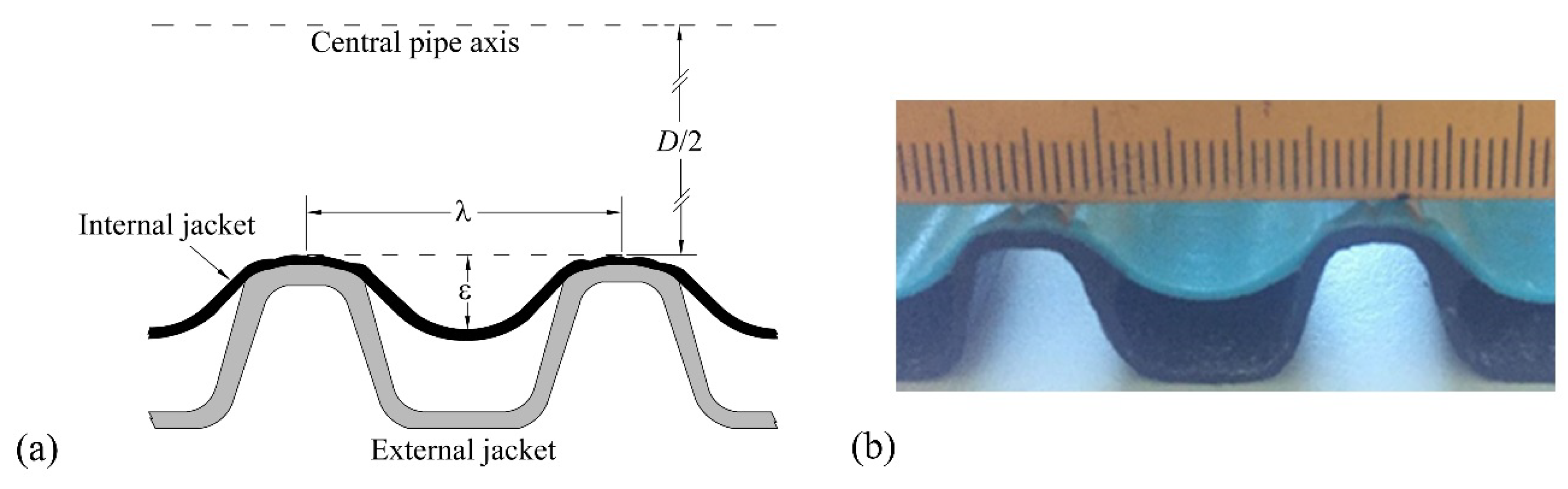
A series of hydraulic tests were performed in the Laboratorio “Grandi Modelli Idraulici”, University of Calabria, Italy, using an internally corrugated plastic pipe with a minimum internal diameter D = 17.1 cm. The main geometric parameters of the pipe were the roughness height ε = 0.6 cm and the longitudinal spacing of the roughness elements λ = 2.54 cm (Figure 1). The pipe was 15.85 m long and placed on a steel truss, whose slope can be set to the required value. All the tests of this study were conducted under free-surface flow conditions.
The pipe was fed by means of the laboratory circuit. A 1–2% accurate V-notch Thomson were mounted in a metallic caisson or a 1–2% accurate Bazin weir, that is, a sharp-crested rectangular weir, installed in a restitution channel allowed the discharge measurement. Small discharges (Q < 4 L/s) were accurately estimated through a relationship previously obtained from the water levels upstream to the Thomson weir and a calibrated volumetric tank. To measure the water levels along the pipe, 10 observation ports, around 120 cm distant from each other, were cut on the upper part of the pipe (Figure 2).
At the pipe bottom, in the middle of each window, a pressure tap was installed at the trough of a corrugation element and connected to a 1 cm diameter flexible pipe. Each flexible pipe was linked to a manifold through a separate valve. The instantaneous water pressure at each pressure tap was captured by means of a Druck pressure transducer at the manifold extremity and recorded with a data acquisition system set to a frequency of 50 Hz. Preliminary tests clarified that a sampling duration of 30 s is adequate to obtain a stable time-averaged pressure head at the pressure taps. Before running the experiments, the pressure transducer signal was accurately calibrated with water levels at a vertically placed cylinder. The water level within the cylinder was measured using a point gauge with the accuracy of 0.1 mm. The experimental campaign can be divided into two parts:
For the first part of the experiments, a total number of 34 tests was performed by changing the pipe slope (i = 1.5%, 3.5% and 7.0%) and flow depth. During each test, the water surface level was estimated by means of the measured pressure values. The water surface slope was also checked to be the same as the bottom slope, ensuring the uniformity of the flow depth. For each test, after setting the pipe slope, the flow discharge Q and the flow depth h were measured to calculate the bulk mean flow velocity U = Q/A, where A is the cross-sectional flow area, the hydraulic radius Rh, and the Darcy-Weisbach friction factor f.
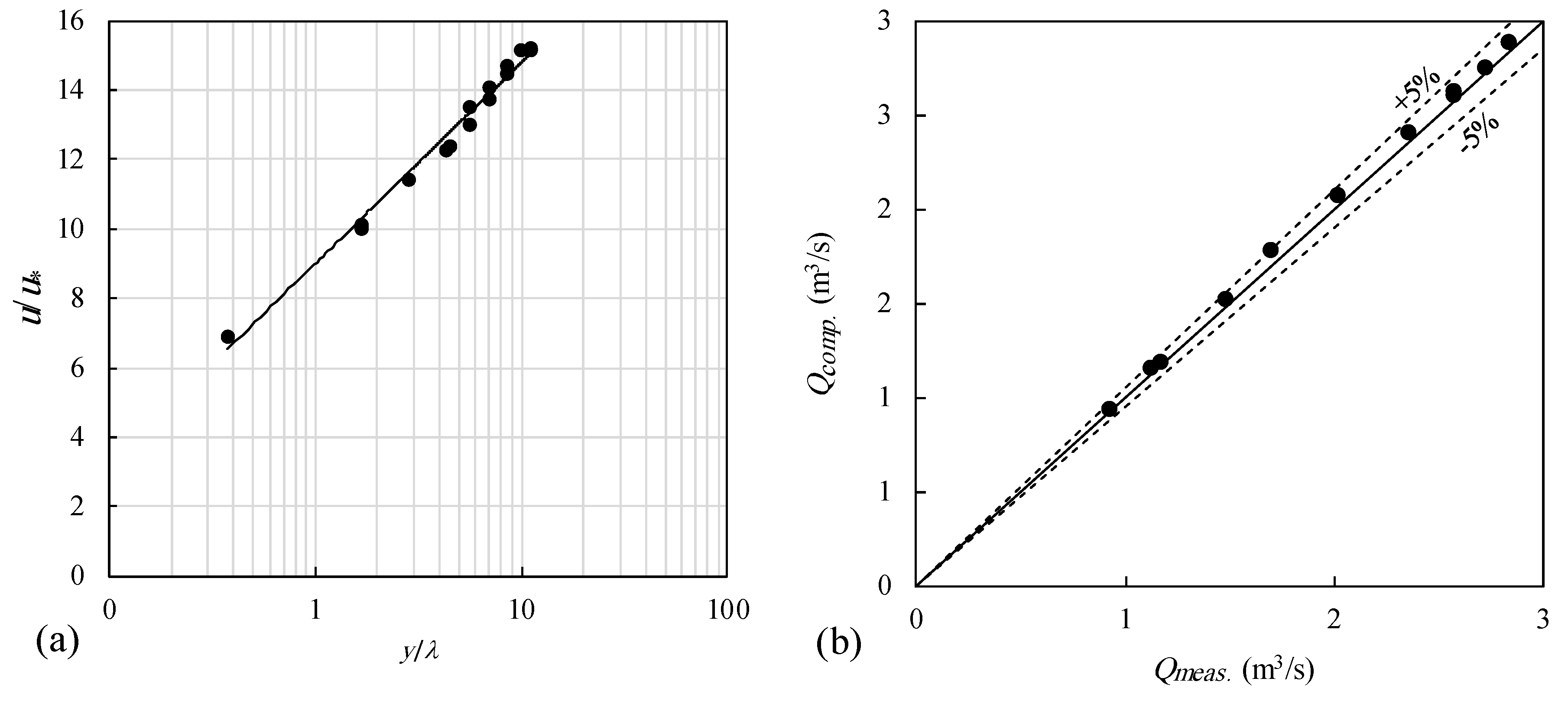
The second part of the experiments deals with the local flow velocity measurement. For two pipe slopes (i = 1.5% and 7.0%), four tests were carried out with h/D of around 0.50 and 0.75 (see Table 1). The velocity profiles were measured utilizing a Pitot-Prandtl tube along the vertical (or centreline) as well as radial directions forming angles of π/8, π/4, 3/8π (22.5°, 45°, 67.5°) with the vertical. The employed Pitot-Prandtl tube was 4 mm in diameter and 60 mm long. It was operated from the above, through one of the observation ports located at a distance of 10.5 m from the pipe inlet. To allow for measurement operations along the transects, it was connected to a digital gauge and to a digital goniometer. The inlet point of the Pitot-Prandtl tube was turned upstream, while its body with the pressure taps was kept parallel to the pipe bottom. The first measurement point was set at the middle of the corrugation crest, at a distance of 3 mm. The static and dynamic pressure data was obtained in turn by the same pressure transducer and data acquisition system with 50 Hz frequency in 30 s durations. The results were compared to those obtained from higher frequencies showing no significant differences. The time-averaged local flow velocity: resulted from taking an average from instantaneous total head minus static head: Δ. Assuming an error of 1 mm on Δ, one may consider the error of around 2.5% for u = 0.5 m/s and of the order of 0.5% for u = 1.5 m/s.
2.2. Discharge Computational Model
The proposed model takes into account water depth h and pipe slope i to predict the flow rate through the following procedure:
- Calculate the average shear velocity and the average roughness Reynolds number , being the water kinematic viscosity;
- Compute “pressurised” flow velocity profile by means of a simple power function with the following form (see Reference [9]):where α and β are the coefficient and the exponent of the velocity power function, respectively. The results analysis by Calomino et al. [9] clarified that both the coefficient α and the exponent β decrease with the discharge or with R*, and they are well expressed by the following two equations for the pipe used in the present study:
- Integrate the velocity profile across the flow cross-section for two schemes of h ≤ r0 and h > r0: where r0 = D/2.
2.2.1. h ≤ r0
Let it be r = r0 − y (see Figure 3a) and , so the element area, dA, is expressed as follows, dr being the element radius:
Assuming that the velocity distribution is the same as in the pressurized pipe flow and by integration within the extremes r = r0 − h and r = r0, one can derive:
The value of Q can be obtained from Equation (4) through the numerical integration.
2.2.2. h > r0
Let it be a = 2r0 − h.
The flow is computed as the difference between a first part, Q1, as in pressurised flow concerning the whole pipe, minus a second part, Q2, concerning the upper circle segment of height a. Q1 can be estimated by integrating over the circle of radius r0, by means of the following equation:
The value of can be derived from the water depth h as shown in Reference [9]; Q2 is obtained with the same formulation of Section 2.2.1 with the value of derived also from the water depth, but considering the distance a instead of water depth h.
2.3. Numerical Model
Recently, the researchers’ interest includes experimental observations as well as a numerical simulation of flow in corrugated pipes. A review of numerical techniques used in this field is given in Reference [4]. Those Authors also presented the details of the numerical simulation of the pressurised pipe flow by means of Large Eddy Simulation (LES) for the 171 mm diameter pipe. In contrast, the simulation of the free-surface flow in corrugated pipes is rare in the literature, especially when the channel slope must be taken into consideration.
In the present study, the flow field is simulated by solving the three-dimensional Reynolds-Averaged Navier-Stokes (RANS) equations (Reference [10], among others) in conservative form as written here in Cartesian coordinates (the fluid is assumed as incompressible and viscous, and the Einstein summation convention is applied to repeated indexes: i, j = 1, 2, 3):
where is the fluid density, the water dynamic viscosity, and the mean fluid pressure, (i = 1, 2, 3) stand for the Cartesian coordinates, denote the mean components of the velocity, and t and are, respectively, the time and the mean strain-rate tensor defined by
The quantity is the Reynolds-stress tensor. The Reynolds-stresses are components of a symmetric second-order tensor. The diagonal components are normal stresses, whereas the off-diagonal elements are shear stresses. Hence, the Reynolds averaging formulation introduces six new unknown quantities that are the six independent components of the symmetric tensor without additional equations. This means that the defined system is undetermined. To close the system, the Boussinesq approximation was used [11]. The kinematic eddy-viscosity has been expressed as a function of the turbulent kinetic energy k and the dissipation rate ω (Equation (9)), leading to a ‘two-equation’ turbulence model.
2.3.1. Two-Equation Turbulence Models
Two-equation models [10] provide one equation to compute the turbulent kinetic energy per unit mass k and one more equation to calculate a specific dissipation rate ω. In fact, two-equation models are complete to predict properties of a given turbulent flow without prior knowledge of the turbulence structure [11]. In the present study, in order to constitute a relationship between the Reynolds stresses and the mean flow field and solve the closure problem, the k-ω model proposed by Wilcox [11] and k-ω SST model developed by Menter [12] were used.
In the k-ω model, the viscosity term is defined as
while the turbulence kinetic energy per unit mass k and the dissipation rate ω obey the following:
In the above equation, ; ; , whereas, and are computed through auxiliary functions as presented in Wilcox [11].
The second selected turbulence model, the k-ω SST [12], has several relatively minor variations from the original SST version [13,14]. The turbulence kinetic energy and the dissipation rate are computed using
where represents a production limiter used in the model to prevent the build-up of turbulence in stagnation regions [12], represents the blending function, defined as [13,14] follows:
with and y represents the distance to the nearest wall. The turbulent eddy viscosity is
where [15], S is defined as the second invariant of the deviatoric stress tensor and . is a second blending function [13,14] expressed as
All the constants are predicted through a blend from the corresponding constants. For example, is calculated as . This model contains the following closure coefficients: ; ; ; ; ; ; [12].
It is to be noted here that the choice of two k-ω type of turbulence models for this work is due to their generally superior performance with respect to the more classical two-equation k-ε model in wall-bounded flows and, in particular, to their suitability in complex boundary layer flows under adverse pressure gradient and separation, as reported in Menter et al. [12].
2.3.2. Numerical Solution
In the four open-channel experimental tests where the velocity was measured, the flow field was simulated by solving the RANS equations with both the k-ω and k-ω SST closure models. The governing Equations (6) and (7), together with the equations of turbulence models, were solved numerically by means of the interFoam solver that is embedded in the OpenFoam® C++ libraries. The interFoam solver has been designed for incompressible, isothermal, immiscible fluids using the VoF (Volume of Fluid) phase -fraction based interface capturing approach [16]. The VoF method was used in many investigations (see References [17,18,19,20], among others). The VoF method, proposed by Hirt and Nichols [17], locates and tracks the free surface flow. In this method, each fluid phase (herein air and water) has an individual fraction of the volume. If a cell is totally void of water but full of air, the magnitude of volume fraction function is assigned to 0; however, when the cell is completely full of water, the aforementioned magnitude is equal to 1. Note that, if the interface intercepts the cell, the function will have a value between 0 and 1. Then, the indicator function, , is expressed as
The two-phase flow can be assumed as a mixed fluid; hence, the density and dynamic viscosity are defined as
in which the subscripts 1 and 2 stand for the two selected fluids [21].
The volume fraction function can be calculated by solving an advection equation for the velocity vector field, V, as follows [17,21]:
The governing equations are discretised with the Finite Volumes (FVM) (see References [21,22,23], among others). As to the discretisation of the solution domain, a ‘structured’ mesh was built where the dependent variables are stored at the cell centre of each cell space domain in a ‘co-located’ arrangement.
In the present study, the PISO (Pressure Implicit with Split Operator) technique suggested by Issa [24] was employed to couple the pressure–velocity in transient computations. The PISO procedure adopts the ‘Segregated Approach’ and the system of equations is solved sequentially [24]. Further details of the transient solution procedure can be found in Reference [23]. The stability of the solution procedure was ensured utilizing an adaptive time step with an initial value of 10−6 s in conjunction with a mean Courant-Friedrichs-Lewy (CFL) number limit set to 0.5.
As shown in Figure 4, a three-dimensional computational grid was generated with an internal diameter D = 0.171 m, a length L = 4 m, a roughness height ε = 0.006 m, and a longitudinal spacing of the roughness elements λ = 0.0254 m. Experimental conditions and fluids properties used in the simulations are presented in Table 1 and Table 2, respectively.
A number of preliminary simulations were performed before selecting the final configuration of the grids. The features of these simulations (that is, A, B, and C) are outlined in Table 3: Δxi are the approximated grid spacing in xi direction, whereas Ntotal is the total number of grid points.
The final three-dimensional finite-volume computational domain includes about 27.5 × 10⁶ grid points, with a grid spacing of approximately 1 mm. The computational domain has been rotated around the x2 axis in order to obtain the longitudinal pipe slope of each test with the rotation matrix:
where is the relevant angle of rotation.
For each simulation, the boundary conditions of no-slip and zero wall-normal velocity at the pipe wall were imposed. On the x1-x3 lateral boundary plane that represents the longitudinal section of the halfpipe, a symmetry boundary condition was set [25]. At the x2-x3 inlet section, the flow depth and discharge values corresponding to the simulated test were applied. As for the x2-x3 outlet cross-section, the gradient of flow velocity was set to zero in the direction perpendicular to the boundary and a fixed value was imposed to pressure, while the free-surface condition was enforced at the flow free surface.
At the beginning of each simulation, the pipe was initially empty and the flow was entered through the pipe inlet. Simulations were run until a steady-state uniform flow condition was achieved.
A CPU based computational system was used to carry out the computations of the present study. The system included 3 Worker Nodes, each one equipped with 4 CPU type E5-2640 (total 96 cores/16 threads @ 2.0 GHz), 128 GB RAM, 1899 MHz, and 1 TB disk space. The simulations were conducted using 16 processors through the public domain openMPI implementation of the standard Message Passing Interface (MPI) for the parallel running. The technique of parallel computing has been adopted as domain decomposition to split the geometry and the associated fields into segments. In this study, the ‘simple geometric decomposition’ technique was used, in which the domain is broken into segments by direction. The computational time was about 240 h CPU time for each simulation.
3. Results and Discussion
3.1. Experimental Results
3.1.1. Stage-Discharge Curves
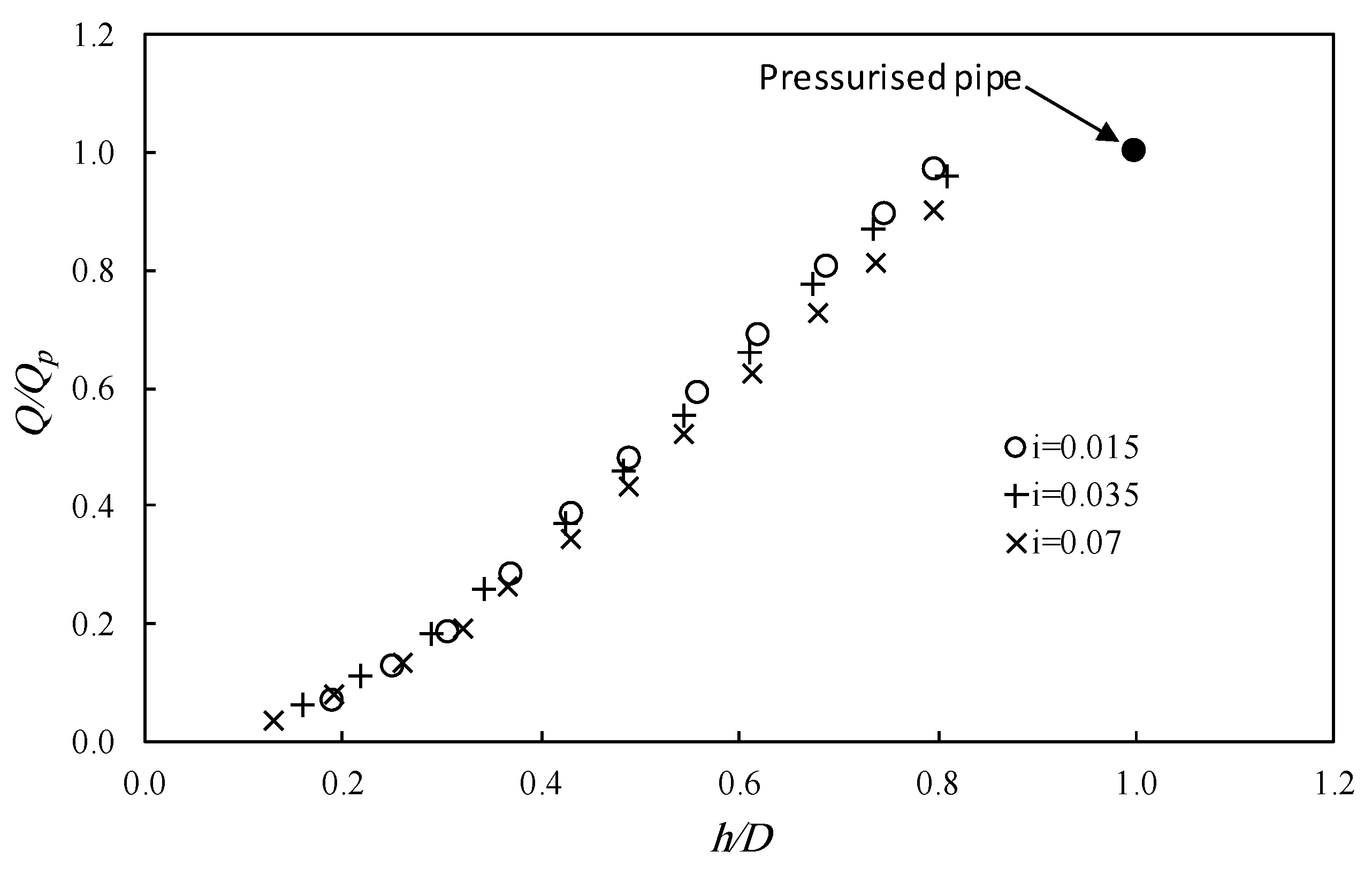
The measured discharges and flow depths are summarised in Figure 5 for the three tested pipe slopes: i = 1.5, 3.5, and 7%. In this figure, the discharge data were normalised by the pressurised pipe flow rate QP, and water depths were made non-dimensional by the minimum internal pipe diameter D = 171 mm. As one can observe, the normalised stage-discharge values for i = 7% are sensibly lower than what resulted for the other two smaller slopes. This is different from what occurs in a fully turbulent flow regime since the Manning coefficients vary with the slope [7].
3.1.2. Friction Factors
If we consider the experimental values of the friction factors, we can represent them in the form of the well-known Moody diagram by means of some curves with identical relative roughness: λ/(2Rh), where Rh is the hydraulic radius, as shown in Figure 6.
In this figure, the Reynolds number and friction factor are, respectively, Re = 4RhU/ν, and f = 8giRh/U2, where g is the gravitational acceleration. It is clear that the curves of the friction factor for the free-surface pipe flow (dashed lines) are generally above the pressurised pipe flow curve (solid line), while under a free-surface flow, the relative roughness can be smaller than in the pressurised condition. It seems that the relative roughness parameter, defined by Morris [1], does not properly identify the roughness role under the free-surface flow condition. As noted in the Introduction, Morris [1] derived his equations for full pipes or wide open-channel flows, where the flow is practically 2D. Figure 6 also depicts that a larger friction factor is expected for a smaller flow depth.
3.1.3. Velocity Profiles
The velocity profiles along the radial directions are shown in Figure 7. The velocity values were made non-dimensional by means of the average shear velocity . Figure 7 contains the profiles (solid lines) computed by the power function (Equation (1)), introducing the value of in it for the selected free-surface test. As to the points above the mid pipe, the distances from the wall were taken from the nearest wall. This method resulted in velocity profiles close enough to the experimental data points.
One can note that the velocity along the centreline was properly simulated by the power function until it decreases owing to the ‘dip phenomenon’. Along the other radial directions, the velocity profile tends to follow the same velocity pattern along the centreline, even though with smaller values. In general, the power function profile may be considered as an average velocity profile for free-surface flow conditions with an acceptable deviation (mainly overestimation) with respect to the experimental values.
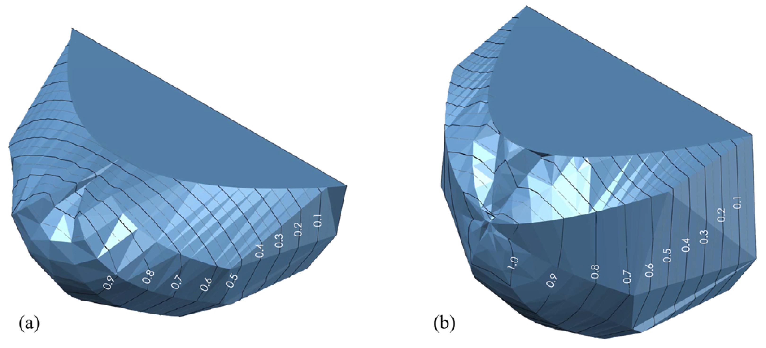
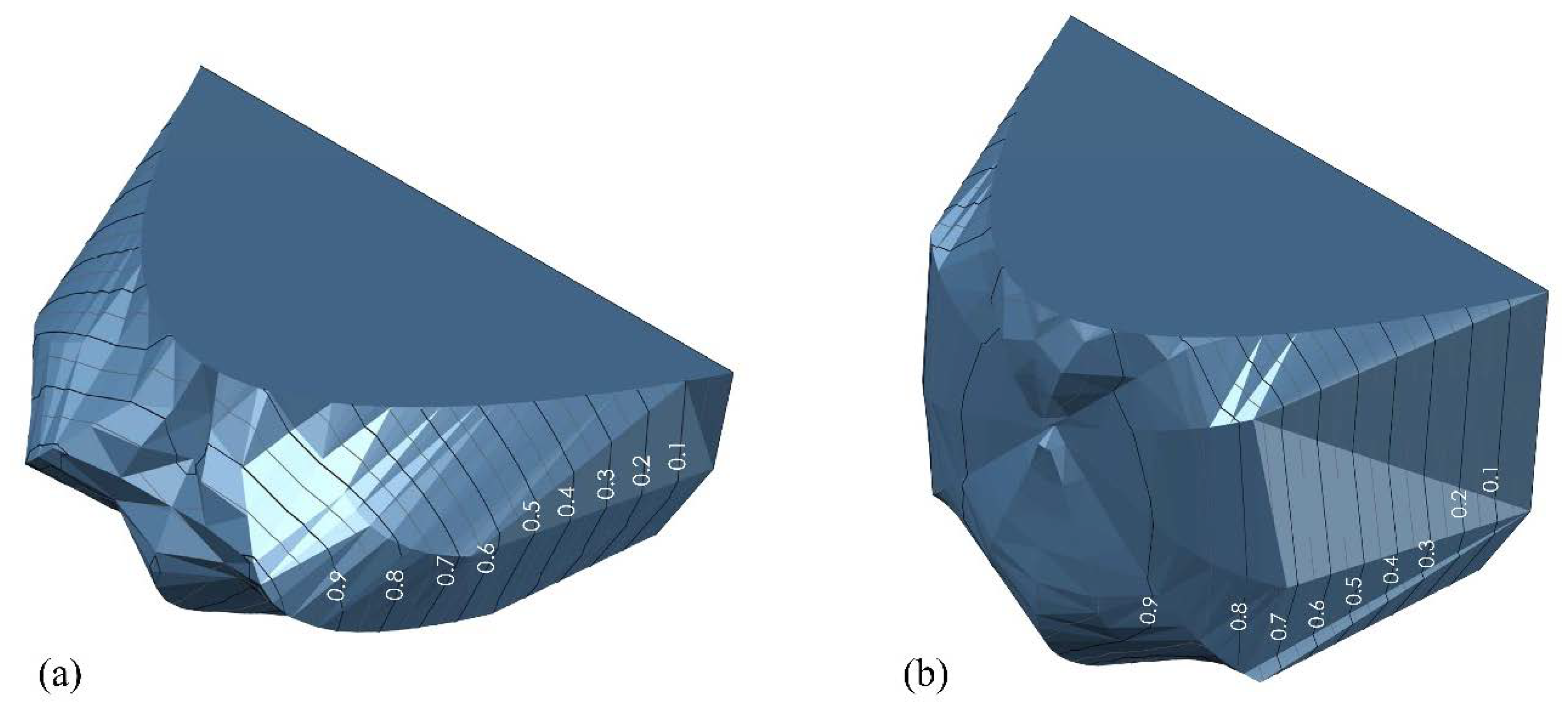
Figure 8 illustrates contours of the flow isovelocity on a 3D representation of the measured longitudinal flow velocity for Tests 1 and 2. To obtain the 3D velocity pattern, the polar coordinates of each velocity data point were transformed into Cartesian coordinates. A polynomial curve was fitted to the velocity data along the pipe centreline in order to estimate the velocity value at the free surface, where a parabolic distribution of velocity has been assumed. To get a smoothed 3D model, a 3rd order polynomial function was fitted to the velocity data of each transect. Ultimately, the polynomial curves were transformed into splines. An application of a 3D velocity model is to estimate the bulk mean flow velocity or the flow rate conveying through the pipe directly from the measured velocity data points. The developed 3D models of the present study predict flow discharges of 7.10 and 12.78 L/s for Tests 1 and 2. These values are 9.9% and 12% smaller than the corresponding observed ones (see Table 1). The relatively small number of the measured velocity points with respect to the entire flow cross-sectional area is a cause of the resulted prediction error.
3.2. Evaluation of the Discharge Computation Model
The developed model in Section 2.2 is evaluated herein using the experimental data of the present study (that is, the University of Calabria dataset) and three other literature datasets.
3.2.1. University of Calabria Dataset
Table 4 furnishes the predicted discharge for the pipe slopes 1.5% and 7.0%. For these four tests, the velocity profiles are available (see Table 1). This Table clarifies that the model prediction error is less than 15%. The percent prediction error e was calculated as
where Qcomp. and Qmeas. are the computed and measured flow discharges.
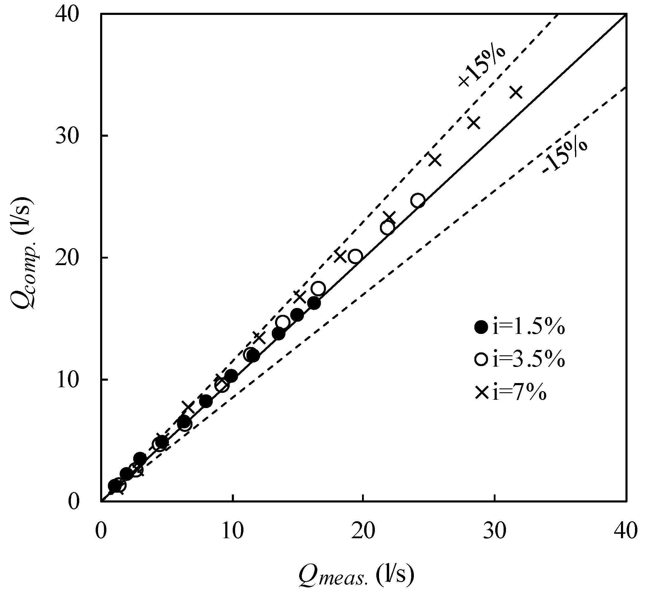
Moreover, the 34 tests on the discharge measurement with the slopes 1.5%, 3.5%, and 7.0% were, in turn, simulated. The maximum and minimum values of the model prediction error are as follows: for i = 1.5%, emax = 11.7% and emin = −0.47%; for i = 3.5%, emax = 4.1% and emin = −15.2%; and, for i = 7%, emax = 15.1% and emin = −12.0%. Figure 9 illustrates the computed and measured flow discharges along with the lines representing the ±15% deviations, where most of the computed values lay in.
Obviously, the proposed analytical model contains two sources of error. First, the velocity profile in a pressurised pipe is not exactly the same as what occurs in a pipe under free-surface flow conditions; indeed, in the pressurised pipe, the flow is symmetric with respect to the section centre, while in free-surface flow, it is symmetric with respect to the section axis perpendicular to the pipe bottom. Second, the model does not take into account the dip phenomenon along the velocity profiles. Therefore, the identified flow velocity for the model is larger than the real values near the water surface; this may lead to slight over-predictions for larger pipe slopes. Considering the uncertainties in velocity, water depth, and discharge measurement, apart from the model assumptions, such results are acceptable.
3.2.2. Webster and Metcalf Dataset [5]
Webster and Metcalf presented results of 11 tests under free-surface pipe flow in a 150.9 cm corrugated pipe. To assess the proposed model by using this dataset, Equation (24) was used to numerically integrate the velocity across the flow section:
This equation was obtained from the velocity data of a test made by Webster and Metcalf [5] under the pressurised flow condition (Figure 10a). The von Kármán κ and the constant are 0.397 and 9.0, respectively: these values are close to those usually assumed for rough turbulent flow. It is interesting to note that choosing the corrugation height ε as the length scale instead of the spacing λ will not change the slope of the regression line, but only the constant value.
The results (Figure 10b) show small over-predictions of the measured discharge values, with the maximum and minimum deviations equal to 4.18% and −0.35% respectively; the maximum deviations are associated with the flow depths of around D/2.
3.2.3. Ead et al. Dataset [6]
Ead et al. did not take any velocity measurement under the pressurised pipe flow condition; nevertheless, the computational model was run on the basis of the centreline velocity profile equation adopted by Ead et al. as follows
where is the local shear velocity and the distance yo is computed starting from 6 mm below the roughness crest. The proposed flow model herein was used to integrate the velocity profiles across the flow area. Figure 11 shows that the model prediction error is independent of the pipe slope, with a maximum of 18% for h = 0.12 m and i = 1.4%. Small pipe slopes in the Ead et al. tests (less than 2.6%) could be a reason for the independence of the model errors from the pipe slopes.
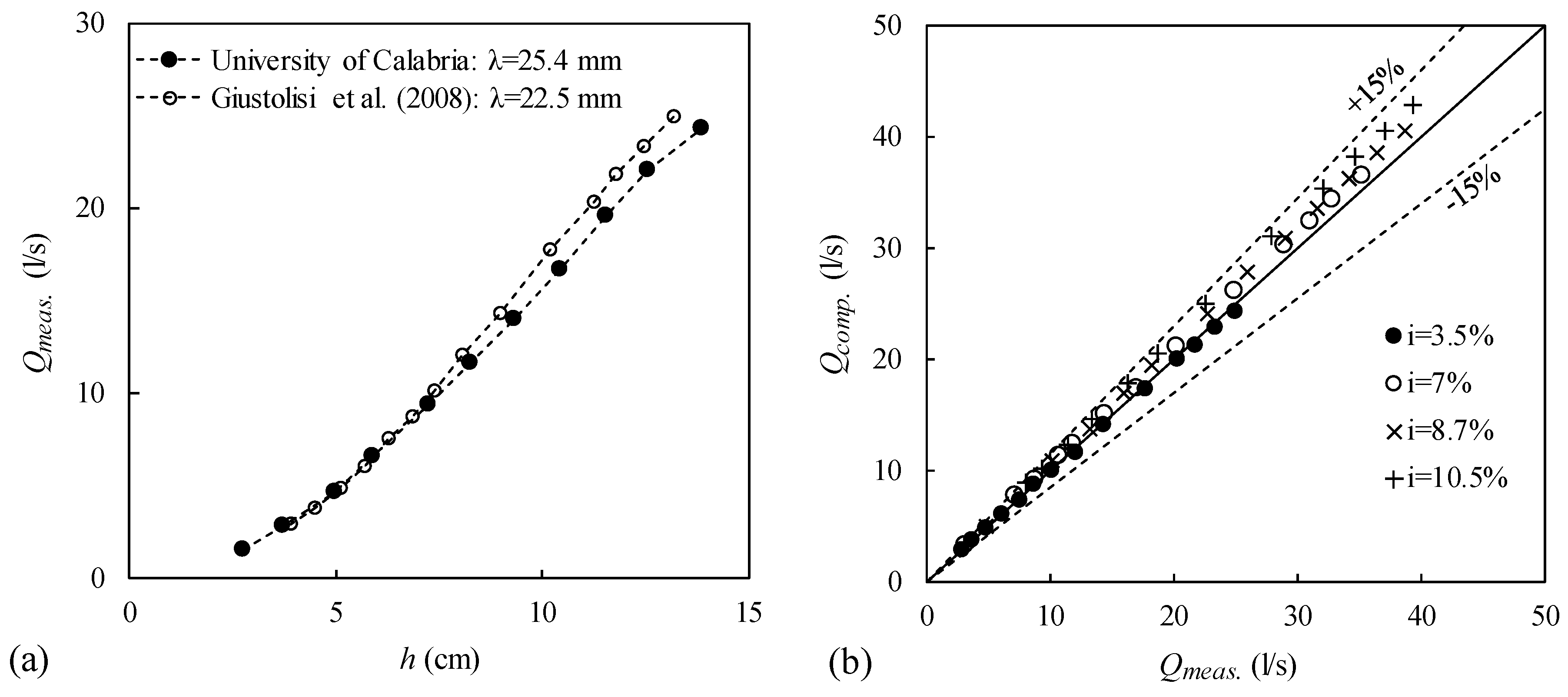
3.2.4. Giustolisi et al. Dataset [7]
Giustolisi et al. carried out free-surface flow tests without taking any velocity measurements. The 171 mm pipe tested by those authors is somewhat different from the one used at the University of Calabria, although the pipe producer was the same. Indeed, the roughness spacing λ was 22.5 mm in Giustolisi et al. [7], whereas it was 25.4 mm in the pipe tested in the present study. Comparing the stage-discharge curve of the University of Calabria dataset with that obtained from the Giustolisi et al. data for the slope 3.5%, as presented in Figure 12a, clarifies that the curve resulted from the University of Calabria data lies under the one observed by the aforementioned authors; indeed, this effect is coherent with the pipe resistance, which increases, according to Morris [1], with the roughness spacing λ for a wake-interference flow.
Figure 12b presents the predicted discharge results for the Giustolisi et al. dataset [7], utilizing the proposed flow computation model, along with the velocity profile equation (Equations (1) and (2)). It is evident that the simulated discharges match well enough with the experimental ones, even though they appear to be overestimated as the pipe slope and water depth increase.
3.3. Numerical Simulation Results
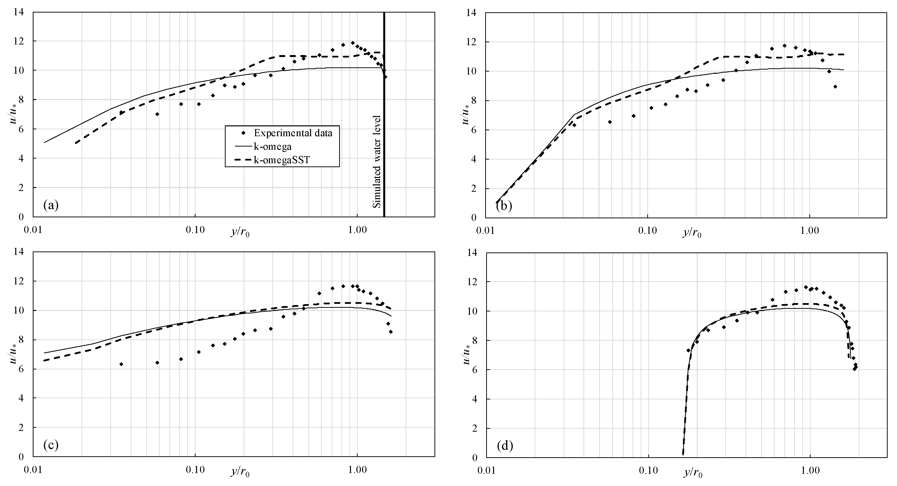
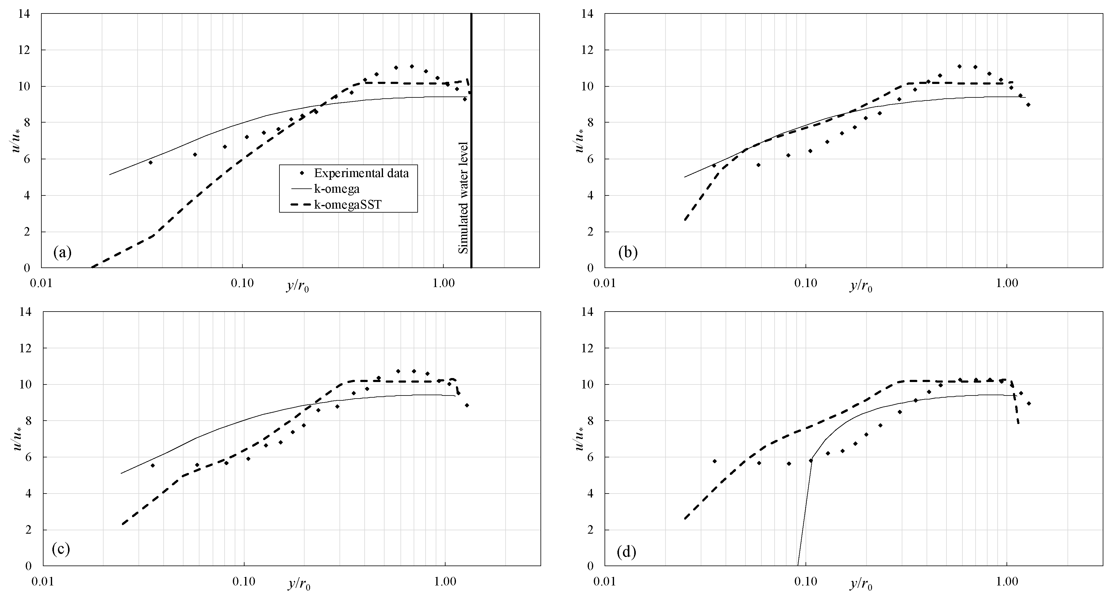
From Figure 13, Figure 14, Figure 15 and Figure 16, one can find the normalized experimental velocity profiles versus y/r along with the simulated profiles. The computed profiles in the flow core zone are more uniform than the observed ones and the ‘velocity dip’, if present, is limited to a narrow band near the water surface. The velocity values computed by the k-ω model are, in general, smaller than those computed by the k-ω SST model. However, the profiles simulated by both models can be considered satisfactory when compared with the experimental points. In particular, if one looks at Figure 13, Figure 14, Figure 15 and Figure 16, in the portions of the figures in which the experimental datasets are available, the latter are satisfactorily reproduced in some cases by one model, in other cases by the other model, in some other cases (many of them) by both. This means in the first place that the k-ω class of models can be used by all means in this type of problems for engineering purposes. Moreover, the differences between experiments and numerical data are well in the ranges usually encountered in using models of turbulence. A more accurate correspondence between the experiments and calculations could be obtained only by changing the approach, that is, using Direct Numerical Simulation of turbulence instead of modelling, but this would require enormous computing resources, and also, it would be a physics-of-fluids study no more, instead, an engineering one.
Figure 17 illustrates the 3D representation of the simulated longitudinal velocity as well as the simulated flow velocity contours using k-ω SST model for Tests 1 and 2. The general velocity pattern and contours of the flow velocity are similar to what was previously obtained from the experimental data (see Figure 8).
Table 5 furnishes a comparison between the numerical and experimental discharge values: Qnum. and Qexp. The latter values were the sum of fluxes through each cell in the cross-section where the velocity magnitudes were simulated. The table shows that the deviations are of small magnitudes in any case. Similarly, the comparison between the simulated and measured water depths (that is, hnum. and hexp.), as presented in Table 6, clarifies that the deviations are also negligible. The simulated water levels of Tests 1 to 4 using the k-ω SST turbulence model are depicted in Figure 13, Figure 14, Figure 15 and Figure 16.
Figure 18 shows the velocity vectors in one of the pipe cross-sections; in the bulk of flow, the prevailing velocity direction is streamwise, whereas, near the pipe wall, stronger spanwise velocity components appear. In general, the secondary circulation is relatively weak, with vector magnitude of the order of no more than 1/10 of the streamwise component. In Figure 18, a solid line representing the corrugation crest is also depicted. In some points, the transverse velocity vectors appear to cross this line, owing to the vector scale. In reality, the tails of these vectors lay at 0.5 to 1 mm from the wall. It should be noted that the present study was mainly conducted aiming at the prediction of flow discharge and water level, and those results are rather satisfactory. The study of ‘secondary flows’ needs a more detailed step in the research, a much more physics-oriented approach rather than an engineering-oriented one.
Figure 19 shows a longitudinal section of the pipe, including the velocity vectors within the corrugation trough, where the recirculation region is obvious. Above this zone, a very weak layer with velocity direction towards the end of the corrugation trough occurs. The existence of this zone amplifies the idea that the space inside the corrugation may not contribute much to the flow conveyance.
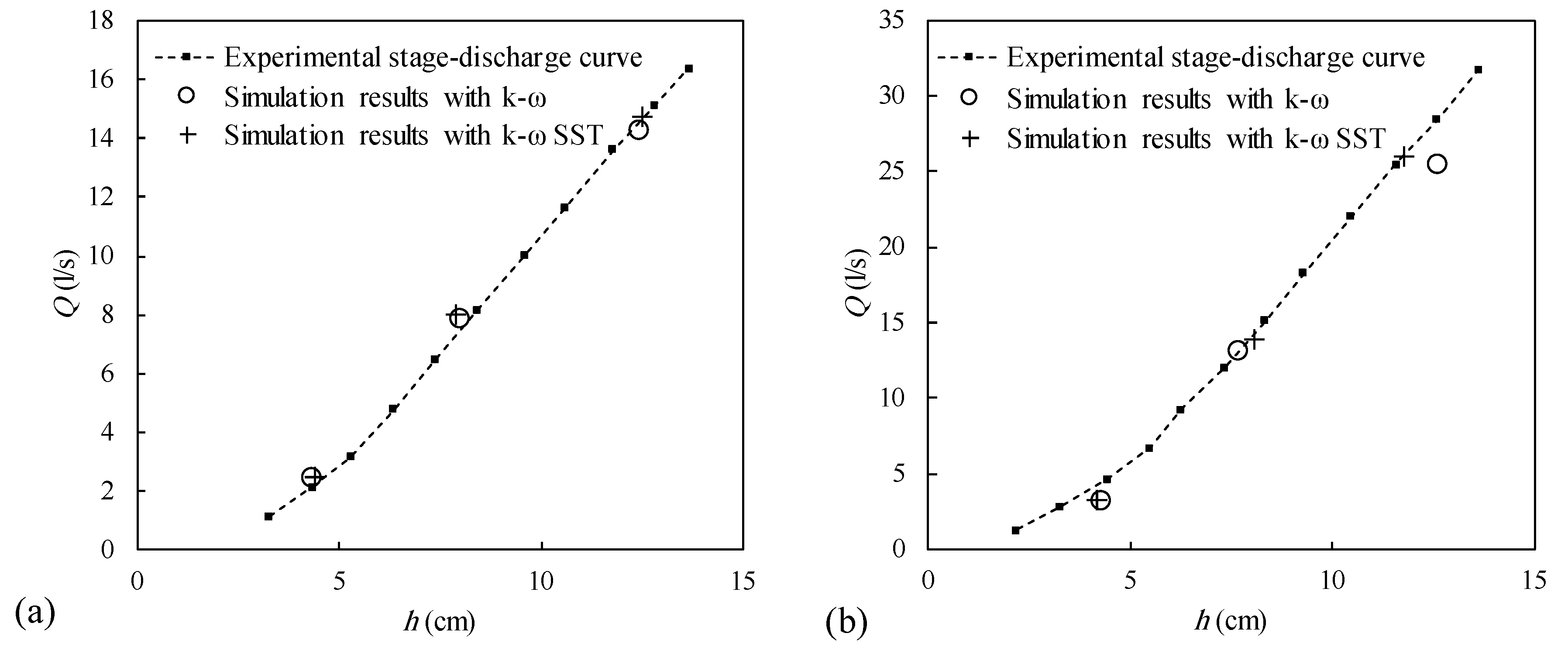
In addition to the four tests with the observed velocities, two more simulations (that is, Tests no. 5 and 6) were carried out with h/D = 0.25 and the pipe slopes i = 1.5% and i = 7%, respectively. The results are available in Table 7, depicting very small deviations from the experimental data. The aim of performing these two test was to assess the reliability of the numerical model in the generation of the stage-discharge curve. Figure 20 illustrates a comparison of the numerical simulation results with the stage-discharge curve for two pipe slopes. It is clear that the numerical simulation can be considered as an alternative approach to generating the entire stage-discharge curve without performing laboratory tests. In order to improve the present results, one may increase the spatial resolution of the computing domain or, eventually, use the Large Eddy Simulation (LES) approach for numerical simulation. Both these options require the use of a much more powerful computing system.
4. Conclusions
The experimental results show that the stage-discharge curve of an internally corrugated pipe may vary with the pipe slope. This is probably attributable to the dependency of the pipe hydraulic roughness parameter (for example, Manning’s roughness coefficient) on the pipe slope. Moreover, analysis of the Darcy friction factor revealed that under the free-surface flow condition, larger flow depth may lead to the smaller friction factor, while, for a certain flow depth, the friction factor may increase as the pipe slope increases. Of course, further study is needed to confirm such results for other flow conditions, in particular for a wider range of the Reynolds number.
A simple model based on the velocity profiles observed in the pressurised pipe was developed to compute the pipe flow discharge under the free-surface flow condition. The proposed model was evaluated by means of new experiments as well as three other available literature datasets for the pipe slopes up to 10.5%. This range covers many draining pipe slopes available in the field: according to Dennis [25], land drainage pipes are placed at absolute gradients from 0 to around 8% (0.1% to 5% is a more common range). The results showed that, in general, smaller accuracy is expected for larger flow depths and pipe slopes. Nevertheless, the model offered accurate enough predictions of less than 20% error.
The use of the numerical simulations based on the RANS equations provides a completely different approach, by which good results can be obtained. In this case, the numerical simulations are based only on the Navier–Stokes equations and the pipe wall geometry and do not demand any empirical knowledge. The method looks promising if computational resources are available. Two well-known turbulence models were assessed to predict the flow velocity profiles. Both models gave enough accurate results. The simulated velocity field confirms the existence of recirculation zones within the cavities as well as secondary currents in the cross-sectional plane. The numerical model is also able to predict stage-discharge curve of the pipe flow on the basis of the simulated flow velocity field.
Author Contributions
F.C., R.G., A.D. contributed in the design, performing and result analysis of the laboratory tests; A.T. finalized the paper draft; discharge computation model was developed by F.C.; whereas, G.A. and A.L. carried out the numerical simulations. Analysis of the 3D flow pattern was made by S.A.
Conflicts of Interest
The authors declare no conflict of interest.
References
- Morris, H.M. Flow in rough conduits. Trans. ASCE 1955, 120, 373–410. [Google Scholar]
- Morris, H.M. Design methods for flow in rough conduits. J. Hydraul. Div. 1959, 85, 43–62. [Google Scholar]
- Shipton, R.J.; Graze, H.R. Flow in corrugated pipes. J. Hydraul. Div. 1959, 102, 1343–1351. [Google Scholar]
- Calomino, F.; Tafarojnoruz, A.; De Marchis, M.; Gaudio, R.; Napoli, E. Experimental and numerical study on the flow field and friction factor in a pressurized corrugated pipe. J. Hydraul. Eng. 2015, 141, 04015027. [Google Scholar] [CrossRef]
- Webster, M.J.; Metcalf, L.R. Friction factors in corrugated metal pipes. J. Hydraul. Div. 1959, 85, 35–67. [Google Scholar]
- Ead, S.A.; Rajaratnam, N.; Katopodis, C.; Ade, F. Turbulent open-channel flow in circular corrugated culverts. J. Hydraul. Eng. 2000, 126, 750–757. [Google Scholar] [CrossRef]
- Giustolisi, O.; Doglioni, A.; Laucelli, D. Determination of friction factor for corrugated drains. Water Manag. 2008, 161, 31–42. [Google Scholar] [CrossRef]
- Clark, S.P.; Kehler, N. Turbulent flow characteristics in circular corrugate culverts at mild slopes. J. Hydraul. Res. 2011, 49, 676–684. [Google Scholar] [CrossRef]
- Calomino, F.; D’ Ippolito, A.; Gaudio, R.; Tafarojnoruz, A. Pressurised flow in a corrugated pipe. In Proceedings of the a One-Day Congress on 80th Birthday of Prof. Giuseppe Frega, Università della Calabria, Rende, Italy, 21 December 2015; EdiBios: Cosenza, Italy, 2016; pp. 33–46. [Google Scholar]
- Alfonsi, G. Reynolds-averaged Navier-Stokes equations for turbulence modeling. Appl. Mech. Rev. 2009, 62, 040802. [Google Scholar] [CrossRef]
- Wilcox, D.C. Turbulence Modeling for CFD; DCW Industries Inc.: La Cañada, CA, USA, 1998. [Google Scholar]
- Menter, F.R.; Kuntz, M.; Langtry, R. Ten years of industrial experience with the SST turbulence model. In Proceedings of the 4th International Symposium on Turbulence, Heat and Mass Transfer, Antalya, Turkey, 12–17 October 2003; Begell House Inc.: Danbury, CO, USA, 2003; pp. 625–632. [Google Scholar]
- Menter, F.R. Zonal two-equation k-ω turbulence model for aerodynamics flows. In Proceedings of the 23rd Fluid Dynamics, Plasmadynamics, and Lasers Conference, Orlando, FL, USA, 6–9 July 1993; AIAA Paper 93-2906. The American Institute of Aeronautics and Astronautics (AIAA): Reston, VA, USA, 1993. [Google Scholar]
- Menter, F.R. Two-equation Eddy-Viscosity Turbulence Models for Engineering Applications. AIAA J. 1994, 32, 1598–1605. [Google Scholar] [CrossRef]
- Bodnár, T.; Příhoda, J. Numerical simulation of turbulent free-surface flow in curved channel. Flow Turbul. Combust. 2006, 76, 429–442. [Google Scholar] [CrossRef]
- OpenFOAM® User Guide. Available online: https://cfd.direct/openfoam/user-guide/ (accessed on 10 September 2017).
- Hirt, C.W.; Nichols, B.D. Volume of fluid (VOF) method for the dynamics of free boundaries. J. Comp. Phys. 1981, 39, 201–225. [Google Scholar] [CrossRef]
- Alfonsi, G.; Lauria, A.; Primavera, L. On evaluation of wave forces and runups on cylindrical obstacles. J. Flow Vis. Image Process. 2013, 20, 269–291. [Google Scholar] [CrossRef]
- Alfonsi, G.; Lauria, A.; Primavera, L. The field of flow structures generated by a wave of viscous fluid around vertical circular cylinder piercing the free surface. Procedia Eng. 2015, 116, 103–110. [Google Scholar] [CrossRef]
- Alfonsi, G.; Lauria, A.; Primavera, L. Recent results from analysis of flow structures and energy modes induced by viscous wave around a surface-piercing cylinder. Math. Probl. Eng. 2017, 2017, 5875948. [Google Scholar] [CrossRef]
- Rusche, H. Computational Fluid Dynamics of Dispersed Two-Phase Flows at High Phase Fractions. Ph.D. Thesis, University of London, London, UK, December 2002. [Google Scholar]
- Ferziger, J.H.; Perić, M. Computational Methods for Fluid Dynamics; Springer: Berlin, Germany, 1996. [Google Scholar]
- Jasak, H. Error Analysis and Estimation for the Finite Volume Method with Applications to Fluid Flows. Ph.D. Thesis, Imperial College, London, UK, June 1996. [Google Scholar]
- Issa, R.I. Solution of the implicitly discretised fluid flow equations by operator-splitting. J. Comp. Phys. 1986, 62, 40–65. [Google Scholar] [CrossRef]
- Dennis, C.W. The hydraulic characteristics of plastic land drainage pipe. Proc. Inst. Civ. Eng. 1973, 55, 273–284. [Google Scholar]
Figure 1.
The roughness geometry of the selected pipe in the present study: (a) details of the pipe corrugation; (b) a photo of the roughness elements.
Figure 1.
The roughness geometry of the selected pipe in the present study: (a) details of the pipe corrugation; (b) a photo of the roughness elements.

Figure 2.
(a) The observation ports cut on the top of the corrugated pipe; (b) a close-up view of an observation port.
Figure 2.
(a) The observation ports cut on the top of the corrugated pipe; (b) a close-up view of an observation port.
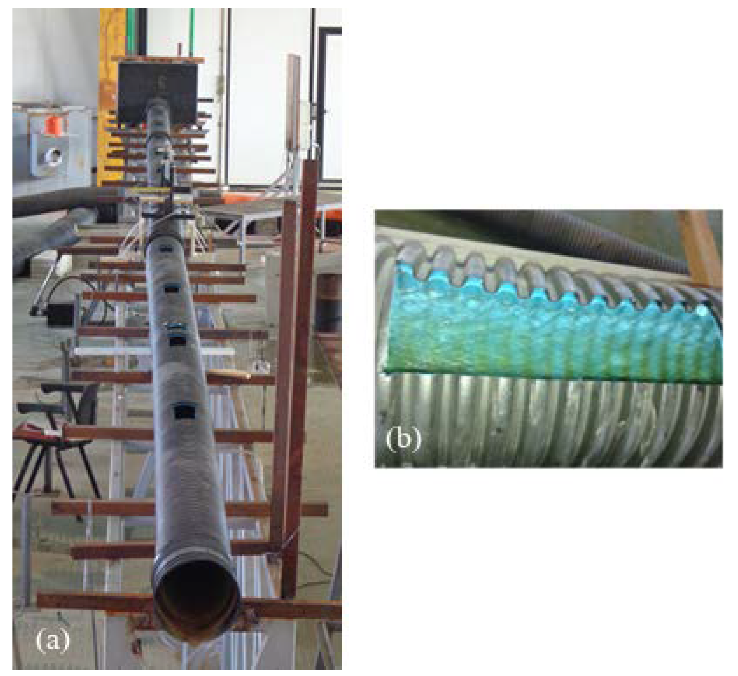
Figure 3.
The configuration of flow and parameters: (a) h ≤ r0; (b) h > r0.
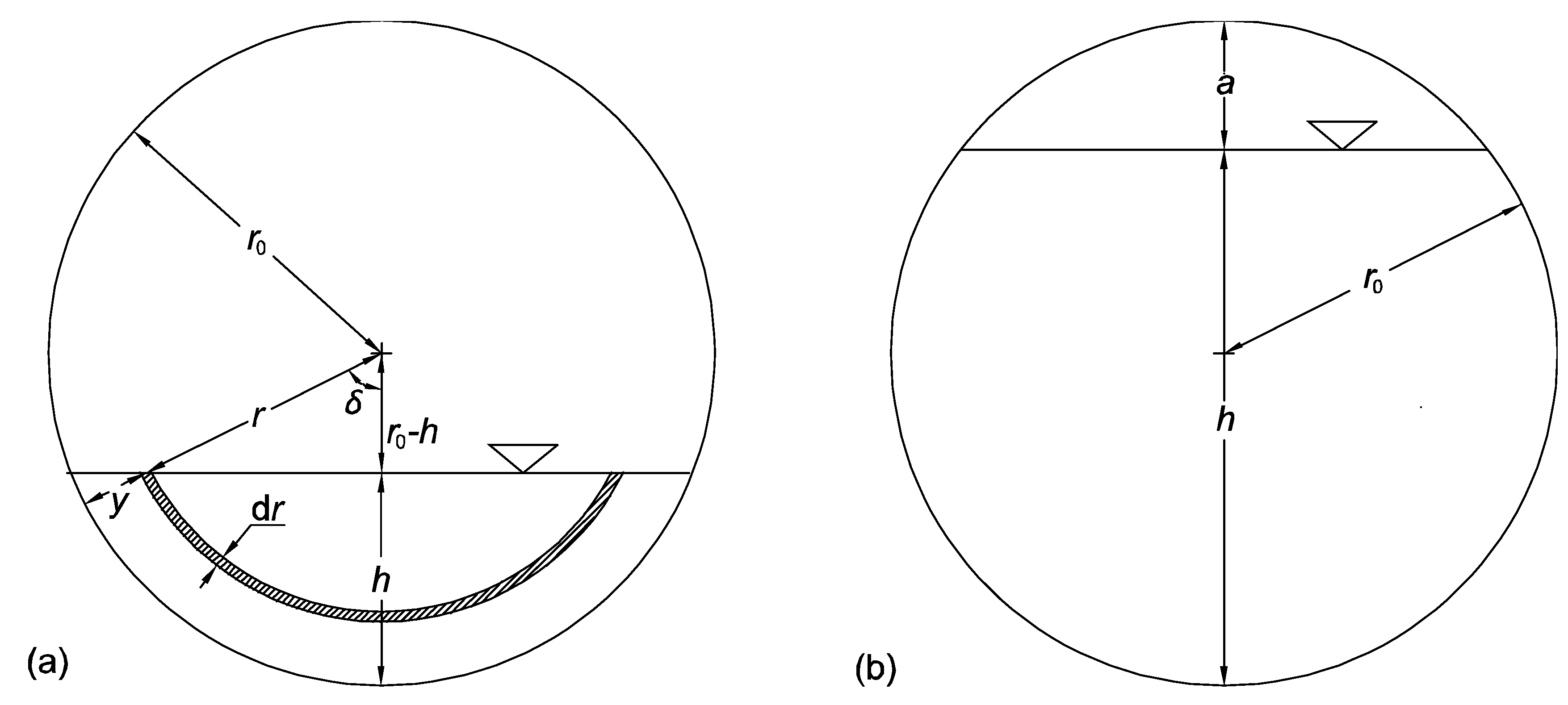
Figure 4.
The computational grid: (a) cross-sectional view of the mesh; (b) longitudinal section of the mesh; (c) 3D representation of the computational grid.
Figure 4.
The computational grid: (a) cross-sectional view of the mesh; (b) longitudinal section of the mesh; (c) 3D representation of the computational grid.
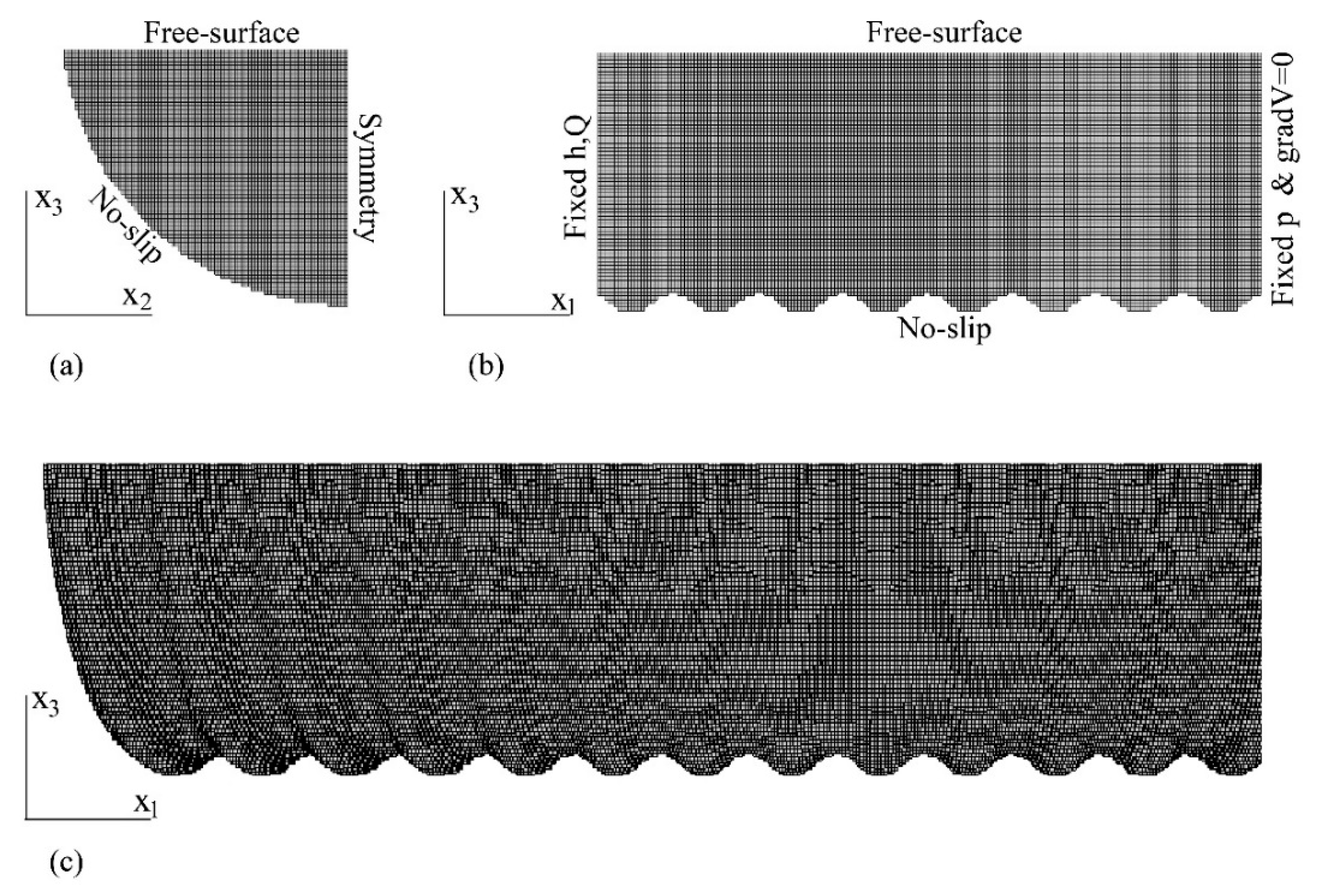
Figure 5.
The stage-discharge data measured at the University of Calabria.

Figure 6.
The behaviour of the friction factor in pressurised and free-surface flow conditions.
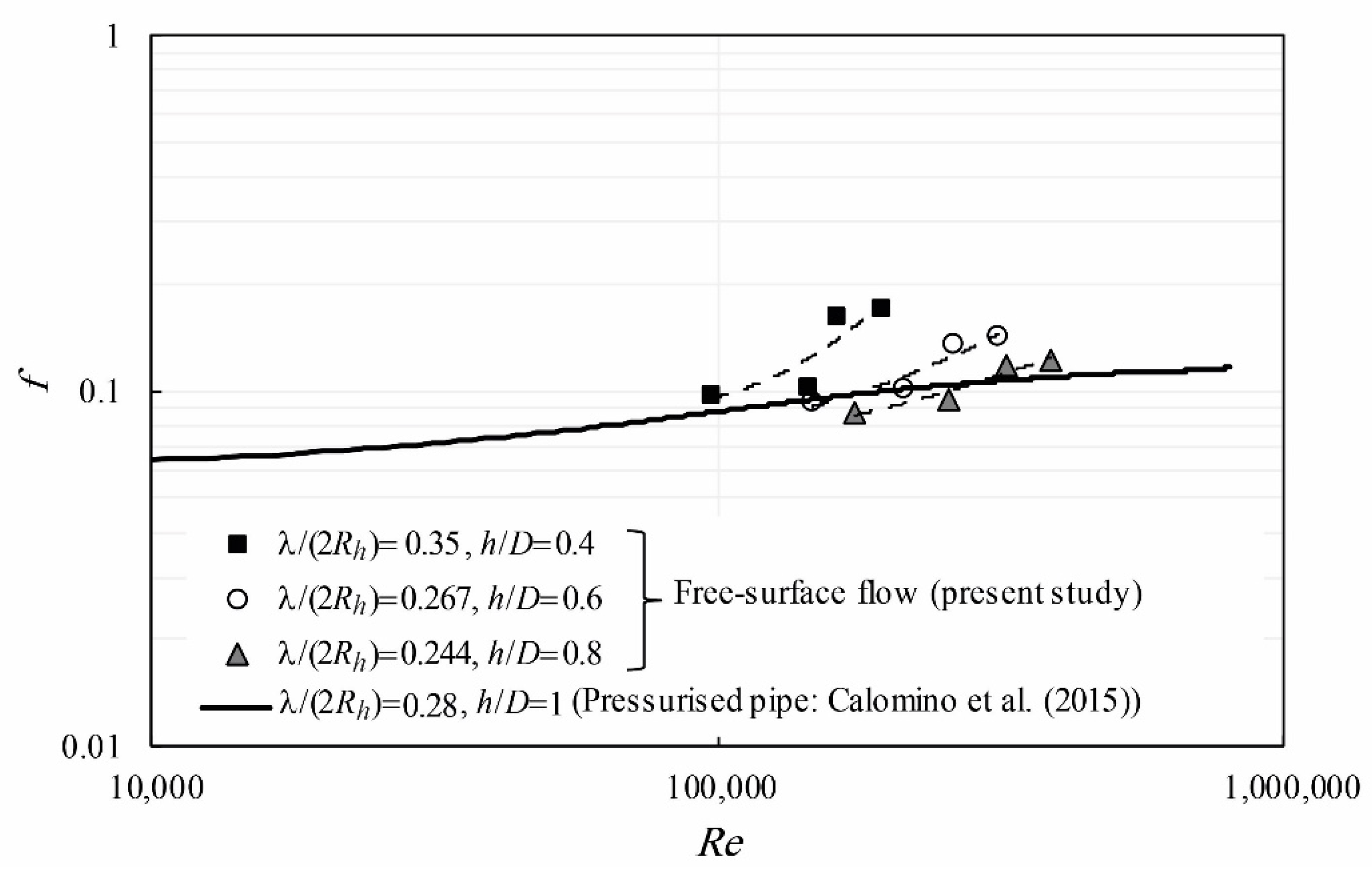
Figure 7.
The velocity distribution along radial directions: (a) Test 1; (b) Test 2; (c) Test 3; (d) Test 4.
Figure 7.
The velocity distribution along radial directions: (a) Test 1; (b) Test 2; (c) Test 3; (d) Test 4.
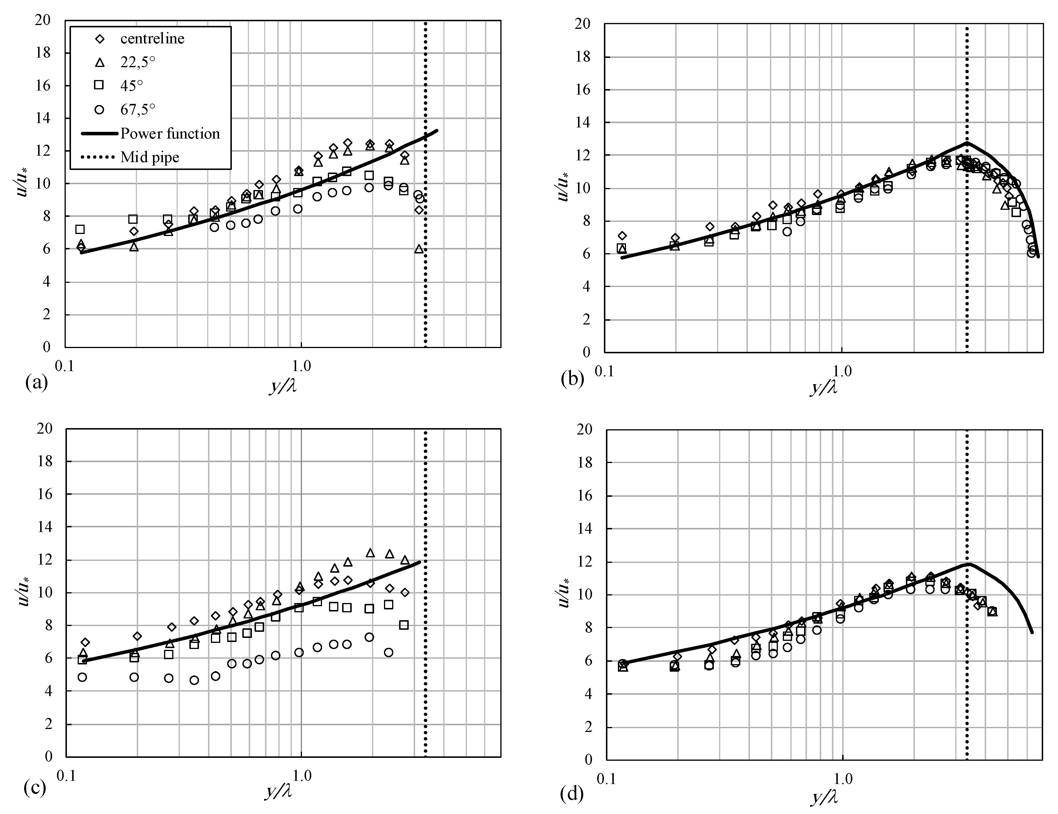
Figure 8.
The contours of the flow isovelocity on the 3D representation of the measured longitudinal flow velocity: (a) Test 1; (b) Test 2 (unit: m/s).
Figure 8.
The contours of the flow isovelocity on the 3D representation of the measured longitudinal flow velocity: (a) Test 1; (b) Test 2 (unit: m/s).

Figure 9.
The measured and computed discharge of the University of Calabria dataset.

Figure 10.
The Webster and Metcalf dataset [5]: (a) the velocity profile of the pressurized pipe flow; (b) the measured versus computed discharges for free-surface flow conditions.
Figure 10.
The Webster and Metcalf dataset [5]: (a) the velocity profile of the pressurized pipe flow; (b) the measured versus computed discharges for free-surface flow conditions.

Figure 11.
The measured and computed discharge of the Ead et al. dataset [6].
Figure 11.
The measured and computed discharge of the Ead et al. dataset [6].

Figure 12.
(a) The stage-discharge curves for i = 3.5%; (b) the measured and computed discharge of the Giustolisi et al. dataset.
Figure 12.
(a) The stage-discharge curves for i = 3.5%; (b) the measured and computed discharge of the Giustolisi et al. dataset.

Figure 13.
The comparison of the experimental velocity profiles with the numerical simulation results for Test 1 along four radial angles from the vertical: (a) 0°; (b) 22.5°; (c) 45°; (d) 67.5°.
Figure 13.
The comparison of the experimental velocity profiles with the numerical simulation results for Test 1 along four radial angles from the vertical: (a) 0°; (b) 22.5°; (c) 45°; (d) 67.5°.
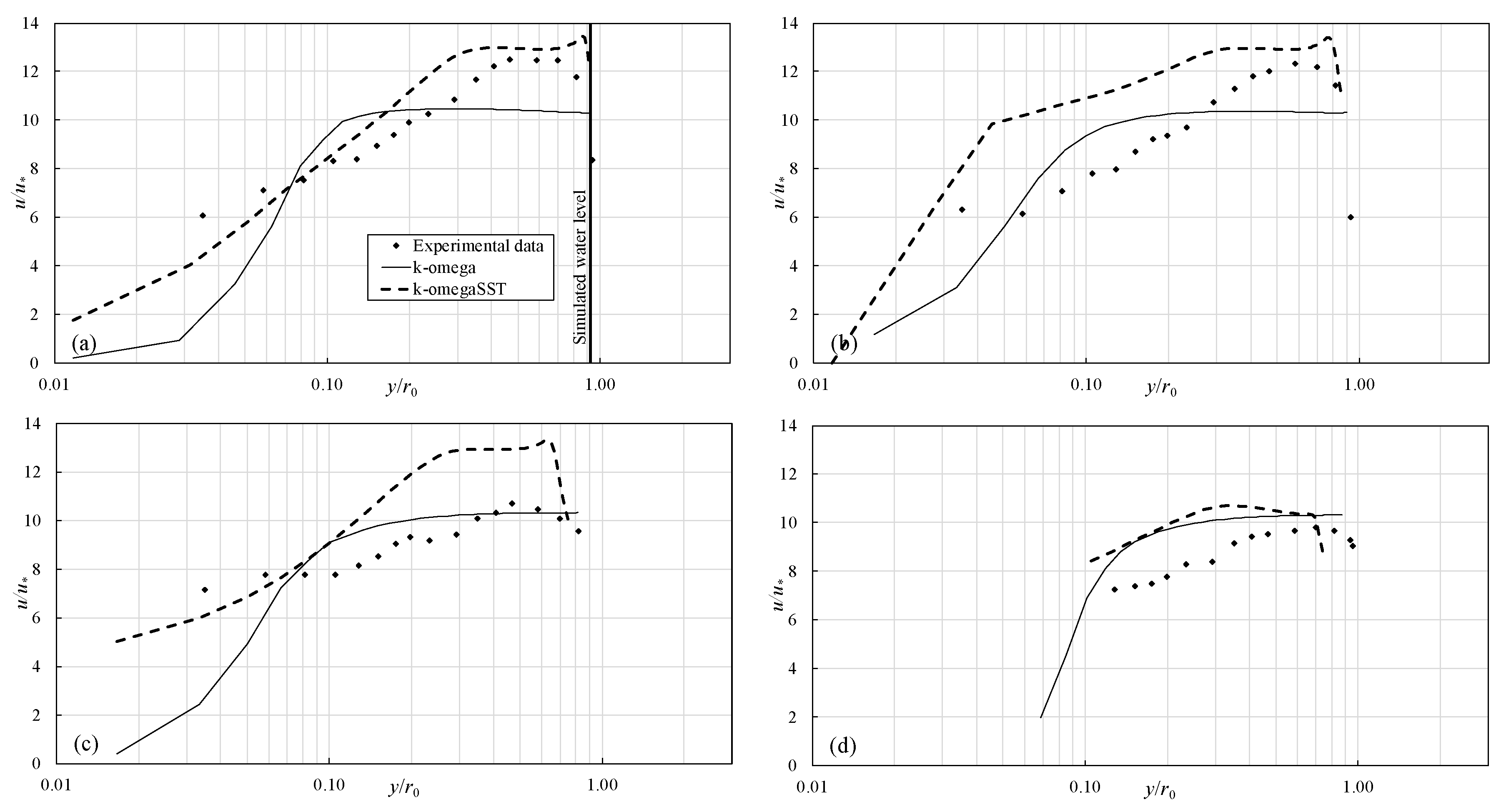
Figure 14.
The comparison of the experimental velocity profiles with the numerical simulation results for Test 2 along four radial angles from the vertical: (a) 0°; (b) 22.5°; (c) 45°; (d) 67.5°.
Figure 14.
The comparison of the experimental velocity profiles with the numerical simulation results for Test 2 along four radial angles from the vertical: (a) 0°; (b) 22.5°; (c) 45°; (d) 67.5°.

Figure 15.
The comparison of the experimental velocity profiles with the numerical simulation results for Test 3 along four radial angles from the vertical: (a) 0°; (b) 22.5°; (c) 45°; (d) 67.5°.
Figure 15.
The comparison of the experimental velocity profiles with the numerical simulation results for Test 3 along four radial angles from the vertical: (a) 0°; (b) 22.5°; (c) 45°; (d) 67.5°.

Figure 16.
The comparison of the experimental velocity profiles with the numerical simulation results for Test 4 along four radial angles from the vertical: (a) 0°; (b) 22.5°; (c) 45°; (d) 67.5°.
Figure 16.
The comparison of the experimental velocity profiles with the numerical simulation results for Test 4 along four radial angles from the vertical: (a) 0°; (b) 22.5°; (c) 45°; (d) 67.5°.

Figure 17.
The contours of the simulated flow velocity on a 3D representation of the simulated longitudinal velocity: (a) Test 1; (b) Test 2 (unit: m/s).
Figure 17.
The contours of the simulated flow velocity on a 3D representation of the simulated longitudinal velocity: (a) Test 1; (b) Test 2 (unit: m/s).

Figure 18.
The simulated velocity vectors in the x2-x3 plane (that is, pipe cross-section) for Test no. 3.
Figure 18.
The simulated velocity vectors in the x2-x3 plane (that is, pipe cross-section) for Test no. 3.
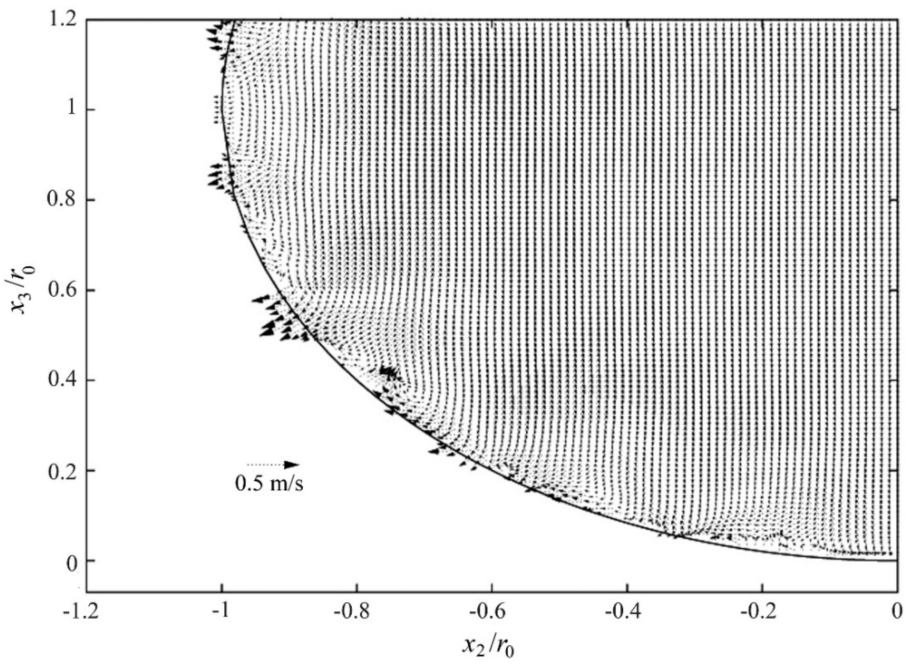
Figure 19.
The longitudinal pipe section with the simulated velocity vectors in the x1-x3 plane for Test no. 3.
Figure 19.
The longitudinal pipe section with the simulated velocity vectors in the x1-x3 plane for Test no. 3.
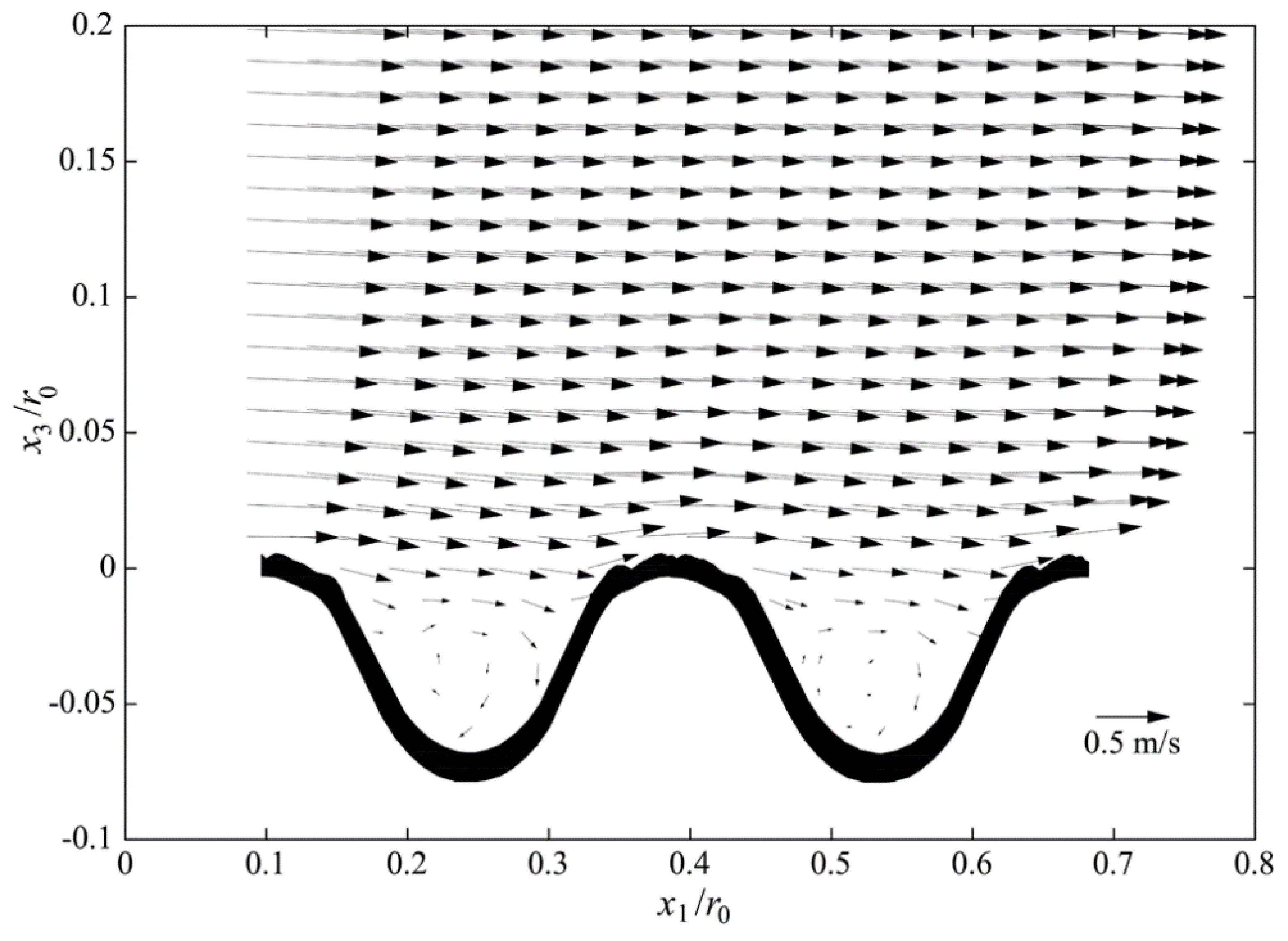
Figure 20.
The experimental stage-discharge curve and the numerical simulations: (a) i = 1.5%; (b) i = 7%.
Figure 20.
The experimental stage-discharge curve and the numerical simulations: (a) i = 1.5%; (b) i = 7%.

Table 1.
The experimental conditions of the local flow velocity tests.
| Test No. | i (%) | Q (L/s) | h (m) | h/D | Re |
|---|---|---|---|---|---|
| 1 | 1.5 | 7.88 | 0.083 | 0.49 (~0.5) | 119,539 |
| 2 | 1.5 | 14.53 | 0.1245 | 0.73 (~0.75) | 165,873 |
| 3 | 7 | 13.63 | 0.0786 | 0.46 (~0.5) | 213,771 |
| 4 | 7 | 25.95 | 0.1185 | 0.69 (~0.75) | 308,736 |
Table 2.
The fluid properties.
| Parameter | Value |
|---|---|
| Air density | 1.225 (g/m3) |
| Water density | 1000 (kg/m3) |
| Air kinematic viscosity | 1.48 × 10⁻⁵ (m2/s) |
| Water kinematic viscosity | 1.0 × 10⁻⁶ (m2/s) |
Table 3.
The grid refinement progression for Test no. 1.
| Parameters | Simulation A | Simulation B | Simulation C (Final) |
|---|---|---|---|
| Ntotal | 0.43 × 10⁶ | 1.02 × 10⁶ | 27.5 × 10⁶ |
| Δx1 (m) | 0.004 | 0.003 | 0.001 |
| Δx2 (m) | 0.004 | 0.003 | 0.001 |
| Δx3 (m) | 0.004 | 0.003 | 0.001 |
Table 4.
The predicted discharge for the tests with velocity profiles.
| Test No. | i (%) | Qmeas. (L/s) | h (cm) | Qcomp. (L/s) | e (%) |
|---|---|---|---|---|---|
| 1 | 1.5 | 7.88 | 8.3 | 7.97 | 1.1 |
| 2 | 1.5 | 14.53 | 12.45 | 14.74 | 1.4 |
| 3 | 7.0 | 13.63 | 7.86 | 15.62 | 14.6 |
| 4 | 7.0 | 25.95 | 11.85 | 29.47 | 13.6 |
Table 5.
The comparison between the numerical and experimental discharge values.
| Test No. | Qexp. (L/s) | Qnum. (L/s) (k-ω) | Deviation (%) | Qnum. (L/s) (k-ω SST) | Deviation (%) |
|---|---|---|---|---|---|
| 1 | 7.88 | 7.84 | −0.51 | 8.00 | 1.52 |
| 2 | 14.53 | 14.25 | −1.93 | 14.73 | 1.38 |
| 3 | 13.63 | 13.20 | −3.15 | 13.91 | 2.05 |
| 4 | 25.95 | 25.50 | −1.73 | 26.01 | 0.23 |
Table 6.
The comparison between the numerical and experimental flow depths.
| Test No. | hexp. (cm) | hnum. (cm) (k-ω) | Deviation (%) | hnum. (cm) (k-ω SST) | Deviation (%) |
|---|---|---|---|---|---|
| 1 | 8.30 | 8.0 | −3.61 | 7.9 | −4.82 |
| 2 | 12.45 | 12.4 | −0.40 | 12.5 | 0.40 |
| 3 | 7.86 | 7.7 | −2.04 | 8.1 | 3.05 |
| 4 | 11.85 | 12.6 | 6.33 | 11.8 | −0.42 |
Table 7.
The comparison between the numerical and experimental flow depths for Tests 5 and 6.
| Test No. | i (%) | Q (L/s) | h (cm) | hnum. (cm) (k-ω) | hnum. (cm) (k-ω SST) |
|---|---|---|---|---|---|
| 5 | 1.5 | 2.42 | 4.5 | 4.3 | 4.4 |
| 6 | 7 | 3.30 | 4.2 | 4.3 | 4.2 |
© 2018 by the authors. Licensee MDPI, Basel, Switzerland. This article is an open access article distributed under the terms and conditions of the Creative Commons Attribution (CC BY) license (http://creativecommons.org/licenses/by/4.0/).
Share and Cite
MDPI and ACS Style
Calomino, F.; Alfonsi, G.; Gaudio, R.; D’Ippolito, A.; Lauria, A.; Tafarojnoruz, A.; Artese, S. Experimental and Numerical Study of Free-Surface Flows in a Corrugated Pipe. Water 2018, 10, 638. https://doi.org/10.3390/w10050638
AMA Style
Calomino F, Alfonsi G, Gaudio R, D’Ippolito A, Lauria A, Tafarojnoruz A, Artese S. Experimental and Numerical Study of Free-Surface Flows in a Corrugated Pipe. Water. 2018; 10(5):638. https://doi.org/10.3390/w10050638
Chicago/Turabian StyleCalomino, Francesco, Giancarlo Alfonsi, Roberto Gaudio, Antonino D’Ippolito, Agostino Lauria, Ali Tafarojnoruz, and Serena Artese. 2018. "Experimental and Numerical Study of Free-Surface Flows in a Corrugated Pipe" Water 10, no. 5: 638. https://doi.org/10.3390/w10050638
Note that from the first issue of 2016, this journal uses article numbers instead of page numbers. See further details here.