Reference Evapotranspiration Variation Analysis and Its Approaches Evaluation of 13 Empirical Models in Sub-Humid and Humid Regions: A Case Study of the Huai River Basin, Eastern China

Abstract

Accurate and reliable estimations of reference evapotranspiration (ET₀) are imperative in irrigation scheduling and water resource planning. This study aims to analyze the spatiotemporal trends of the monthly ET₀ calculated by the Penman–Monteith FAO-56 (PMF-56) model in the Huai River Basin (HRB), eastern China. However, the use of the PMF-56 model is limited by the insufficiency of climatic input parameters in various sites, and the alternative is to employ simple empirical models. In this study, the performances of 13 empirical models were evaluated against the PMF-56 model by using three common statistical approaches: relative root-mean-square error (RRMSE), mean absolute error (MAE), and the Nash–Sutcliffe coefficient (NS). Additionally, a linear regression model was adopted to calibrate and validate the performances of the empirical models during the 1961–2000 and 2001–2014 time periods, respectively. The results showed that the ET_PMF increased initially and then decreased on a monthly timescale. On a daily timescale, the Valiantzas3 (VA3) was the best alternative model for estimating the ET₀, while the Penman (PEN), WMO, Trabert (TRA), and Jensen-Haise (JH) models showed poor results with large errors. Before calibration, the determination coefficients of the temperature-based, radiation-based, and combined models showed the opposite changing trends compared to the mass transfer-based models. After calibration, the performance of each empirical model in each month improved greatly except for the PEN model. If the comprehensive climatic datasets were available, the VA3 would be the recommended model because it had a simple computation procedure and was also very well correlated linearly to the PMF-56 model. Given the data availability, the temperature-based, radiation-based, Valiantzas1 (VA1) and Valiantzas2 (VA2) models were recommended during April–October in the HRB and other similar regions, and also, the mass transfer-based models were applicable in other months.

1. Introduction

Under the background of global warming, reference evapotranspiration (ET₀) has become a crucial agrometeorological variable for meteorological and hydrological process studies, as well as for irrigation scheduling and management, which plays a vital role in the atmosphere, hydrosphere, and biosphere. From the agricultural perspective, its estimation is greatly significant in humid and sub-humid regions like eastern China, where it is vital for determining high crop water requirements and subsequently, for planning and managing irrigation practices [1]. Accurate and reliable estimations of ET₀ are essential for improving water resource planning and management [2,3], farm irrigation demand, and also environmental assessment [4].

Numerous models based on climatic variables have already been employed to calculate the ET₀ in many climatic and hydrogeographic settings [2,5]. For example, the Penman–Monteith FAO-56 (PMF-56) model recommended by the Food and Agricultural Organization (FAO) has been recognized as the most accurate model for estimating the ET₀ over the past few decades [6]. The PMF-56 model has two advantages compared with other models [2,7]. Firstly, it is used globally without any calibrations because of its biophysical basis. Secondly, this model has been well-documented in the existing literature, in which it has been evaluated using a variety of conditions [5]. The main shortcoming of the PMF-56 model is the requirement of large datasets, including the air mean, maximum and minimum temperature, relative humidity, wind speed, and solar radiation. Records of these meteorological input parameters are often with debatable quality or are unavailable for a specific site, especially in some developing countries [1]. In addition, the installation and maintenance of meteorological station instruments can be expensive and complicated [8]. Furthermore, some researchers or institutions may not have access to complete meteorological datasets in some study areas. In the areas where the observed large meteorological data are difficult to obtain, the PMF-56 model is not the best option. To solve this problem, ET₀ estimation models with a fewer errors and a simple computation procedure are preferably applied. Therefore, there is an urgent need to find an accurate, suitable, and simple alternative model to estimate the ET₀ relative to the PMF-56 model when the meteorological datasets are limited or missing.

During recent decades, the empirical models have been developed for estimating the ET₀, which required fewer meteorological parameters or simplified expressions. There are four main climatic models: mass transfer-based, temperature-based, radiation-based, and the combined models. Although a significant number of studies have been performed to evaluate these empirical models in various climatic regions throughout China (e.g., Chen et al. [9]; Cai et al. [7]; Huo et al. [10]; Wen et al. [3]; Liu et al. [11]; and Feng et al. [12]), few such studies have been conducted in humid and sub-humid climatic regions of eastern China [1,13]. Indeed, the performances of the empirical models may vary in various environmental conditions, and local evaluation and calibration are needed [5]. Feng et al. [12] calibrated the Hargreaves model using Bayesian theory in the Sichuan basin of southwestern China. Liu et al. [11] determined the decisive meteorological variables using path analysis to establish the specific models for estimating the ET₀. The above studies mainly adopted temperature-based and radiation-based models to estimate the ET₀; however, the mass transfer-based and combined models have rarely been used in China, and their applicability remains to be tested thoroughly. Hence, it is imperative to carry out research evaluating the performance of the empirical models to determine the best, or a relatively appropriate model for estimating the ET₀ in a humid and sub-humid region.

Due to the simple operability of regression models, practitioners have widely used the simple linear regression model in many studies, as can be found in Mallikarjuna et al. [14], Wen et al. [3], Peng et al. [15], Cobaner et al. [16], Citakoglu et al. [17], and Huo et al. [10]. The regression model expresses the dependence of a response parameter on many independent parameters and is used in modeling a varied range of hydrologic process studies. In addition, Rahimikhoob et al. [4] adopted the regression model to evaluate the performance and characteristics of four empirical models for ET₀ estimation in a subtropical climate in Iran and found that all the performances of the models were improved after the calibration of regional specific coefficients. Similarly, we employ the linear regression model in the present study to assess the performances of 13 empirical models for ET₀ estimation as an alternative approach to the PMF-56.

Owing to the complex relationship between the ET₀ and climatic factors, many practitioners and researchers have adopted computer algorithms to estimate the ET₀ with higher accuracy. Huo et al. [10] trained and tested the artificial neural network (ANN) model for estimating the ET₀ in northwest China and found that the maximum and minimum temperature and relative humidity were the most crucial inputs for this model in arid and semi-arid areas. Tabari et al. [2] evaluated the performance of the support vector machine (SVM), an adaptive neuro-fuzzy inference system (ANFIS), multiple linear regression (MLR), and multiple non-linear regression (MNLR) for ET₀ estimation in a semi-arid highland environment in Iran. They found that the SVM and ANFIS models with inputs of mean temperature, relative humidity, wind speed, and solar radiation showed the best performance. After evaluation of the trained extreme learning machine (ELM), back propagation neural networks optimized by the genetic algorithm (GANN), and wavelet neural networks (WNN), two temperature-based and three radiation-based models were developed in a humid area of southwest China by Feng et al. [18]. Feng et al. [18] recommended the ELM and GANN models as the best alternatives with limited meteorological data. Mehdizadeh et al. [19] tested the performance of the SVM and multivariate adaptive regression splines (MARS) and found that they were better than the empirical models in Iran. Chauhan and Shrivastava [20] investigated the performance of reference evapotranspiration in India using climate-based models and ANNs and found that the ANN models performed better than the climatic-based models in all performance indices. Despite the higher accuracy of the computer algorithms, these algorithms must be implemented through specific software, and the models with particular inputs of climatic factors could not be expressed in straightforward mathematical expressions like the empirical models [16]. Thus, the empirical model as an alternative option to estimate the ET₀ has been recommended in many other studies [20,21,22,23,24].

Except for the aforementioned examples, most of the previous studies have been carried out using a low-precision timescale when there is a need for calibrating the empirical models. Furthermore, Bourletsikas et al. [25] recommended that calibration at a seasonal or even monthly time-step could obtain more accurate daily estimates. To the best of our knowledge, no comprehensive studies have been undertaken to analyze the spatiotemporal trends of monthly ET₀ and evaluate the performances of empirical models in the HRB, eastern China, especially on a monthly timescale, which in itself is the novelty of our research work. Although the performance of 10 empirical models were compared for different sub-regions of mainland China [15], a thorough and detailed study for choosing the best alternative empirical model for the PMF-56 model in the HRB has not been conducted. To fill this research gap, in this study, we chose 13 extensively applied empirical models—including one temperature-based model (Hargreaves–Samani), three mass transfer-based models (Penman, WMO, and Trabert), six radiation-based models (Makkink, Priestly–Taylor, Jensen–Haise, Abtew, Irmak, and Tabari), and three combined models (Valiantzas1, Valiantzas2, and Valiantzas3)—based on their meteorological input parameters and applicability worldwide. Consequently, we propose two hypotheses: (1) the different empirical models will produce significantly different results for the estimation of reference evapotranspiration on a monthly timescale; and (2) the linear regression model can effectively calibrate the 13 empirical models against the PMF-56 model in the HRB. Ultimately, the main objectives of this study are (1) to analyze the spatiotemporal trends of the ET_PMF in the HRB during 1961–2014 on a monthly timescale; (2) to evaluate the performances of 13 empirical models against the PMF-56 model for ET₀ estimation on a daily timescale; (3) to calibrate the 13 empirical models using the daily datasets from 1961–2000 by adopting the linear regression model on a monthly timescale; and (4) to validate the calibrated empirical models by using three statistical approaches during the period of 2001–2014 on a monthly timescale. The outcomes of the study will provide meaningful guidance for agricultural production and hydrological planning and management in this vital region, as well as other regions with the similar climates.

2. Materials and Methods

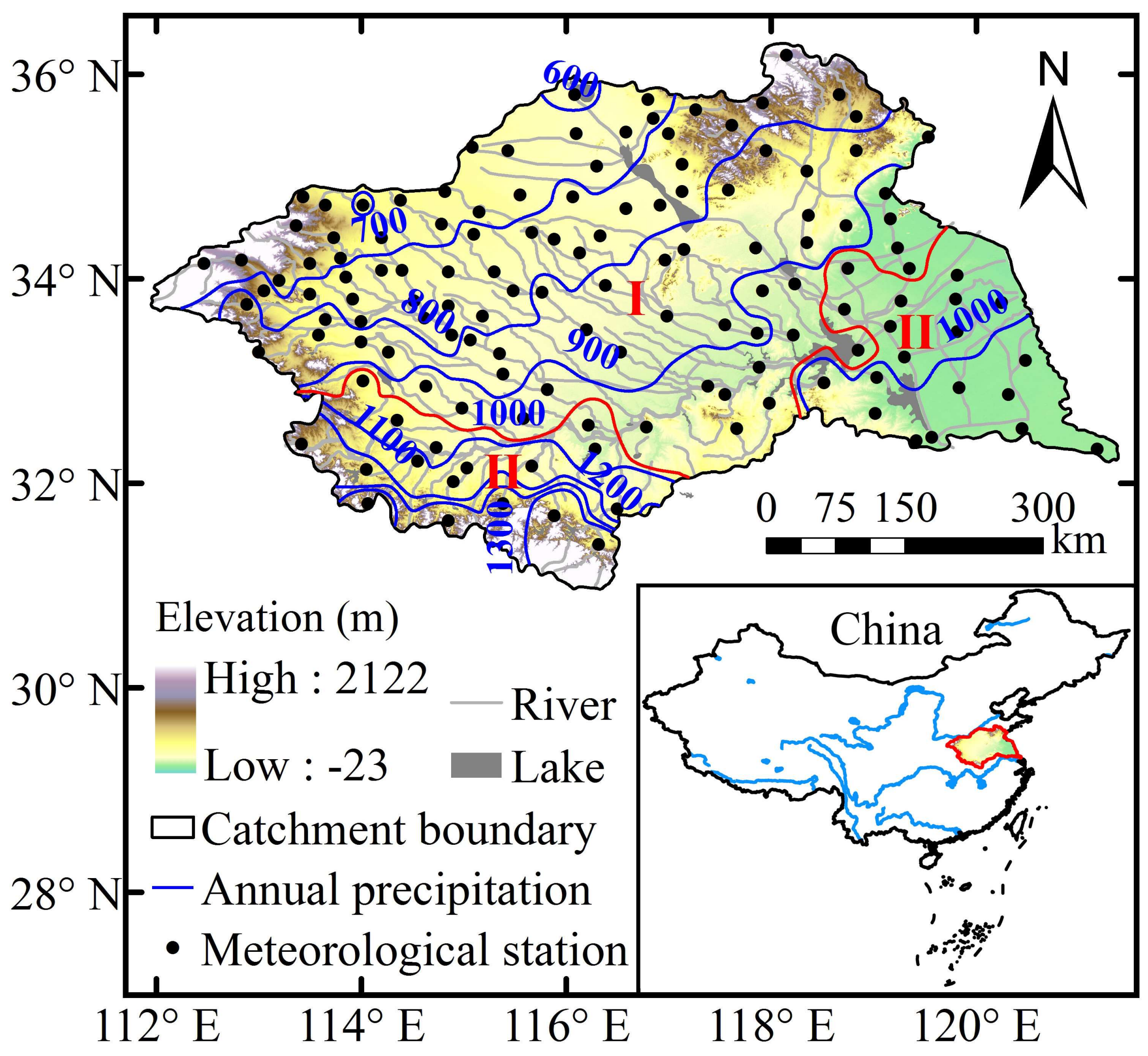
2.1. Study Area and Datasets

The Huai River Basin (HRB) is located in a climate transition zone (111°55′–121°25′ E, 30°55′–36°36′ N) between northern and southern China, with a catchment area of about 270,000 km². The western, southwestern, and northeastern parts of the HRB are mainly mountainous and hilly areas, with the remaining area occupied by broad plains for about two-thirds of the total basin area (Figure 1). The annual average temperature ranges from 11 °C to 16 °C, increasing from north to south, as well as from coast to island areas. The annual mean water surface evaporation ranges from 900 mm to 1500 mm, and relative humidity ranges from 40 to 70%. Annual average precipitation is about 970 mm; more than 50% of rainfall is concentrated in the monsoon season from June to September. With an uneven distribution pattern of precipitation and complex weather systems, the HRB is extremely vulnerable to floods during the rainy season and drought during the dry season.

Daily meteorological data from 137 meteorological stations in the HRB during 1961–2014, including mean temperature (T, °C), maximum temperature (T_max, °C), minimum temperature (T_min, °C), relative humidity (RH, %), wind speed at 2 m height (u₂, m·s⁻¹), sunshine duration (SD, h), and precipitation (P_r, mm), were obtained from the National Meteorological Information Center (NMIC) of the China Meteorological Administration (CMA). Quality control had already been applied to the meteorological datasets by the staff members of the NMIC. Detailed data descriptions can be found at the website http://data.cma.cn/. Specific information for each station is listed in

Table A1. Geospatial information of the meteorological stations in the Huai River Basin.

WMO Number	Stations	Lon. (°E)	Lat. (°N)	H (m)	WMO Number	Stations	Lon. (°E)	Lat. (°N)	H (m)
54836	Yiyuan	118.15	36.18	301.6	58011	Shanxian	116.07	34.80	44.3
54906	Heze	115.43	35.25	50.8	58012	Fengxian	116.58	34.68	40.6
54908	Dongming	115.08	35.28	59.5	58013	Peixian	116.92	34.72	36.7
54910	Liangshan	116.08	35.80	40.8	58015	Dangshan	116.33	34.42	50.9
54913	Ningyang	116.80	35.75	61.2	58016	Xiaoxian	116.97	34.18	39.2
54914	Juye	116.10	35.42	41.1	58017	Xiayi	116.13	34.25	41
54915	Jining	116.58	35.43	45.2	58020	Weishan	117.13	34.85	40.5
54916	Yanzhou	116.85	35.57	53	58024	Zaozhuang	117.58	34.87	74.8
54917	Jinxiang	116.30	35.10	41.3	58026	Pizhou	117.85	34.30	24
54919	Zoucheng	117.00	35.42	78.9	58027	Xuzhou	117.15	34.28	41.9
54920	Sishui	117.27	35.65	110.4	58034	Tancheng	118.37	34.62	38.4
54923	Mengyin	117.92	35.72	202.9	58035	Xinyi	118.35	34.35	29.4
54925	Pingyi	117.62	35.50	167	58036	Donghai	118.73	34.52	35.2
54927	Tengzhou	117.13	35.12	65.9	58038	Shuyang	118.75	34.10	8.8
54929	Feixian	117.95	35.25	120.5	58040	Ganyu	119.12	34.83	9.8
54932	Yishui	118.67	35.80	160.6	58044	Lianyungang	119.17	34.58	4.1
54936	Juxian	118.83	35.58	108.6	58047	Guanyun	119.23	34.30	5
54938	Linyi	118.35	35.05	86.5	58048	Guannan	119.35	34.10	6
54939	Junan	118.83	35.25	113.1	58049	Binhai	119.82	34.03	4.5
54945	Rizhao	119.53	35.38	22.8	58100	Dancheng	115.18	33.63	42.4
57075	Ruzhou	112.83	34.18	214.2	58101	Luyi	115.48	33.88	41.2
57078	Ruyang	112.47	34.15	307.8	58102	Bozhou	115.77	33.87	41.8
57081	Xingyang	113.43	34.80	140.5	58104	Shenqiu	115.07	33.40	42
57083	Zhengzhou	113.65	34.72	111.3	58107	Linquan	115.38	33.07	36.5
57085	Xinmi	113.37	34.52	289.3	58108	Jieshou	115.35	33.27	38.7
57086	Xinzheng	113.73	34.40	111.9	58111	Yongcheng	116.38	33.93	32.7
57087	Changge	113.80	34.20	88.5	58114	Guoyang	116.20	33.50	31.2
57088	Yuzhou	113.50	34.15	117.2	58118	Mengcheng	116.53	33.28	27.5
57089	Xuchang	113.85	34.02	67.7	58122	Suzhou	116.98	33.63	36.7
57090	Zhongmu	114.02	34.72	82.1	58125	Lingbi	117.55	33.55	28.1
57091	Kaifeng	114.38	34.77	73.7	58126	Sixian	117.87	33.47	20.6
57093	Lankao	114.82	34.85	72.2	58129	Wuhe	117.88	33.13	21
57094	Weishi	114.20	34.40	67.5	58130	Suining	117.92	33.88	23.5
57095	Yanling	114.20	34.08	60.4	58131	Suyu	118.23	33.95	28.1
57096	Qixian	114.78	34.53	60.7	58132	Siyang	118.72	33.70	15.6
57098	Fugou	114.40	34.08	59.3	58135	Sihong	118.22	33.45	17
57099	Taikang	114.85	34.07	53.6	58138	Xuyi	118.52	32.98	36.3
57173	Lushan	112.88	33.75	146.9	58139	Hongze	118.85	33.30	19.6
57179	Fangcheng	113.00	33.28	161.5	58140	Lianshui	119.27	33.78	10.2
57180	Jiaxian	113.20	33.98	118.6	58143	Funing	119.80	33.80	3.1
57181	Baofeng	113.05	33.88	137.5	58145	Chuzhou	119.17	33.53	8.3
57182	Xiangcheng	113.50	33.85	81.4	58146	Jianhu	119.82	33.48	3.4
57183	Linying	113.92	33.80	60.8	58147	Jinhu	119.03	33.03	10.9
57184	Yexian	113.65	33.60	86.7	58148	Baoying	119.30	33.23	8.4
57185	Wuyang	113.58	33.45	92.3	58150	Sheyang	120.25	33.77	6.7
57186	Luohe	114.00	33.58	62.1	58158	Dafeng	120.48	33.20	7.3
57188	Xiping	114.00	33.38	60.6	58202	Funan	115.58	32.63	35.7
57192	Huaiyang	114.85	33.73	46.3	58203	Fuyang	115.82	32.92	38.6
57193	Xihua	114.52	33.78	53.5	58207	Huangchuan	115.03	32.15	42.9
57194	Shangcai	114.27	33.28	60.8	58208	Gushi	115.67	32.17	57.9
57195	Chuanhuiqu	114.62	33.62	47.6	58210	Yingshang	116.22	32.57	25.5
57196	Xiangcheng	114.88	33.45	44.4	58214	Huoqiu	116.28	32.33	36.9
57285	Tongbai	113.42	32.38	149.1	58215	Shouxian	116.78	32.55	23.5
57290	Zhumadian	114.02	33.00	83.3	58221	Bengbu	117.38	32.95	26
57292	Pingyu	114.63	32.95	44	58222	Fengyang	117.55	32.87	28
57293	Xincai	114.98	32.73	39.1	58223	Mingguang	117.98	32.78	35.6
57295	Zhengyang	114.35	32.62	79.7	58225	Dingyuan	117.67	32.53	76.7
57296	Xixian	114.73	32.35	50.1	58240	Tianchang	119.02	32.68	21
57297	Xinyang	114.05	32.13	115.1	58243	Xinghua	119.83	32.93	7.3
57298	Luoshan	114.55	32.22	56.1	58244	Jiangdu	119.57	32.45	10.3
57299	Guangshan	114.90	32.02	50.6	58245	Yangzhou	119.42	32.42	9.9
57390	Jigongshan	114.07	31.80	733.5	58251	Dongtai	120.32	32.87	5.1
57396	Xinxian	114.85	31.63	130.8	58254	Haian	120.45	32.53	5.2
58001	Suixian	115.10	34.43	57.1	58264	Rudong	121.18	32.33	3.4
58002	Caoxian	115.55	34.82	50	58301	Shangcheng	115.38	31.80	79.1
58004	Minquan	115.15	34.65	61	58306	Jinzhai	115.88	31.68	94
58005	Shangqiu	115.67	34.45	51	58311	Luan	116.50	31.75	60.4
58006	Yucheng	115.88	34.38	47.2

Note: The data period for each station is from 1961 to 2014.

. All stations were divided into two climate zones, namely humid and sub-humid regions. The subdivision of these two climate zones is mainly according to the global aridity index (AI) adopted by the United Nations Convention to Combat Desertification [26,27,28]. The AI is defined as the ratio of annual average precipitation to reference evapotranspiration, and the classification standards of humid and sub-humid regions are as follows: AI > 1 for humid regions and 0.5 < AI < 1 for sub-humid regions. The demarcation line between humid and sub-humid regions is displayed in Figure 1. The description of the main climatic factors in each region of the HRB during the study period is presented in

Table 1. Annual means of the main climatic factors in the sub-humid and humid regions and the whole HRB during 1961–2014.

Region	T (°C)	Tmax (°C)	Tmin (°C)	RH (%)	u2 (m·s−1)	Rs (MJ·m−2·d—1)	Pr (mm·a—1)	ET0 (mm·a—1)
Sub-humid (I)	14.45	19.93	9.84	70.29	1.86	15.08	783.05	981.23
Humid (II)	15.03	19.88	11.12	75.96	1.95	14.85	1049.63	936.89
Whole	14.60	19.92	10.18	71.78	1.88	15.02	853.10	969.57

Note: R_s is the solar radiation (MJ·m⁻²·d⁻¹).

.

2.2. Penman–Monteith FAO-56 Model (PMF-56 Model)

Due to the absence of the observation of lysimeters, the Penman–Monteith FAO-56 model (PMF-56), which was proposed by Allen et al. [6], was adopted as standard all over the world and is considered the best model for estimating reference evapotranspiration [1,29,30,31]. The exact expression is shown in the following Equation (1):

$$E{T}_{PMF}=\frac{0.408\Delta \left(R_n-G\right)+\gamma \frac{900}{T+273}{u}_2\left(e_s-e_a\right)}{\Delta +\gamma \left(1+0.34u_2\right)}$$

(1)

where ET_PMF is the daily reference evapotranspiration (mm·d⁻¹), ∆ is the slope of the vapor pressure curve (kPa·°C⁻¹), R_n is the net solar radiation (MJ·m⁻²·d⁻¹), G is the soil heat flux density (MJ·m⁻²·d⁻¹), γ is the psychrometric constant (kPa·°C⁻¹), T is the daily mean air temperature at 2 m height (°C), u₂ is the wind speed at 2 m height (m·s⁻¹), e_s is the saturation vapor pressure (kPa), and e_a is the actual vapor pressure (kPa). The detailed calculations of the parameters in Equation (1) can be found in the literature [1,6].

2.3. Empirical Models

Our preliminary evaluation of the 13 empirical models was based on the acceptance of their meteorological input parameters and the applicability of the models worldwide. These 13 empirical ET₀ models, which commonly performed well in various regions of the world [24,32,33,34,35,36,37,38,39,40], were selected to compare to the PMF-56 model. The combined models included the three Valiantzas equations [41,42], which were proposed to simplify the PMF-56 equation. The three Valiantzas [41,42] equations were comparatively new, and their performances had not been validated in eastern China. The Hargreaves–Samani equation (HS) was adopted in the present study because the PMF-56 manual recommended the use of the HS as a less complex model mainly requiring data on temperature and extraterrestrial radiation. Thus, the 13 empirical models employed in this study can be divided into the following four categories: one temperature-based model (Hargreaves–Samani), three mass transfer-based models (Penman, WMO, and Trabert), six radiation-based models (Makkink, Priestly–Taylor, Jensen–Haise, Abtew, Irmak, and Tabari), and three combined models (Valiantzas1, Valiantzas2, Valiantzas3). The specific calculation equations, main input variables, and references are presented in

Table 2. Original forms of the 13 empirical models.

NO.	Models	Models Input	Equations	References
	Temperature-based
1	Hargreaves–Samani	T, Tmax, Tmin	$E{T}_{HS}=0.0023·0.408R_a\left(T+17.8\right){\left(T_{max}-T_{min}\right)}^{0.5}$	[32]
	Mass transfer-based
2	Penman	u2, es − ea	$E{T}_{PEN}=0.35\left(1+0.98/100u_2\right)\left(e_s-e_a\right)$	[33]
3	WMO	u2, es − ea	$E{T}_{WMO}=\left(0.1298+0.0934u_2\right)\left(e_s-e_a\right)$	[34]
4	Trabert	u2, es − ea	$E{T}_{TRA}=3.075u_2{}^{0.5}\left(e_s-e_a\right)$	[35]
	Radiation-based
5	Makkink	Rs, T	$E{T}_{MAK}=0.61\frac{\Delta }{\Delta +\gamma }\frac{R_s}{\lambda }-0.12$	[36]
6	Priestley–Taylor	Rn, T	$E{T}_{PT}=1.26\frac{\Delta }{\Delta +\gamma }\frac{R_n-G}{\lambda }$	[37]
7	Jensen–Haise	Rs, T	$E{T}_{JH}=\left(0.025T+0.08\right)\frac{R_s}{\lambda }$	[38]
8	Abtew	Rs, Tmax	$E{T}_{ABT}=\frac{1}{56}\frac{R_s{T}_{max}}{\lambda }$	[39]
9	Irmak	Rs, T	$E{T}_{IRM}=0.149R_s+0.079T-0.611$	[40]
10	Tabari	Rs, Tmax, Tmin	$E{T}_{TAB}=0.156R_s-0.0112T_{max}+0.0733T_{min}-0.478$	[24]
	Combined
11	Valiantzas1	Rs, T, RH	$E{T}_{VA1}=0.0393R_s\sqrt{T+9.5}-0.19R_s{}^{0.6}{\varphi }^{0.15}+0.078\left(T+20\right)\left(1-\frac{RH}{100}\right)$	[41,42]
12	Valiantzas2	Rs, T, Tmin	$E{T}_{VA2}=0.0393R_s\sqrt{T+9.5}-0.19R_s{}^{0.6}{\varphi }^{0.15}+0.0061\left(T+20\right){\left(1.12T-T_{min}-2\right)}^{0.7}$	[41,42]
13	Valiantzas3	Rs, T, RH, u2	$E{T}_{VA3}=0.0393R_s\sqrt{T+9.5}-0.19R_s{}^{0.6}{\varphi }^{0.15}+0.048\left(T+20\right)\left(1-\frac{RH}{100}\right)u_2{}^{0.7}$	[41,42]

Note: R_a is the extraterrestrial radiation (MJ·m⁻²·d⁻¹), R_s is the solar radiation (MJ·m⁻²·d⁻¹), R_n is the net solar radiation (MJ·m⁻²·d⁻¹), T, T_max, and T_min are mean, maximum, and minimum temperature (°C), respectively, u₂ is the wind speed at 2 m height (The unit of u₂ is in m·s⁻¹ in all equations except the Penman model, where u₂ is in miles·d⁻¹), e_s and e_a are saturation and actual vapor pressure, respectively (The units of e_s and e_a are in hPa in all equations except the Penman model, where e_s and e_a are in mmHg.), RH is the relative humidity (%), ∆ is the slope of the vapor pressure curve (kPa·°C⁻¹), γ is the psychrometric constant (kPa·°C⁻¹), λ is the latent heat of vaporization (≈2.45 MJ·kg⁻¹), G is the soil heat flux density (MJ·m⁻²·d⁻¹), and φ is the latitude (rad). The abbreviations of the 13 empirical models are arranged in order that the models appear in Table 2: HS, PEN, WMO, TRA, MAK, PT, JH, ABT, IRM, TAB, VA1, VA2, and VA3.

.

2.4. Performance Evaluation Approaches

In this study, the performance of the 13 empirical models was evaluated by adopting three statistical approaches: relative root-mean-square error (RRMSE), mean absolute error (MAE) and the Nash–Sutcliffe coefficient (NS) [12,43]. The following Equations (2)–(4) are used to evaluate the performances of the 13 empirical models:

$$RRMSE=\frac{RMSE}{E{T}_{PMF,mean}}=\frac{\sqrt{\frac{1}{n}{{\displaystyle \sum }}_{i=1}^n{\left(E{T}_{EMP}^i-E{T}_{PMF}^i\right)}^2}}{E{T}_{PMF,mean}}$$

(2)

$$MAE=\frac{{{\displaystyle \sum }}_{i=1}^n\left|E{T}_{EMP}^i-E{T}_{PMF}^i\right|}{n}$$

(3)

$$NS=1-\frac{{{\displaystyle \sum }}_{i=1}^n{\left(E{T}_{EMP}^i-E{T}_{PMF}^i\right)}^2}{{{\displaystyle \sum }}_{i=1}^n{\left(E{T}_{PMF}^i-E{T}_{PMF,mean}\right)}^2}$$

(4)

where $E{T}_{PMF}^i$ and $E{T}_{EMP}^i$ are daily reference evapotranspiration estimated by the PMF-56 model and the 13 empirical models, respectively, $n$ is number of the sample size, and $E{T}_{PMF,mean}$ is the mean value of $E{T}_{PMF}$. The $\mathrm{RRMSE}$ is dimensionless, with the value ranging from 0 to $\infty$. The $\mathrm{MAE}$ is in mm·d⁻¹. The closer the value of the $\mathrm{RRMSE}$ or the $\mathrm{MAE}$ to 0, the better the performance of empirical equations. The $\mathrm{NS}$ is dimensionless, with the value ranging from 1 to $-\infty$, the closer the value of the $\mathrm{NS}$ to 1, the better the performance of empirical models.

2.5. Calibration and Validation of the Empirical Models

As recommended by Allen et al. [6], the linear regression model was employed to calibrate and validate the empirical models against the PMF-56 model. The specific expression is shown in the below Equation (5):

$$E{T}_{PMF}=a·E{T}_{EMP} + b$$

(5)

where $E{T}_{PMF}$ and $E{T}_{EMP}$ represent the daily reference evapotranspiration estimated by the PMF-56 model and the 13 empirical models, respectively, and $a$ and $b$ are calibrated empirical coefficients.

2.6. Trend Test

The nonparametric Mann–Kendall (MK) test [44,45] was applied to identify the trend of the ET₀. The MK test statistic (Z) follows the standard normal distribution with a mean of 0 and variance of 1 under the null hypothesis of no trend in the ET₀. The null hypothesis is rejected if |Z| ≥  Z_1−β/2 at a significance level of β, where Z_1−β/2 is the (1 − β/2)–quantile. If the Z value is positive (or negative), then the ET₀ has an increasing (or decreasing) trend. As β  =  0.05, if |Z|  > 1.96, the trend is significant. In addition, Theil–Sen’s slope estimator (β) [46,47] is used to determine the extent of a trend. This method has been usually used to detect the slope of a trend in a hydrometeorological time series dataset, which can be found in the literature [1,13,48]. The spatial distributions of the monthly ET₀ and its trends are mapped by the inverse distance weighted (IDW) interpolation model in ArcGIS (version 9.3) software.

3. Results and Discussion

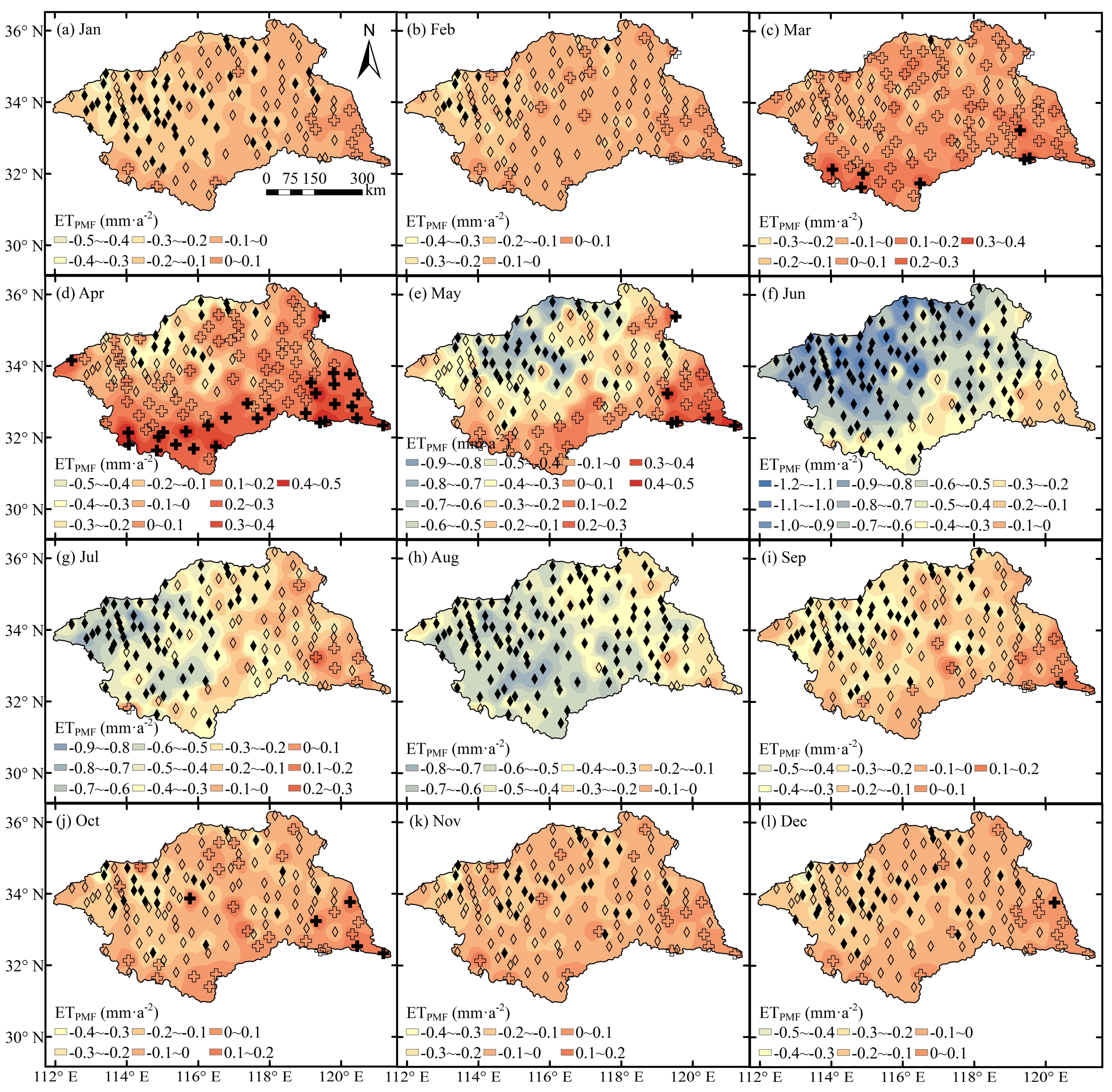
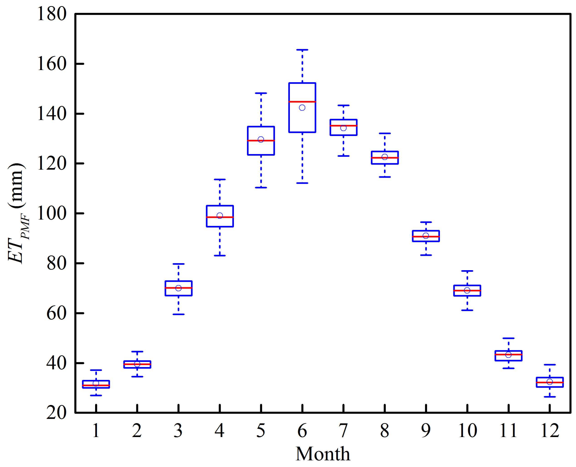
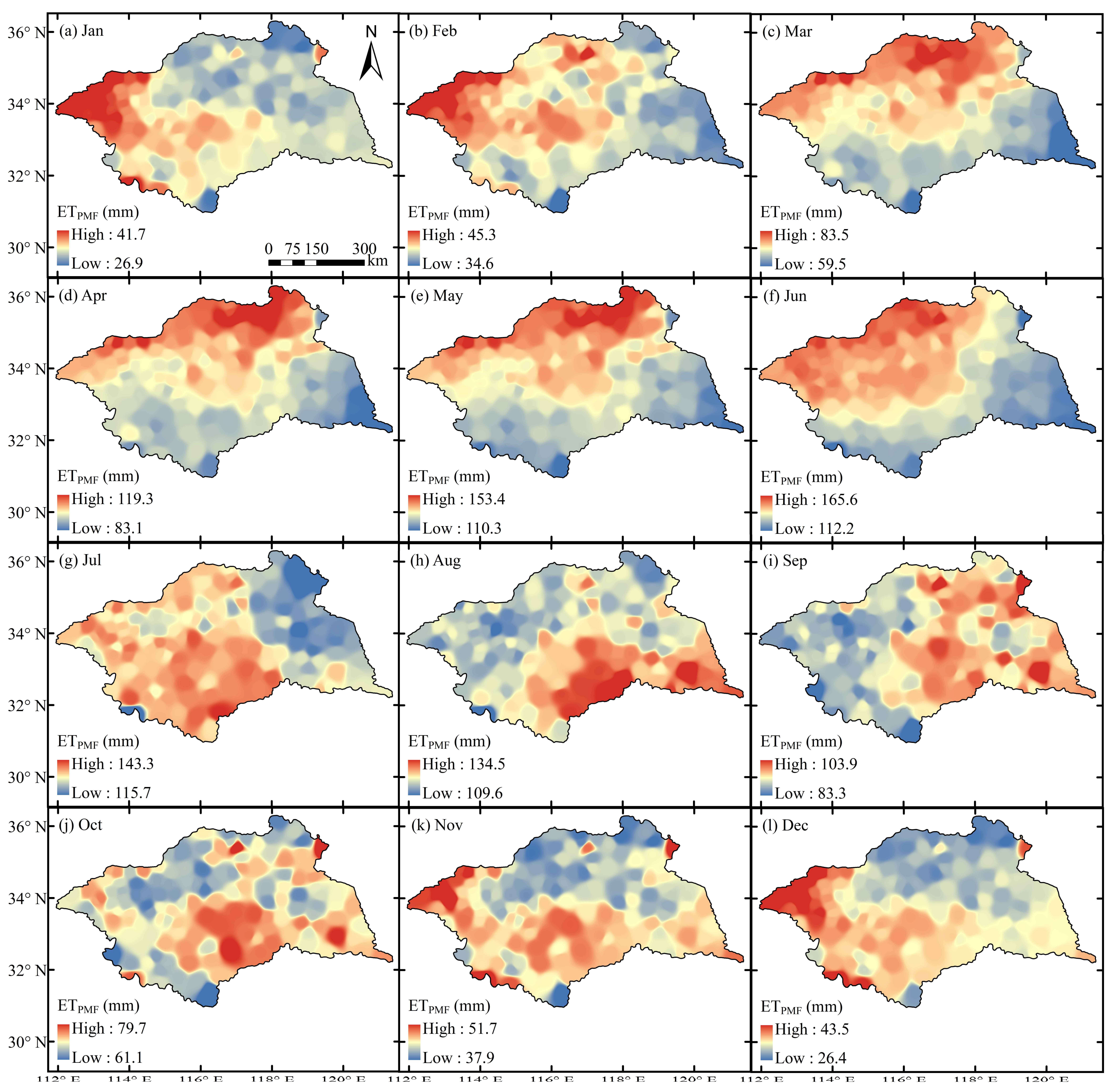
3.1. Monthly Variations of the ET_PMF

As shown in Figure 2, the ET_PMF increased initially and then decreased on a monthly timescale, with the highest value appearing in June and the lowest value in January. Meanwhile, the ET_PMF also revealed large regional differences in April, May, and June, which were especially obvious in June, with the value ranging from 112 mm to 165 mm. Similar monthly trends of the ET_PMF could also be detected in other regions of China, such as the Yellow River Basin [49], northwest China [50], and the Sanjiang Plain in northeast China [51]. The spatial distribution of the ET_PMF results showed a similar tendency of temporal distribution in the HRB (Figure 3). From January to June, the highest-value region of the ET_PMF shifted from the northwest to the northern parts of the HRB, generally demonstrating a gradually increasing trend from south to north. However, from July to December, the highest ET_PMF existed in the central and western parts of the HRB, then shifted to the southeastern parts in August, September, and October, and then shifted back to the southern and northwestern parts in November and December. Different distribution patterns of the ET_PMF were found on a seasonal timescale in the HRB [13]. The ET_PMF represented an obvious spatial evolution pattern on a monthly timescale.

In this study, for a comprehensive understanding of the ET_PMF trends on a monthly timescale in the HRB, the MK test and Sen’s slope estimator were employed. As shown in

Table 3. Temporal trends of the ET_PMF (mm·a⁻²) on a monthly timescale during 1961–2014 in the HRB.

Parameters	Jan	Feby	Mar	Apr	May	Jun	Jul	Aug	Sep	Oct	Nov	Dec
β	−0.108 *	−0.075	0.022	0.030	−0.252	−0.628 ***	−0.330 **	−0.460 ***	−0.155	−0.081	−0.082	−0.089
Z	−2.074	−1.015	0.149	0.269	−1.701	−4.148	−2.716	−4.252	−1.925	−0.985	−1.343	−1.641

Note: *, **, and *** denote the significance levels of 0.05, 0.01, and 0.001, respectively. β is the estimated slope trend of the ET_PMF, and β > 0 and β < 0 signify an upward and a downward trend, respectively. Z is the Mann–Kendall test statistic. Note: Jan, Feb, Mar, Apr, May, Jun, Jul, Aug, Sep, Oct, Nov, and Dec are the abbreviations of January, February, March, May, June, July, August, September, October, November, and December, respectively.

and Figure 4, on a temporal scale, the ET_PMF exhibited significant decreasing trends in January, June, July, and August, with the values of −0.108 mm·a⁻², −0.628 mm·a⁻², −0.330 mm·a⁻², and −0.460 mm·a⁻², respectively. However, in March and April, the ET_PMF demonstrated slightly non-significant increasing trends. Similar to the results in Figure 2, the magnitude of the ET_PMF trends on a spatial scale were higher in June. Particularly, in January, the ET_PMF showed significant decreasing trends in the central and northwestern parts of the HRB, while a non-significant increasing trend of the ET_PMF was detected in some parts of the southwest and southeast of the HRB. Similar trends were identified in September, November, and December, while the magnitude of the ET_PMF trends was much smaller than that in January. In February and October, the stations with significant decreasing ET_PMF trends mainly existed in the northwest of the HRB, and the stations with increasing ET_PMF trends were found in the northeast and southeast of the HRB. In March, about 56% of stations exhibited increasing ET_PMF trends, with a few stations showing significant increasing trends distributed in the southwest and southeast of the HRB. In April, about 62% of stations showed increasing ET_PMF trends, with about 34% of stations distributed in the southern parts of the HRB accounting for the significant increasing trends. Meanwhile, only about 12% of stations located in the north of the HRB exhibited significant decreasing trends in the ET_PMF. However, in May, the proportion of stations with significant decreasing ET_PMF trends in the northern part of the HRB increased to 33%, while the proportion of stations with significant increasing ET_PMF trends decreased to 4% of all stations that were mainly distributed in the southeast of the HRB. Unlike in other months, the ET_PMF showed significant decreasing trends in almost the whole HRB in June and August, accounting for about 89% and 91% of stations, respectively, except for a few stations that exhibited non-significant decreasing trends in the southeast region. Nevertheless, significant decreasing trends of the ET_PMF in July were mainly distributed in the northwestern part of the HRB, with about 54% of stations occupied.

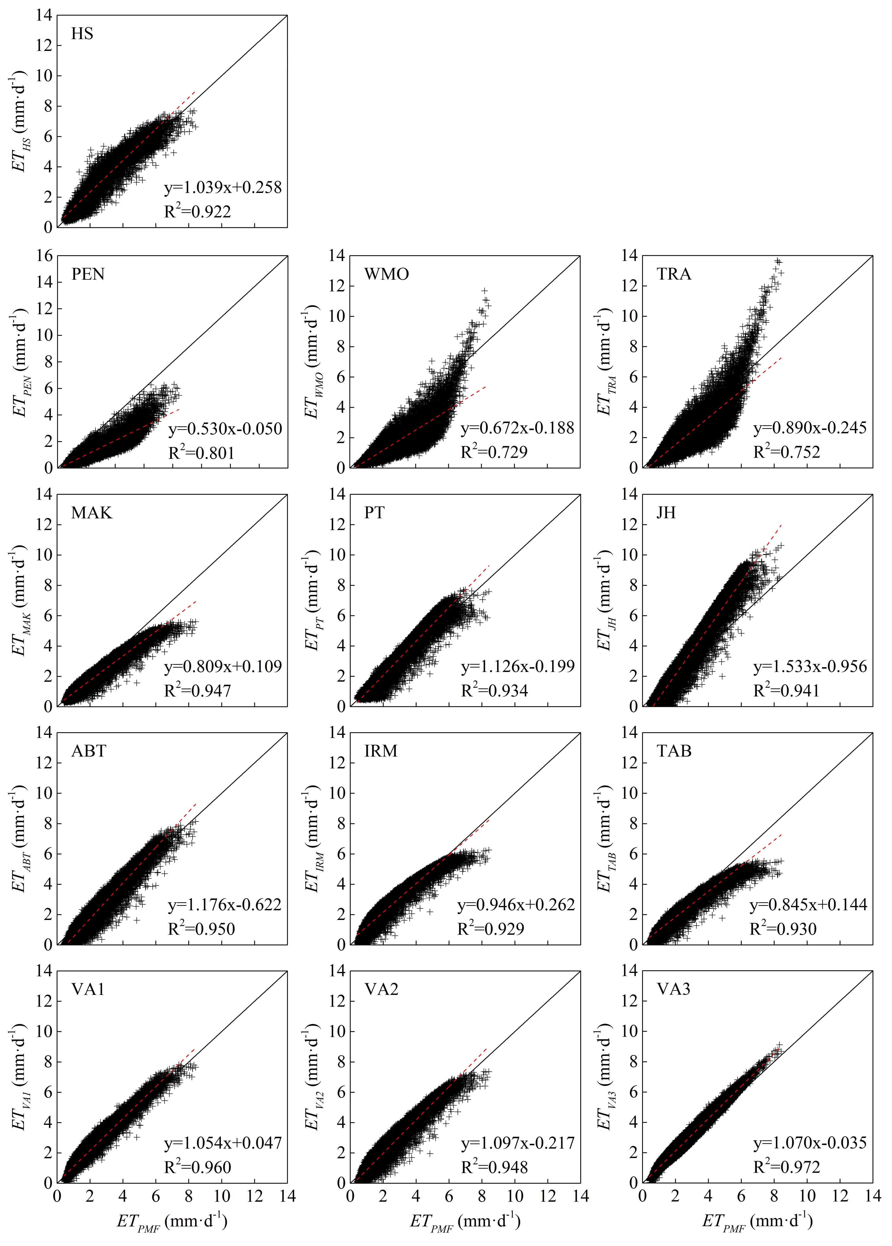
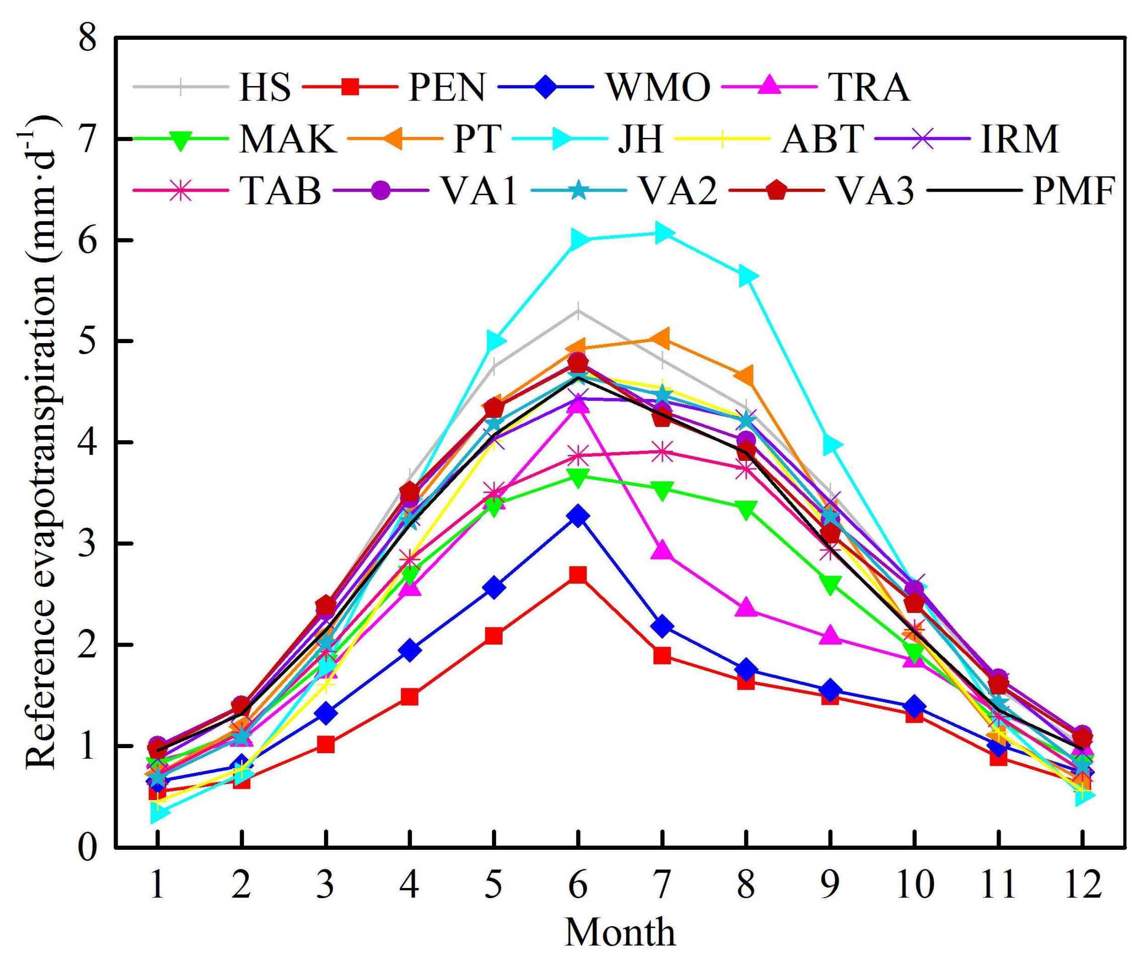
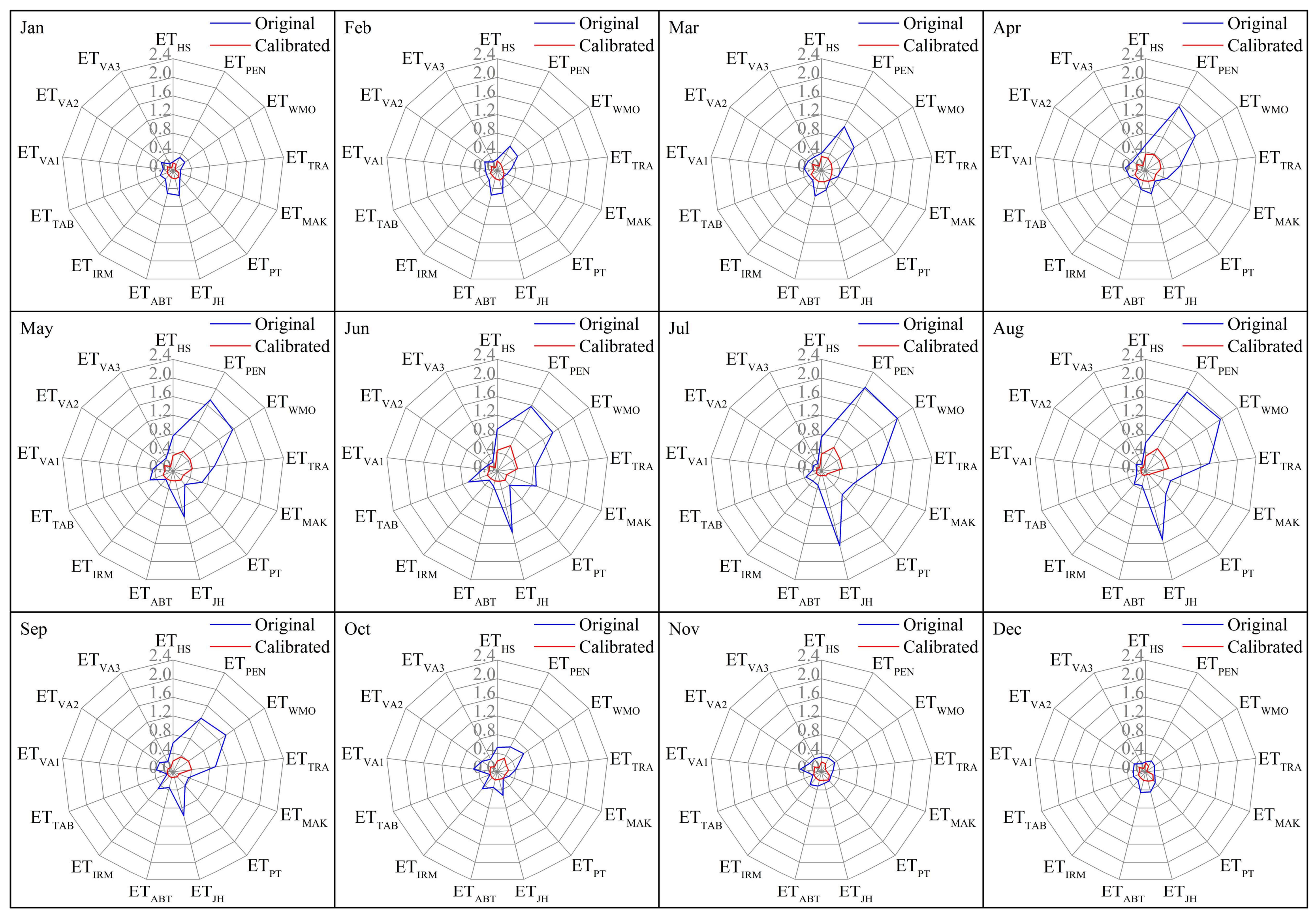
3.2. Performance Evaluation of the 13 Empirical Models in the HRB

Figure 5 shows the scatter plots of reference evapotranspiration estimated by the PMF-56 model (ET_PMF) and the 13 empirical models (ET_EMP) in the HRB. As seen in Figure 5, climatic-based models, such as the temperature-based model (HS), radiation-based models (MAK, PT, JH, ABT, IRM, and TAB), and the combined models (VA1, VA2, and VA3) performed better than the mass transfer-based models (PEN, WMO, and TRA), with all the scatters of the ET_EMP distributed along the 1:1 line and the R-squared greater than 0.9. Among the well-performing models, the HS, PT, JH, ABT, VA1, VA2, and VA3 models overestimated the ET₀ in the whole HRB, with the slope of the linear fit line greater than 1, and the MAK, IRM, and TAB models underestimated the ET₀, with the slope of the linear fit line less than 1. However, the performance of the mass transfer-based models was not satisfactory, with the values of the determination coefficients at less than 0.801. Furthermore, the scatters of the mass transfer-based models are more dispersed, generally underestimating the ET₀ with large errors.

For better evaluation of each empirical model, the statistical analysis, including the RRMSE, the MAE, and the NS, are shown in

Table 4. Statistical analysis of the 13 empirical models versus the PMF-56 model for estimating daily reference evapotranspiration in the HRB from 1961 to 2014.

Parameters	ETHS	ETPEN	ETWMO	ETTRA	ETMAK	ETPT	ETJH	ETABT	ETIRM	ETTAB	ETVA1	ETVA2	ETVA3
RRMSE	0.222	0.580	0.500	0.364	0.217	0.195	0.417	0.195	0.161	0.190	0.147	0.160	0.126
MAE	0.475	1.301	1.079	0.723	0.440	0.411	0.870	0.427	0.347	0.350	0.309	0.340	0.267
NS	0.853	−0.006	0.250	0.604	0.859	0.886	0.479	0.886	0.923	0.892	0.935	0.924	0.953

. In the temperature-based model, the HS model showed average performance, with the values of the RRMSE, the MAE, and the NS were 0.222, 0.475, and 0.853, respectively. The simulation accuracy is higher than that in the Sichuan Basin of southwestern China [12] (where the cloud cover is relatively large, and the solar radiation is reduced, ultimately influencing the estimation results of the ET₀) and also different sub-regions of mainland China [15]. Of the mass transfer-based models, the performance of each model followed the sequence of TRA > WMO > PEN. Considering the results of large errors shown in Figure 5 and values of the RRMSE, the MAE, and the NS, these three models cannot be used as appropriate alternatives, especially the PEN model (for which the values of the RRMSE, the MAE, and the NS were 0.580, 1.301, and −0.006, respectively). Of the radiation-based models, all the models performed well except the JH, for which the values of the RRMSE, the MAE, and the NS were 0.417, 0.870, and 0.419, respectively. The overall performances followed the order of IRM > TAB > PT > ABT > MAK > JH. The poor performance of JH agreed with the results of Ahooghalandari et al. [52] in Australia. In the combined models, all the statistical parameters of each model performed better in estimating the ET₀ than the others, especially the VA3 model, for which the values of the RRMSE, the MAE, and the NS were 0.126, 0.267, and 0.953, respectively, followed closely by VA1 and VA2. Based on the aforementioned discussion, on a daily timescale, the VA3 model is the best alternative model to the PMF-56 model for estimating the ET₀ in the HRB.

In earlier studies, Mehdizadeh et al. [19] reported that the mass transfer-based models showed the worst performance, while the combined models exhibited the best accuracy. The higher precision of the combined models might be due to the combination of the most suitable and important meteorological parameters incorporated therein (e.g., T from the temperature-based model, u₂ and RH from the mass transfer-based models, and R_s from the radiation-based models). Tabari et al. [24] also tested 10 mass transfer-based models in the humid conditions of Iran and found that some of their performances were poor and had underestimated the results. Our results are in good agreement with the findings of Tabari et al. [24]. In this study, the VA3 model showed the best accuracy because of the combination of the T, RH, u₂, and R_s parameters, which play a vital role in ET₀ estimation. Similar findings were also found in Tanzania and southwestern Kenya in eastern Africa [53], India [20], and western Australia [54]. In addition, the better performance of the radiation-based models was mainly due to the important role of the R_s parameter in ET₀ estimation in humid climates [55].

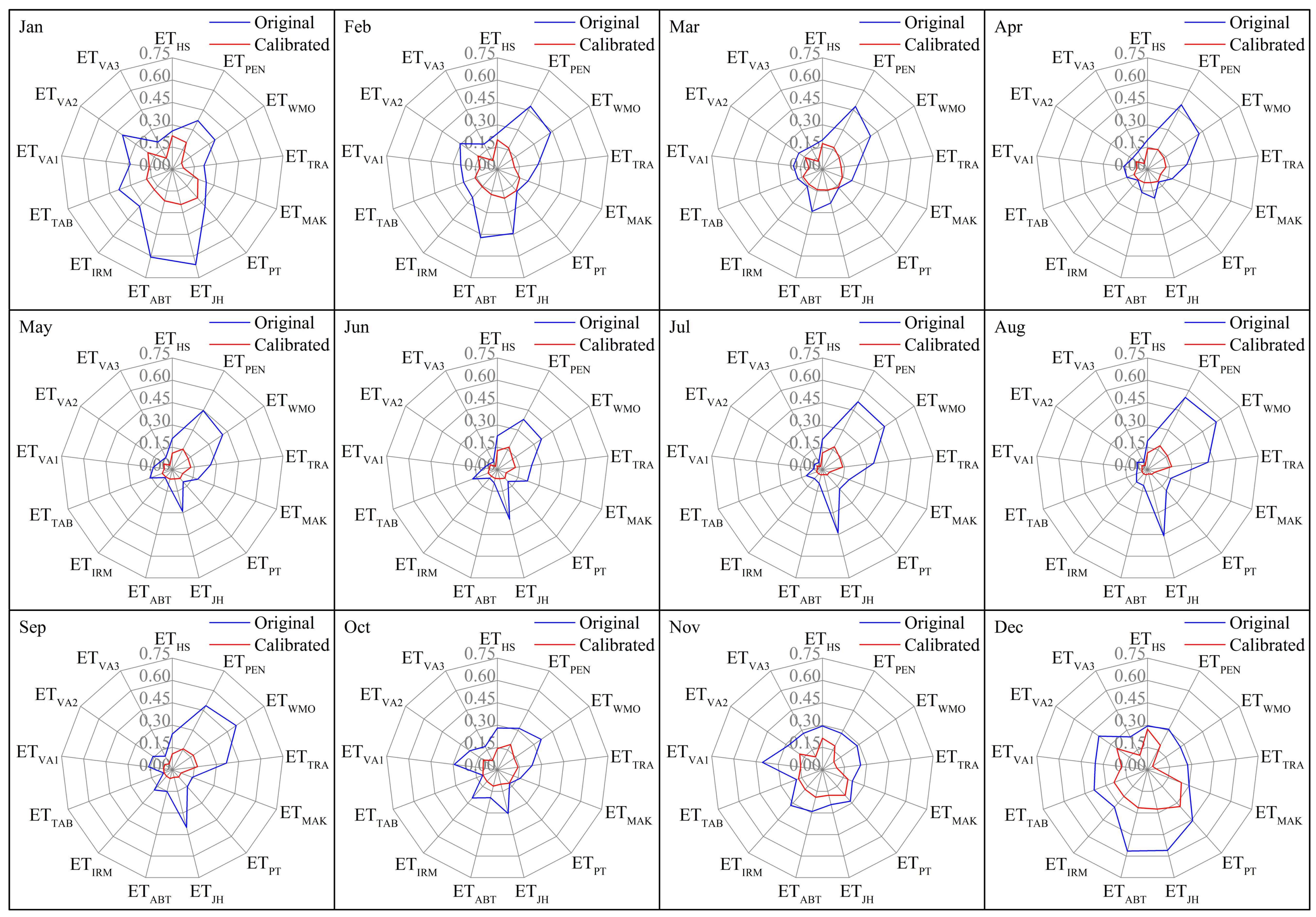
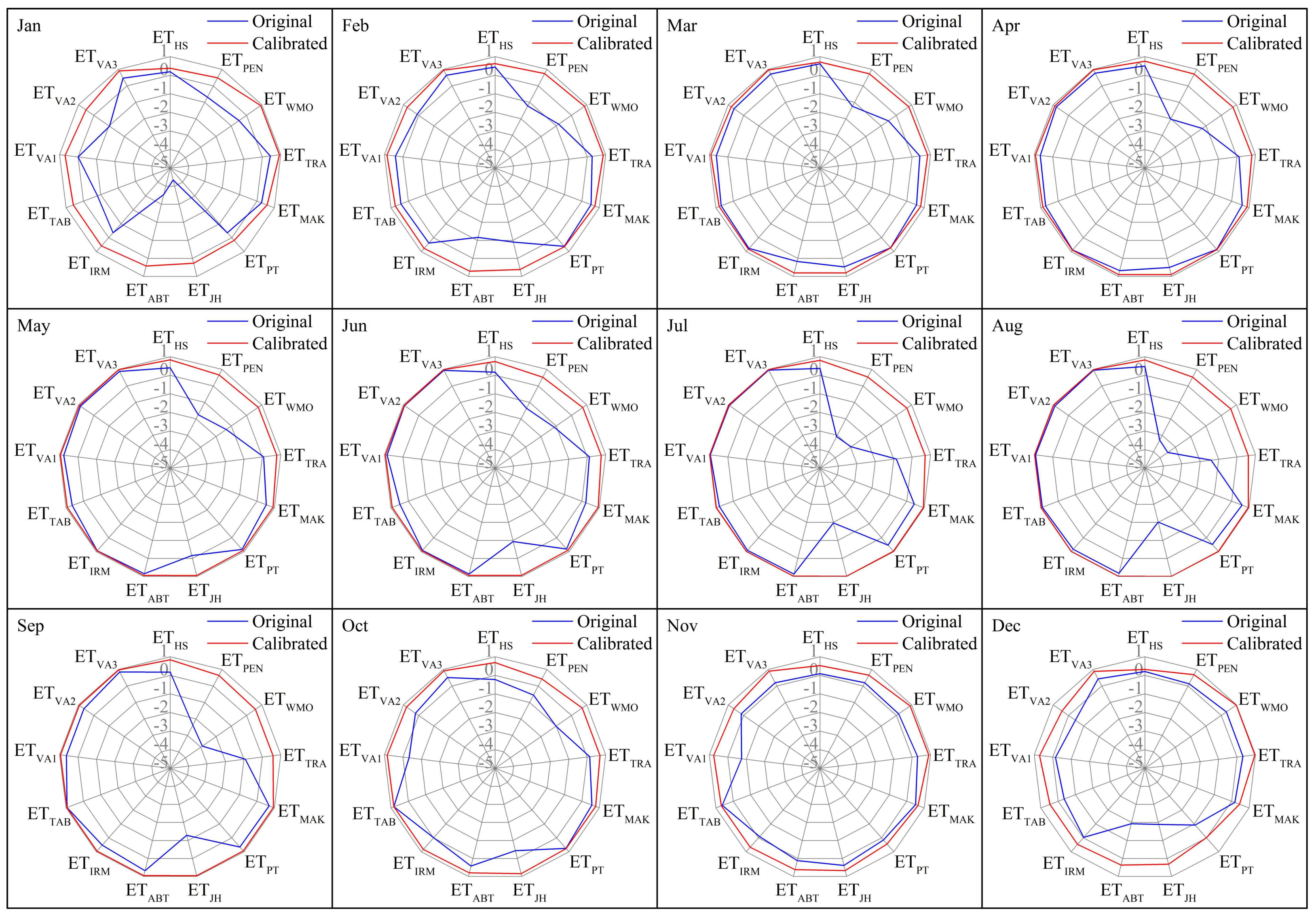
3.3. Calibration of the Empirical Models

As seen in Figure 5 and Table 4, it has been found that each empirical model has more or less errors when estimating reference evapotranspiration compared with that estimated by the PMF-56 model to some extent. In Figure 6, the monthly ET_EMP calculated by the 13 empirical models were compared with the ET_PMF on a monthly timescale. Evidently, the mass transfer-based models (PEN, WMO, and TRA) have different monthly change trends compared to other models, which might be responsible for their poor performance. The underestimation of these three mass transfer-based models was in accordance with the results of Tabari et al. [24] in Iran, although with similar humid conditions, some differences also existed in the monthly average trend. Except for the mass transfer-based models, despite the analogous monthly change trends between the other empirical models and the PMF-56 model, there was still some obvious overestimation (JH, HS, and PT) and underestimation (TAB and MAK) on the monthly timescale. Taking JH model as an example, it overestimated the ET₀ greatly from April to October, while underestimating the ET₀ in other months. Jensen et al. [56], Tabari et al. [24], and Tegos et al. [57] also reported that the JH model tends to overestimate the ET₀ in humid climate conditions. This difference can also be confirmed in Table 4.

Due to the large differences estimated by the empirical models on a monthly timescale, we decided to calibrate the empirical models from month to month. In this study, the 13 empirical models were calibrated using the meteorological datasets from 1961 to 2000 by establishing the linear regression model between the ET_PMF and the ET_EMP. The specific calibration coefficients can be found in

Table 5. The calibration coefficients between the ET_PMF and ET_EMP in monthly timescale during 1961–2000.

Month	Parameters	ETHS	ETPEN	ETWMO	ETTRA	ETMAK	ETPT	ETJH	ETABT	ETIRM	ETTAB	ETVA1	ETVA2	ETVA3
January	a	0.671	1.188	0.783	0.639	0.709	0.868	0.477	0.562	0.467	0.562	0.606	0.506	0.613
	b	0.316	0.329	0.443	0.410	0.376	0.334	0.804	0.727	0.578	0.588	0.370	0.627	0.364
	R2	0.350	0.814	0.943	0.958	0.428	0.114	0.207	0.354	0.430	0.394	0.703	0.402	0.899
February	a	0.825	1.311	0.851	0.685	0.908	1.244	0.712	0.721	0.648	0.772	0.680	0.665	0.664
	b	0.181	0.478	0.626	0.589	0.274	−0.149	0.834	0.797	0.466	0.455	0.381	0.614	0.394
	R2	0.658	0.871	0.891	0.913	0.665	0.570	0.578	0.661	0.677	0.620	0.861	0.696	0.954
March	a	0.902	1.443	0.826	0.687	0.995	1.098	0.763	0.785	0.830	0.983	0.761	0.748	0.721
	b	0.000	0.747	1.034	0.953	0.301	−0.175	0.786	0.878	0.270	0.234	0.380	0.621	0.409
	R2	0.743	0.880	0.834	0.868	0.779	0.723	0.779	0.795	0.783	0.754	0.911	0.796	0.975
April	a	0.946	1.338	0.763	0.636	1.014	0.964	0.663	0.756	0.987	1.144	0.792	0.770	0.770
	b	−0.269	1.276	1.677	1.556	0.435	−0.035	0.915	1.026	−0.051	−0.065	0.480	0.701	0.465
	R2	0.757	0.846	0.745	0.794	0.824	0.773	0.823	0.843	0.826	0.799	0.930	0.837	0.977
May	a	1.072	1.113	0.710	0.567	1.129	1.045	0.694	0.798	1.213	1.398	0.828	0.855	0.806
	b	−1.007	1.846	2.241	2.146	0.254	−0.484	0.627	0.883	−0.810	−0.819	0.508	0.496	0.561
	R2	0.837	0.847	0.782	0.811	0.875	0.837	0.897	0.905	0.885	0.854	0.955	0.897	0.985
June	a	1.278	0.985	0.622	0.496	1.212	1.080	0.710	0.850	1.403	1.557	0.864	0.931	0.827
	b	−2.062	2.129	2.622	2.510	0.192	−0.669	0.402	0.693	−1.557	−1.383	0.534	0.318	0.671
	R2	0.855	0.827	0.796	0.817	0.888	0.835	0.910	0.920	0.901	0.867	0.958	0.915	0.991
July	a	1.417	1.265	0.750	0.607	1.151	0.920	0.628	0.807	1.330	1.431	0.885	0.902	0.864
	b	−2.517	2.018	2.680	2.556	0.175	−0.369	0.452	0.608	−1.598	−1.340	0.477	0.228	0.584
	R2	0.814	0.785	0.676	0.707	0.942	0.942	0.965	0.965	0.955	0.947	0.977	0.958	0.993
August	a	1.365	1.377	0.925	0.713	1.069	0.864	0.596	0.759	1.225	1.322	0.836	0.842	0.850
	b	−2.009	1.771	2.342	2.293	0.293	−0.144	0.524	0.672	−1.289	−1.061	0.542	0.337	0.556
	R2	0.853	0.769	0.612	0.634	0.958	0.963	0.980	0.976	0.970	0.958	0.977	0.968	0.988
September	a	0.997	1.086	0.774	0.605	0.892	0.830	0.564	0.663	0.969	1.090	0.700	0.697	0.746
	b	−0.531	1.398	1.768	1.719	0.628	0.208	0.722	0.901	−0.342	−0.240	0.703	0.682	0.633
	R2	0.825	0.657	0.503	0.528	0.909	0.871	0.923	0.919	0.921	0.905	0.933	0.915	0.965
October	a	0.797	0.984	0.736	0.572	0.806	0.888	0.573	0.613	0.796	0.952	0.623	0.612	0.667
	b	0.107	0.913	1.119	1.091	0.552	0.251	0.658	0.819	0.061	0.076	0.558	0.651	0.508
	R2	0.708	0.757	0.720	0.739	0.773	0.684	0.794	0.776	0.788	0.780	0.857	0.775	0.936
November	a	0.625	0.960	0.712	0.563	0.692	0.802	0.510	0.531	0.551	0.683	0.567	0.498	0.623
	b	0.386	0.551	0.641	0.615	0.500	0.469	0.718	0.760	0.473	0.483	0.429	0.649	0.354
	R2	0.451	0.801	0.882	0.898	0.526	0.288	0.489	0.503	0.522	0.506	0.736	0.520	0.905
December	a	0.589	1.078	0.740	0.595	0.667	0.477	0.466	0.499	0.453	0.579	0.575	0.449	0.606
	b	0.376	0.320	0.421	0.394	0.406	0.661	0.734	0.698	0.557	0.561	0.343	0.617	0.314
	R2	0.277	0.803	0.981	0.984	0.363	0.020	0.234	0.305	0.360	0.338	0.647	0.338	0.882

. As seen in Table 5, we found that the determination coefficients of the temperature-based, radiation-based, and combined models all presented change trends that increased primarily and then decreased from January to December. The high values of the determination coefficients for these models mainly existed between April and October, especially in July, August, and September, in which the highest values were found. At this point, these models could be recommended as appropriate alternatives for estimating the ET₀ during these months. However, in other months, especially in January and December, the performances of these models were poor, with the PT model showing the worst performance (R² = 0.114). According to the earlier study of Li et al. [13], the R_s parameter was the most dominant factor influencing the ET₀ trends in the growing season (April–October) and summer (June–August) in the HRB, and it might be responsible for the good performance of the radiation-based models in these periods. In addition, the determination coefficient of the VA3 model ranged from 0.882 in December to 0.993 in July, which indicated that it was the ideal alternative over the other models. This phenomenon can also be verified in Figure 5 and Table 4. Despite the fact that the VA3 model possessed a relatively simple calculation formula in comparison with the PMF-56 model, its applicability still needed more consideration due to the numerous meteorological input parameters (e.g., T, R_s, RH, and u₂) required. On the contrary, the mass transfer-based models revealed an opposite change trend that decreased initially and then increased from January to December, with the lowest determination coefficient appearing in September. Despite the fact that the mass transfer-based models showed the poorest performance in daily scatter plots fit (Figure 5 and Table 4), the performance of these models in January, February, March, November, and December should gain more recognition, with the values of the determination coefficients at greater than 0.8. Furthermore, especially in January and December, the determination coefficients of the WMO and TRA models were greater than 0.9 and also greater than that of the VA3 model; these results illustrated that these two mass transfer-based models could be recommended as the best alternative to estimate the ET₀ in the corresponding time periods. The WMO and TRA models shared the same meteorological input parameter of u₂. Then, this phenomenon could reasonable be explained by the previous study, which found that u₂ was the dominant contributing factor to the ET₀ trends in the HRB in these periods [13]. Together with the performances of the VA1, VA2, and VA3 models, the distinctive differences between VA1/VA2 and VA3 indicated that the combination of these four meteorological parameters, namely R_s, T, RH, and u₂, could provide more accurate ET₀ estimations in winter. These findings are in disagreement with the results of Peng et al. [15]. Similar findings could also be verified by Tegos et al. [58], who proposed that because of the absence of relative humidity and wind speed in the parametric model, the estimated values of the parametric model deviated from the PMF-56 model estimation in some locations.

3.4. Validation of the Calibrated Empirical Models

In this study, in order to validate the calibrated empirical models, the meteorological datasets from 2001 to 2014 were used. The radar charts of Figure 7, Figure 8 and Figure 9 show the RRMSE, MAE and NS values between the original reference evapotranspiration and the calibrated reference evapotranspiration using the 13 empirical models in the HRB. In general, after the calibration, the performance of each empirical models in each month has been improved greatly compared with that of original. After the calibration, the RRMSE and MAE values are closer to 0 and the NS values are closer to 1. Moreover, the RRMSE, MAE, and NS values became smaller and tended to be stable. As given in Figure 7, before the calibration, the RRMSEs in January, February, and December were larger in each empirical model, especially in the ABT and JH models and the PEN and WMO models in February. Even after the calibration, the RRMSE values were still imperfect compared with those in other periods, except for the WMO, TRA, and VA3 models. The performance of these three models was good, especially the WMO and TRA models in January and December, which could also be confirmed in Table 4. However, in other months, despite large RRMSE values that could be detected in the PEN, WMO, and JH models before the calibration, the performances of these models have been greatly enhanced after calibration. Similar results could also be verified from the MAE and NS values in Figure 8 and Figure 9.

After the calibration, it must be emphasized that the temperature-based HS model showed the simplest expression and only needed three easily acquired meteorological variables, namely T, T_max, and T_min. However, the performance of the HS model was not very good compared with the other types of models. Similar findings could also be found in Feng et al. [12], despite the fact that the performance of the HS model was enhanced by adopting the Bayesian theory, the model still overestimated the results. This might be due to the fact that no physical mechanism was taken into account. Of the mass transfer-based models, the performances of the three models followed the order of TRA > WMO > PEN from January to July and WMO > TRA > PEN from August to December except for September. In September, the performances were in the sequence of PEN > TRA > WMO. Of the radiation-based models, the performances of these six models (MAK, PT, JH, ABT, IRM, and TAB) were good, and the differences between the groups were small from April to October. In other months, distinctive differences could be found, with the IRM and TAB models showing the best performances and the PT and JH models showing the worst performances. That the JH model performed the worst in our study is consistent with the outcomes found in the humid climates of Serbia [59] and Florida, USA [40]. In addition, of the combined models, the VA3 model showed the optimum performance, followed closely by the VA1 and VA2 models, except in September and October, when the performance of these three models followed the order of VA3 > VA2 > VA1.

To more specific, this study also compared the reference evapotranspiration before and after the calibration on monthly and annual timescales using the 13 empirical models in comparison with the PMF-56 model. As shown in Figure 10, after the calibration, the reference evapotranspiration estimated by each of the 13 empirical models on monthly and annual timescales were very close to that estimated by the PMF-56 model. Although the performance of the PEN model was improved after the calibration, as shown in Figure 7, Figure 8 and Figure 9, it still overestimated the ET₀, especially from March to October (Figure 10b), and ultimately lead to an overestimated ET₀ on an annual timescale (Figure 10d) as well. This implied that the linear regression model could not properly calibrate the PEN model, and thus, the PEN model is not recommended for estimating the ET₀ in the HRB when compared with other empirical models.

Based on the above discussion, the VA3 model exhibited the best accuracy compared with the other 12 empirical models in the HRB, eastern China. If the complete meteorological datasets were accessible, the VA3 model would be the best alternative to the PMF-56 model because of its satisfactory accuracy and simple algorithm. However, based on data availability, the temperature-based, radiation-based, VA1, and VA2 models are recommended for use during April-October if the corresponding meteorological input parameters in Table 2 are accessible in the HRB and other similar regions, whereas the mass transfer-based models are preferable for other months.

Although the most accurate PMF-56 model was used as the benchmark in the current research to evaluate the performance of the empirical models, the outcomes obtained from this study are still inexplicable to some extent and further verification should be carried out for the experimental ET₀ data (e.g., by eddy covariance systems, lysimeters, etc.) if the conditions permit. In addition, despite the fact that the linear regression model usually improved the performance of the empirical models, large errors could still be found in certain months and models. More calibration is needed to enhance the performance of the empirical models based on the mathematical and physical theories. It is also necessary to evaluate the models used here in other climatic conditions for testing of similar climate-type impacts.

4. Conclusions

Based on the daily climatic dataset collected from 137 meteorological stations during 1961–2014 across two sub-regions of the HRB, eastern China, this study aims to identify the spatiotemporal trends of the ET_PMF on a monthly timescale and to compare the performances of 13 original empirical models with the PMF-56 model. The main results are summarized as follows:

(1)

The ET_PMF increased initially and then decreased on a monthly timescale, with the peak value appearing in June and the lowest value appearing in January. The ET_PMF exhibited significant decreasing trends in January, June, July, and August; however, in March and April, the ET_PMF demonstrated slightly non-significant increasing trends.

(2)

On a daily timescale, before the calibration, the VA3 model could be regarded as the best alternative model for estimating reference evapotranspiration in the HRB. However, the PEN, WMO, TRA, and JH models could not be considered appropriate alternative models, because of large errors in their estimations. In particular, the PEN model performed the worst with values of the RRMSE, the MAE, and the NS at 0.580, 1.301, and −0.006, respectively.

(3)

During the calibration, the determination coefficients of the temperature-based, radiation-based, and combined models presented change trends that increased primarily and then decreased from January to December. High determination coefficients of these models mainly existed between April and October. On the contrary, the mass transfer-based models revealed opposite change trends from January to December. Despite the fact that the mass transfer-based models showed poor performances in daily scatter plots, the performances of these models in January and December were better, with the determination coefficients of the WMO and TRA models at greater than 0.9 and also greater than that of the VA3 model.

(4)

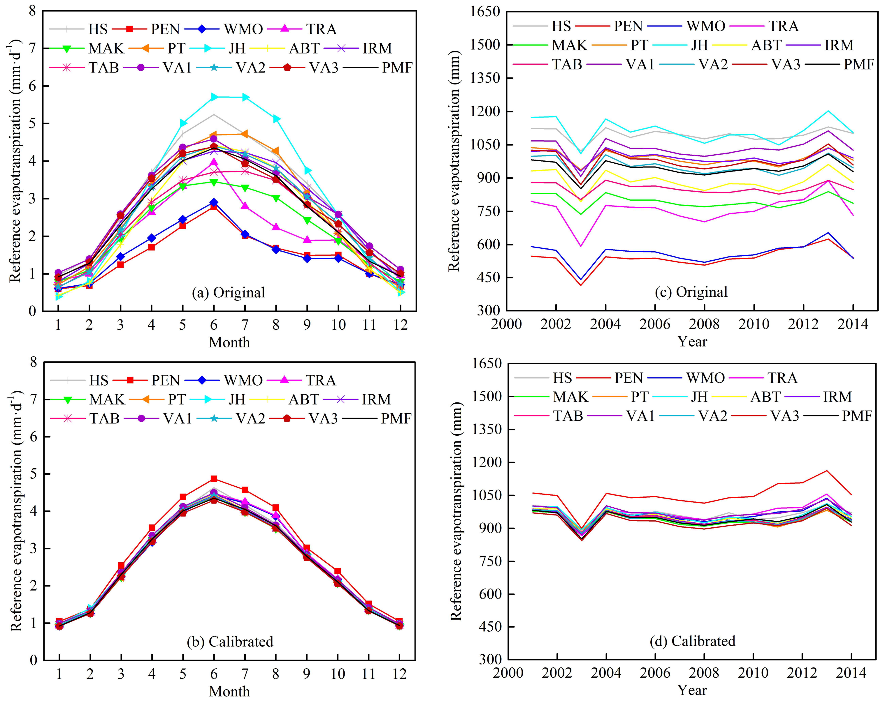
After the calibration, the reference evapotranspiration calculated by each of the 13 empirical models on monthly and annual timescales were very close to that estimated by the PMF-56 model, except for the PEN model, which overestimated the reference evapotranspiration from March to October and also on an annual timescale.

(5)

If the comprehensive meteorological datasets were available, the VA3 model would be the best alternative empirical model for the PMF-56 model, because it had an easy computation procedure and generated fewer errors compared to the other 12 empirical models, and it was also highly correlated with the PMF-56 model. After accurate validation for the VA3 model using Equation (5), the calibrated parameters of a and b for each site in the HRB were obtained. Based on data availability, the temperature-based, radiation-based, VA1, and VA2 models are recommended during April–October if corresponding input parameters in Table 2 are accessible in the HRB and other similar regions, whereas the mass transfer-based models are preferable in other months.

This study is a crucial contribution to the estimation of the ET₀ in the HRB, eastern China, when the large requirements of climate data cannot be met fully. The outcomes of this study will provide guidance to irrigation managers and agrometeorologists for the planning of water resources and irrigation scheduling in the HRB and other regions with similar climates, because the more accurate combination model will give an accurate and reliable estimation of the ET₀ based on the available comprehensive data.

References

1. Chu, R.; Li, M.; Shen, S.; Islam, A.R.M.T.; Cao, W.; Tao, S.; Gao, P. Changes in reference evapotranspiration and its contributing factors in Jiangsu, a major economic and agricultural province of eastern China. Water 2017, 9, 486. [Google Scholar] [CrossRef]
2. Tabari, H.; Kisi, O.; Ezani, A.; Talaee, P.H. SVM, ANFIS, regression and climate based models for reference evapotranspiration modeling using limited climatic data in a semi-arid highland environment. J. Hydrol. 2012, 444, 78–89. [Google Scholar] [CrossRef]
3. Wen, X.; Si, J.; He, Z.; Wu, J.; Shao, H.; Yu, H. Support-Vector-Machine-Based models for modeling daily reference evapotranspiration with limited climatic Data in extreme arid regions. Water Resour. Manag. 2015, 29, 3195–3209. [Google Scholar] [CrossRef]
4. Rahimikhoob, A.; Behbahani, M.R.; Fakheri, J. An Evaluation of Four Reference Evapotranspiration Models in a Subtropical Climate. Water Resour. Manag. 2012, 26, 2867–2881. [Google Scholar] [CrossRef]
5. Gocic, M.; Trajkovic, S. Software for estimating reference evapotranspiration using limited weather data. Comput. Electron. Agric. 2010, 71, 158–162. [Google Scholar] [CrossRef]
6. Allen, R.G.; Pereira, L.S.; Raes, D.; Smith, M. Crop Evapotranspiration-Guidelines for Computing Crop Water Requirements; FAO Irrigation and Drainage Paper 56; FAO: Rome, Italy, 1998. [Google Scholar]
7. Cai, J.; Liu, Y.; Lei, T.; Pereira, L.S. Estimating reference evapotranspiration with the FAO Penman-Monteith equation using daily weather forecast messages. Agric. For. Meteorol. 2007, 145, 22–35. [Google Scholar] [CrossRef]
8. Sentelhas, P.C.; Gillespie, T.J.; Santos, E.A. Evaluation of FAO Penman-Monteith and alternative methods for estimating reference evapotranspiration with missing data in Southern Ontario, Canada. Agric. Water Manag. 2010, 97, 635–644. [Google Scholar] [CrossRef]
9. Chen, D.; Gao, G.; Xu, C.-Y.; Guo, J.; Ren, G. Comparison of the Thornthwaite method and pan data with the standard Penman-Monteith estimates of reference evapotranspiration in China. Clim. Res. 2005, 28, 123–132. [Google Scholar] [CrossRef]
10. Huo, Z.; Feng, S.; Kang, S.; Dai, X. Artificial neural network models for reference evapotranspiration in an arid area of northwest China. J. Arid Environ. 2012, 82, 81–90. [Google Scholar] [CrossRef]
11. Liu, Y.; Yu, M.; Ma, X.; Xing, X. Estimating models for reference evapotranspiration with core meteorological parameters via path analysis. Hydrol. Res. 2016, 48, 340–354. [Google Scholar] [CrossRef]
12. Feng, Y.; Jia, Y.; Cui, N.; Zhao, L.; Li, C.; Gong, D. Calibration of Hargreaves model for reference evapotranspiration estimation in Sichuan basin of southwest China. Agric. Water Manag. 2017, 181, 1–9. [Google Scholar] [CrossRef]
13. Li, M.; Chu, R.; Shen, S.; Islam, A.R.M.T. Quantifying climatic impact on reference evapotranspiration trends in the Huai River Basin of eastern China. Water 2018, 10, 144. [Google Scholar] [CrossRef]
14. Mallikarjuna, P.; Jyothy, S.A.; Murthy, D.S.; Reddy, K.C. Performance of recalibrated equations for the estimation of daily reference evapotranspiration. Water Resour. Manag. 2014, 28, 4513–4535. [Google Scholar] [CrossRef]
15. Peng, L.; Li, Y.; Feng, H. The best alternative for estimating reference crop evapotranspiration in different sub-regions of mainland China. Sci. Rep. 2017, 7, 5458. [Google Scholar] [CrossRef] [PubMed]
16. Cobaner, M.; Citakoğlu, H.; Haktanir, T.; Kisi, O. Modifying Hargreaves-Samani equation with meteorological variables for estimation of reference evapotranspiration in Turkey. Hydrol. Res. 2016, 48, 480–497. [Google Scholar] [CrossRef]
17. Citakoglu, H.; Cobaner, M.; Haktanir, T.; Kisi, O. Estimation of monthly mean reference evapotranspiration in Turkey. Water Resour. Manag. 2014, 28, 99–113. [Google Scholar] [CrossRef]
18. Feng, Y.; Cui, N.; Zhao, L.; Hu, X.; Gong, D. Comparison of ELM, GANN, WNN and empirical models for estimating reference evapotranspiration in humid region of Southwest China. J. Hydrol. 2016, 536, 376–383. [Google Scholar] [CrossRef]
19. Mehdizadeh, S.; Behmanesh, J.; Khalili, K. Using MARS, SVM, GEP and empirical equations for estimation of monthly mean reference evapotranspiration. Comput. Electron. Agric. 2017, 139, 103–114. [Google Scholar] [CrossRef]
20. Chauhan, S.; Shrivastava, R.K. Performance evaluation of reference evapotranspiration estimation using climate based methods and artificial neural networks. Water Resour. Manag. 2009, 23, 825–837. [Google Scholar] [CrossRef]
21. George, B.A.; Reddy, B.R.S.; Raghuwanshi, N.S.; Wallender, W.W. Decision support system for estimating reference evapotranspiration. J. Irrig. Drain. Eng. 2002, 128, 1–10. [Google Scholar] [CrossRef]
22. Trajkovic, S. Comparison of radial basis function networks and empirical equations for converting from pan evaporation to reference evapotranspiration. Hydrol. Process. 2009, 23, 874–880. [Google Scholar] [CrossRef]
23. Sabziparvar, A.-A.; Tabari, H. Regional Estimation of Reference Evapotranspiration in Arid and Semiarid Regions. J. Irrig. Drain. Eng. 2010, 136, 724–731. [Google Scholar] [CrossRef]
24. Tabari, H.; Grismer, M.E.; Trajkovic, S. Comparative analysis of 31 reference evapotranspiration methods under humid conditions. Irrig. Sci. 2013, 31, 107–117. [Google Scholar] [CrossRef]
25. Bourletsikas, A.; Argyrokastritis, I.; Proutsos, N. Comparative evaluation of 24 reference evapotranspiration equations applied on an evergreenbroadleaved forest. Hydrol. Res. 2017. [Google Scholar] [CrossRef]
26. UNEP. World Atlas of Desertification, 2nd ed.; United Nations Environment Programme: London, UK, 1997; 182p. [Google Scholar]
27. Todorovic, M.; Karic, B.; Pereira, L.S. Reference evapotranspiration estimate with limited weather data across a range of Mediterranean climates. J. Hydrol. 2013, 481, 166–176. [Google Scholar] [CrossRef]
28. Shiri, J.; Nazemi, A.H.; Sadraddini, A.A.; Landeras, G.; Kisi, O.; Fard, A.F.; Marti, P. Comparison of heuristic and empirical approaches for estimating reference evapotranspiration from limited inputs in Iran. Comput. Electron. Agric. 2014, 108, 230–241. [Google Scholar] [CrossRef]
29. Estévez, J.; Gavilán, P.; Berengena, J. Sensitivity analysis of a Penman-Monteith type equation to estimate reference evapotranspiration in southern Spain. Hydrol. Process. 2009, 23, 3342–3353. [Google Scholar] [CrossRef]
30. Dinpashoh, Y.; Jhajharia, D.; Fakheri-Fard, A.; Singh, V.P.; Kahya, E. Trends in reference crop evapotranspiration over Iran. J. Hydrol. 2011, 399, 422–433. [Google Scholar] [CrossRef]
31. Jhajharia, D.; Dinpashoh, Y.; Kahya, E.; Singh, V.P.; Fakheri-Fard, A. Trends in reference evapotranspiration in the humid region of northeast India. Hydrol. Process. 2012, 26, 421–435. [Google Scholar] [CrossRef]
32. Hargreaves, G.H.; Samani, Z.A. Reference crop evapotranspiration from temperature. Appl. Eng. Agric. 1985, 1, 96–99. [Google Scholar] [CrossRef]
33. Penman, H.L. Natural evaporation from open water, bare soil and grass. Proc. R. Soc. A Math. Phys. 1948, 193, 120–145. [Google Scholar] [CrossRef]
34. World Meteorological Organization (WMO). Measurement and Estimation of Evaporation and Evapotranspiration; Technical Paper (CIMO-Rep); WMO: Geneva, Switzerland, 1966; Volume 83. [Google Scholar]
35. Trabert, W. Neue Beobachtungen uber Verdampfungsgeschwindigkeiten. Meteorol. Z. 1896, 13, 261–263. [Google Scholar]
36. Makkink, G.F. Testing the Penman formula by means of lysimeters. J. Inst. Water Eng. 1957, 11, 277–288. [Google Scholar]
37. Priestley, C.H.B.; Taylor, R.J. On the assessment of surface heat flux and evaporation using large-scale parameters. Mon. Weather Rev. 1972, 100, 81–92. [Google Scholar] [CrossRef]
38. Jensen, M.E.; Haise, H.R. Estimating evapotranspiration from solar radiation. J. Irrig. Drain. Div. 1963, 89, 15–41. [Google Scholar]
39. Abtew, W. Evapotranspiration measurements and modeling for three wetland systems in South Florida. J. Am. Water Resour. Assoc. 1996, 32, 465–473. [Google Scholar] [CrossRef]
40. Irmak, S.; Irmak, A.; Allen, R.G.; Jones, J.W. Solar and net radiation-based equations to estimate reference evapotranspiration in humid climates. J. Irrig. Drain. Eng. 2003, 129, 336–347. [Google Scholar] [CrossRef]
41. Valiantzas, J.D. Simple ET0 forms of Penman’s equation without wind and/or humidity data. I: Theoretical development. J. Irrig. Drain. Eng. 2013, 139, 1–8. [Google Scholar] [CrossRef]
42. Valiantzas, J.D. Simple ET0 forms of Penman’s equation without wind and/or humidity data. II: Comparisons with reduced set-FAO and other methodologies. J. Irrig. Drain. Eng. 2013, 139, 9–19. [Google Scholar] [CrossRef]
43. Samaras, D.A.; Reif, A.; Theodoropoulos, K. Evaluation of Radiation-Based reference evapotranspiration models under different Mediterranean climates in central Greece. Water Resour. Manag. 2014, 28, 207–225. [Google Scholar] [CrossRef]
44. Mann, H.B. Nonparametric test against trend. Econometrica 1945, 13, 245–259. [Google Scholar] [CrossRef]
45. Kendall, M.G. Rank Correlation Methods; Griffin: London, UK, 1975. [Google Scholar]
46. Sen, P.K. Estimates of the Regression Coefficient Based on Kendall’s Tau. J. Am. Stat. Assoc. 1968, 63, 1379–1389. [Google Scholar] [CrossRef]
47. Theil, H. A Rank Invariant Method of Linear and Polynomial Regression Analysis; North-Holland Publishing Co.: Amsterdam, The Netherlands, 1950. [Google Scholar]
48. Li, M.; Chu, R.; Shen, S.; Islam, A.R.M.T. Dynamic analysis of pan evaporation variations in the Huai River Basin, a climate transition zone in eastern China. Sci. Total Environ. 2018, 625, 496–509. [Google Scholar] [CrossRef] [PubMed]
49. Zhang, K.; Pan, S.; Zhang, W.; Xu, Y.; Cao, L.; Hao, Y.; Wang, Y. Influence of climate change on reference evapotranspiration and aridity index and their temporal-spatial variations in the Yellow River Basin, China, from 1961 to 2012. Quat. Int. 2015, 380, 75–82. [Google Scholar] [CrossRef]
50. Zheng, C.; Wang, Q. Spatiotemporal variations of reference evapotranspiration in recent five decades in the arid land of Northwestern China. Hydrol. Process. 2014, 28, 6124–6134. [Google Scholar] [CrossRef]
51. Song, X.; Zhu, K.; Lu, F.; Xiao, W. Spatial and temporal variation of reference evapotranspiration under climate change: A case study in the Sanjiang Plain, Northeast China. Hydrol. Res. 2017, 49, 251–265. [Google Scholar] [CrossRef]
52. Ahooghalandari, M.; Khiadani, M.; Jahromi, M.E. Developing equations for estimating reference evapotranspiration in Australia. Water Resour. Manag. 2016, 30, 3815–3828. [Google Scholar] [CrossRef]
53. Djaman, K.; Irmak, S.; Futakuchi, K. Daily reference evapotranspiration estimation under limited data in eastern Africa. J. Irrig. Drain. Eng. 2016, 143, 1–13. [Google Scholar] [CrossRef]
54. Ahooghalandari, M.; Khiadani, M.; Jahromi, M.E. Calibration of Valiantzas’ reference evapotranspiration equations for the Pilbara region, Western Australia. Theor. Appl. Climatol. 2017, 128, 845–856. [Google Scholar] [CrossRef]
55. Irmak, S.; Payero, J.O.; Martin, D.L.; Irmak, A.; Howell, T.A. Sensitivity analyses and sensitivity coefficients of standardized daily ASCE-Penman-Monteith equation. J. Irrig. Drain. Eng. 2006, 132, 564–578. [Google Scholar] [CrossRef]
56. Jensen, M.E.; Burman, R.D.; Allen, R.G. Evapotranspiration and Irrigation Water Requirements: A Manual; ASCE Manuals and Reports on Engineering Practice, No. 70; ASCE: New York, NY, USA, 1990. [Google Scholar]
57. Tegos, A.; Malamos, N.; Koutsoyiannis, D. A parsimonious regional parametric evapotranspiration model based on a simplification of the Penman-Monteith formula. J. Hydrol. 2015, 524, 708–717. [Google Scholar] [CrossRef]
58. Tegos, A.; Malamos, N.; Efstratiadis, A.; Tsoukalas, I.; Karanasios, A.; Koutsoyiannis, D. Parametric Modelling of Potential Evapotranspiration: A Global Survey. Water 2017, 9, 795. [Google Scholar] [CrossRef]
59. Trajkovic, S.; Kolakovic, S. Wind-adjusted Turc equation for estimating reference evapotranspiration at humid European locations. Hydrol. Res. 2009, 40, 45–52. [Google Scholar]
Figure 1. Map showing the geographical location of the meteorological stations in the Huai River Basin (HRB). Note: The red line is the boundary between the sub-humid (I) and humid (II) regions.
Water 10 00493 g001
Figure 2. Box plot showing the monthly ETPMF in the HRB. Boxes and whiskers represent the interquartile range (between the 25th and 75th percentiles) and the maximum and minimum values; the central red solid line represents the median, and the hollow circle represents the average value.
Water 10 00493 g002
Figure 3. Spatial distribution of monthly ETPMF in the HRB during 1961–2014. Note: Jan, Feb, Mar, Apr, May, Jun, Jul, Aug, Sep, Oct, Nov, and Dec are the abbreviations of January, February, March, May, June, July, August, September, October, November, and December, respectively. (al) represent the ETPMF from January to December respectively.
Water 10 00493 g003
Figure 4. Spatial distribution of monthly ETPMF trends in the HRB during 1961–2014. Note: Jan, Feb, Mar, Apr, May, Jun, Jul, Aug, Sep, Oct, Nov, and Dec are the abbreviations of January, February, March, May, June, July, August, September, October, November, and December, respectively. The solid rhombus and cross-shaped signs represent the decreasing and increasing trends with a significance level of less than 0.05. (al) represent the trends of ETPMF from January to December respectively.
Water 10 00493 g004
Figure 5. Comparative analysis of the daily reference evapotranspiration estimated by the standardized PMF-56 model (ETPMF, x axis) against the 13 empirical models (ETEMP, y axis). The red dashed line indicates the linear fit of the scatters; the solid line represents the 1:1 line. The sample size is 19,723.
Water 10 00493 g005
Figure 6. Comparison of the monthly ETEMP and ETPMF in the HRB during 1961–2014.
Water 10 00493 g006
Figure 7. Radar charts showing the comparison of the RRMSE values between the original reference evapotranspiration and the calibrated reference evapotranspiration using the 13 empirical models in the HRB from 2001 to 2014. Note: Jan, Feb, Mar, Apr, May, Jun, Jul, Aug, Sep, Oct, Nov, and Dec are the abbreviations of January, February, March, May, June, July, August, September, October, November, and December, respectively.
Water 10 00493 g007
Figure 8. Radar charts showing the comparison of the MAE values between the original reference evapotranspiration and the calibrated reference evapotranspiration using the 13 empirical models in the HRB from 2001 to 2014. Note: Jan, Feb, Mar, Apr, May, Jun, Jul, Aug, Sep, Oct, Nov, and Dec are the abbreviations of January, February, March, May, June, July, August, September, October, November, and December, respectively.
Water 10 00493 g008
Figure 9. Radar charts showing the comparison of the NS values between the original reference evapotranspiration and the calibrated reference evapotranspiration using the 13 empirical models in the HRB from 2001 to 2014. Note: Jan, Feb, Mar, Apr, May, Jun, Jul, Aug, Sep, Oct, Nov, and Dec are the abbreviations of January, February, March, May, June, July, August, September, October, November, and December, respectively.
Water 10 00493 g009
Figure 10. Comparison of the original reference evapotranspiration and the calibrated reference evapotranspiration on monthly and annual timescales. (a,b) are original and calibrated reference evapotranpiration on monthly timescale respectively; (c,d) are original and calibrated reference evapotranpiration on annual timescale respectively.
Water 10 00493 g010