Using a Hydrological Model to Simulate the Performance and Estimate the Runoff Coefficient of Green Roofs in Semiarid Climates

Abstract

Green roofs offer a series of benefits to buildings and to the urban environment. Their use in dry climates requires optimizing the choice of their components (i.e., vegetation, substrate and drainage layer) for the specific local climatic conditions, in order to minimize irrigations needs while preserving the attributes of the roof. In this study, we calibrated and validated an existing hydrological model—IHMORS—for the simulation of the hydrological performance of green roofs. Simulated results were compared to experimental data obtained in an outdoor test facility on several green roof specimens, representing a variety of green roofs configurations. IHMORS was able to reasonably predict the soil moisture dynamics for all tested specimens. The specimens of 10 cm depth were the best simulated by the model, while some overestimation was observed during the model validation for the 5 and 20 cm depth specimens. The model was then used to estimate the number of days in which irrigation is needed, as well as analyze the water runoff control performance of all specimens. We related the amount of water retained by the substrate and depth, magnitude and intensity of precipitation event, and the initial substrate moisture. For all events, the lowest runoff coefficient was simulated for the 20 cm specimens. Our study showed the full potential of the model for estimating the water needs and the runoff control performances of different variants of green roofs.

1. Introduction

Green roofs are a type of green infrastructure technology that has been incorporated into the design and construction of buildings because of the benefits they offer to the buildings themselves and to the urban environment. Some of these benefits include the reduction of the heating and cooling consumption of buildings, the mitigation of the urban heat island effect, the enhancements in urban biodiversity, the improvement of the air and water quality and the stormwater runoff control by lowering and delaying the peak water runoff [1,2,3,4]. In fact, green roofs are part of the techniques classified as ‘sustainable urban drainage systems’, offering a solution to the reduction of the surface storage capacity in cities due to the growing urban development. Unlike traditional drainage infrastructures, these systems preserve and recreate the natural landscape features to treat storm water as a resource rather than a waste [3]. They are able to infiltrate precipitation and collect runoff from impervious surfaces, with the retained volume then being redistributed to other layers and/or eventually evapotranspired.

In the last two decades, there has been a substantial expansion of green roof technologies in humid and temperate climates [5]. Nonetheless, green roofs are nowadays used and studied in Mediterranean and semiarid climates, although in a more limited manner (e.g., [5,6,7,8,9]). Water requirements of green roofs in these climates can be significant, and irrigation is usually unavoidable for plant survival during prolonged dry periods [5]. Maintaining the vegetation in these climates without using a large amount of water for irrigation is really challenging [10]. Thus, it is of great importance to understand the hydrological perform of green roofs and develop and exhaustively test models that can be used to analyze and design their constituents in order to minimize water requirements. In particular, the simulation of (1) surface/subsurface processes and (2) the continuous dynamics of the soil water content controlled by evapotranspiration and irrigation are essential to study the performance of green infrastructure and evaluate plant survival and the overall sustainability of drainage techniques in arid and semiarid regions [11,12].

Long-term field monitoring of the hydrologic behavior and performances of green roofs is costly and work intensive and is not appropriate to individually study each factor impacting the performance of the roof. Moreover, laboratory experiments cannot easily reproduce the real variation of the climatic parameters [13]. Modeling offers an interesting alternative to address these issues, for both assessment and design purposes. Nonetheless, there are only few models that can accurately estimate the moisture transfer occurring in the different layers of green roofs and the resulting water content, taking into account possible runoff from other pervious or impervious areas [14,15]. As example, several researchers have used HYDRUS-1D software to model the substrate water transport in order to evaluate the storm water response of green roofs [16,17,18,19]. Regrettably, this software cannot simulate constructional elements like drainage layers, so it can be unrepresentative of reality [15,16]. Other models like SWAP (Soil, Water, Atmosphere and Plant) and SWMS-2D (Variably-Saturated Two-Dimensional Water Flow and Transport Model) are not able to simulate complex systems with drainages or connections to neighboring areas. SWMM (Storm Water Management Model) is not capable of analyzing green roof hydrologic features based on design parameters [20] and also presents other weaknesses as explained in [14].

Most of the existing models have not been validated with experimental data measured on a complete variety of green roof systems and designs during a long and representative test period. As an example, [13] used a simple hydrologic model based on water balance and a conventional potential evapotranspiration model to predict the moisture content of green roofs, with simulation results compared with field measurements. However, this investigation was focused on dry periods without any precipitation, irrigation and runoff. Ref. [16] evaluated the storm water response for different substrate depths of green roofs, but only on the basis of simulations. Other studies used a very limited number of tested configurations (1 to 3) for the validation of the green roof model [19,20,21]. In order to overcome the limitations of the HYDRUS model, [19] developed a new hydrological model by coupling a substrate layer (HYDRUS-1D model) with a storage layer in order to predict the irrigation requirement of green roofs. However, this model was validated with the measured data carried out on only one pilot green roof. Finally, most of the validated models were usually proven for humid regions, where local materials and climatic conditions greatly differ from those of arid and semiarid climates [22,23].

This paper presents the application of a recently developed hydrological model—the IHMORS model—to different green roof configurations under semiarid climatic conditions. Our objective is to evaluate the capability of this model with a large number of green roof specimens differing mainly in their substrate depths and drainage systems in order to address the above-mentioned limitations of current models used with green roofs. IHMORS is capable of simulating the different hydrological surface and subsurface processes taking place in green infrastructure and continuously estimates the water content of the substrate for each moment of the year, as well as the irrigation needs, and the runoff performance [14]. To achieve this goal, the model was calibrated and validated with data from an extensive test campaign carried out on 10 different green roof specimens exposed to real outdoor conditions during several months in a test facility located in Santiago, Chile. Furthermore, the validated model is then used to estimate the number of days for which irrigation is needed, as well as the control runoff performance of each specimen.

2. Materials and Methods

2.1. Experimental Set-Up

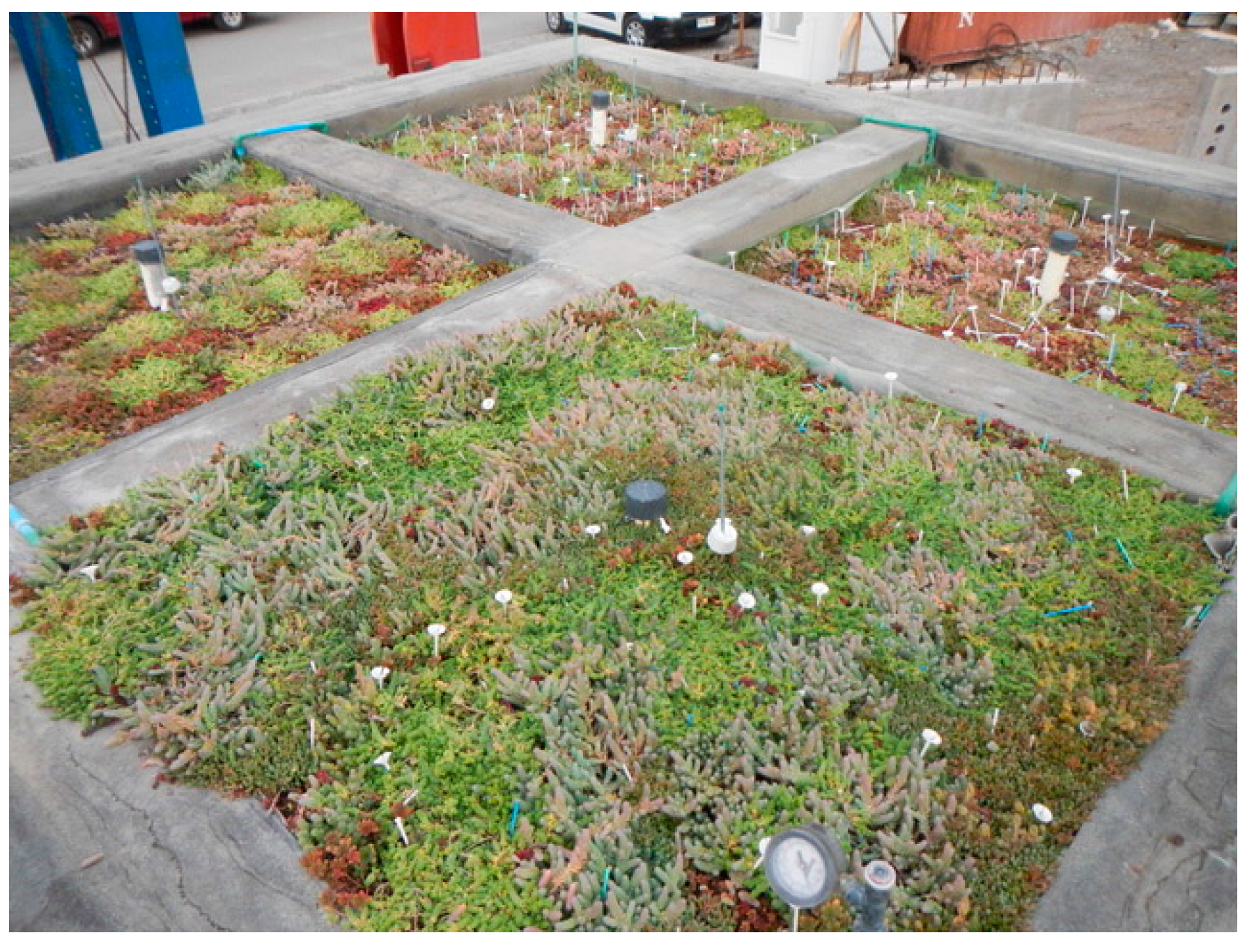
2.1.1. Test Facility

A long-term experiment was conducted during the period 2014–2015 in a test facility called ‘Laboratory of Vegetative Infrastructure of Buildings’ (LIVE, for its acronym in Spanish). The laboratory is located in Santiago, Chile (33°26′ S, 70°39′ W) at the Pontificia Universidad Católica de Chile [5]. Santiago is a city where more than 50,000 m² of green roofs and walls have been implemented in recent years [9], which is characterized by a typical dry Mediterranean climate (semiarid) with warm temperate climate and dry summers [24]. The average annual temperature is 14.6 °C and the mean annual precipitation is 313 mm, with 25–30 rainy days per year [25].

The LIVE consists of 4 testing modules of 2 m height, with a high level of thermal insulation in their walls and floors. Three of the modules are 25 m²; each while one is 35 m². The roofing system of three modules was a concrete slab while the remaining module was built with a steel roof deck. This facility allows testing of up to 18 different specimens of green roofs. In the context of this study, 12 green roof specimens were installed and tested; each one has an area of about 1.8 m × 1.8 m (see Figure 1).

2.1.2. Description of Tested Green Roofs Specimens

All specimens have the same substrate and the same vegetation. The substrate used was a commercial substrate with sandy loam texture (68% sand, 20% silt and 12% clay), which is commonly used for green roofs [26]. The vegetation is a mixture of seven species of sedum: S. spurium, S. kamtschaticum, S. reflexum, S. sexangulare, S. album, S. hybridum and S. rupestre [27].

The specimens were constructed with different slopes, depths and drainage systems [5]. We classified them according to their common characteristics in 5 groups as indicated in

Table 1. Characteristics of each tested green roof specimen. Each specimen of a given group is identified with letters a, b or c.

Group	ID	Drainage System	Slope (%)	Substrate Depth (cm)
G5	G5a	Sika® Sarnavert Aquadrain	2	5
	G5b	Vydro®	2	5
G10	G10a	Sika® Sarnavert Aquadrain 550	2	10
	G10b	Delta®-Drain	2	10
	G10c	Vydro®	2	10
G20	G20a	N/A (Recycled)	2	20
	G20b	Delta®-Floraxx	2	20
G10s	G10sa	Delta®-Floraxx	2	10
	G10sb	Delta®-Floraxx	2	10
	G10sc	Delta®-Floraxx	2	10
G10w	G10wa	--	1	10
	G10wb	--	5	10

: G5, G10 and G20 are specimens with a layer of 5, 10 and 20 cm depth, respectively, which have different drainage systems. Each specimen of a given group is identified with a letter (i.e., a, b or c). G10w are specimens with a layer of 10 cm depth but without a drainage layer. Finally, the group G10s corresponds to three replicas of the same specimen, with a layer of 10 cm depth and the same drainage system. These 3 replicas provided an estimate and control of the variability. The construction and instrumentation costs of the test facility explain the lack of replicates for the other groups. Nevertheless, the area of each specimen (~3.3 m²) was expected to reduce the border condition effects and provide representative measurements. More details about the test facility and the specimens can be found in [5].

2.1.3. Monitoring

For each green roof specimen, the volumetric water content (VWC) of the substrate was continuously measured with a sensor (GS3, Decagon Devices) installed at mid-height of the layer. All meteorological data were collected from a weather station installed on the roof. The station has a series of high-resolution sensors for recording temperature and relative air humidity (EHT, Decagon Devices), wind speed and direction (Davis Cup, Decagon Devices, Pullman, WA, USA), precipitation (ECRN-100, Decagon Devices, Pullman, WA, USA) and PAR-radiation (QSO-S, Decagon Devices, Pullman, WA, USA). All sensors were connected to a data acquisition system and were recorded every 5 min.

2.2. Modeling

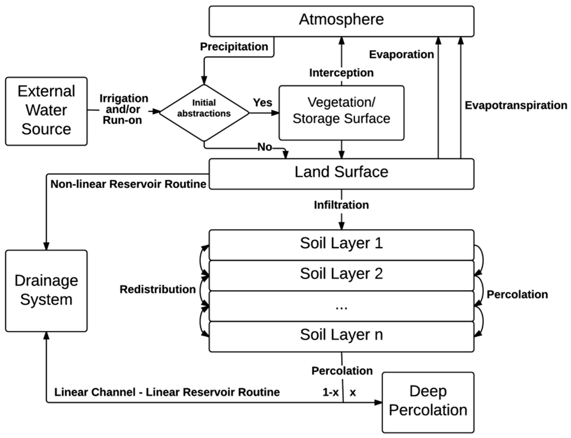
2.2.1. Hydrological Model

IHMORS (Integrated Hydrological Model at Residential Scale) was the model used to simulate green roof performance. This model continuously simulates the rainfall-runoff processes at a residential scale, focusing on the performance of storm water runoff control facilities, as well as irrigation practices [14]. To simulate common urban drainage techniques such as green roofs, the model combines and connects different subareas which can be permeable or impermeable. Each permeable subarea can be represented through a series of layers. As indicated in Figure 2, each subarea is subject to different surface processes (i.e., interception, evapotranspiration and infiltration) and subsurface processes (percolation and redistribution). IHMORS combines equations that represent these biophysical and hydrological processes—which are presented in [14]—with a mass balance equation to obtain the dynamics of the substrate moisture and the surface and subsurface hydrograph. To solve the mass balance, the model assumes that the substrate moisture is constant throughout each layer. This assumption is valid when the storm water facility is composed of thin layers, such as in green roofs [13]. Overall, we adopted IHMORS because of its novelty and specific capabilities, as it can explicitly simulate relevant processes in semiarid and Mediterranean environments, such bare soil evaporation, subsurface runoff hydrographs and soil moisture redistribution. IHMORS cannot simulate lateral subsurface flow; this limitation is assumed to not be relevant for our application, but it deserves to be studied in the future.

2.2.2. Assumptions

In the framework of this study, a certain number of assumptions and simplifications were made compared to the full potential of the IHMORS model. Each green roof specimen was modeled with a unique permeable substrate layer without any connections to other permeable or impermeable neighboring areas. The drainage layer was explicitly modeled only for the specimen G5^b because the drainage layer used (Vydro^®) is highly absorbing, similar to a sponge, with a clear effect on the water content of the thin substrate layer (only 5 cm) above. For the other specimens, a preliminary analysis showed a limited impact of the drainage layer on the substrate characteristics and performance. Therefore, for simplicity, it was decided not to model them.

As one of the aims of the study is to analyze the irrigation needs, all experiments were carried out without any irrigation. This is why all simulations were made without any irrigation as well. In fact, the calibration period of this study corresponds to the rainy season of year 2014, between 29 June and 15 October, whereas the validation period corresponds to the rainy season of year 2015, between 17 June and 17 September.

2.2.3. Inputs and Outputs

The inputs required by IHMORS include: (1) weather; (2) time step information and (3) physical properties of each area including vegetation properties. The weather data were collected from the weather station (see Section 2.1.3). The majority of them were directly used to calculate the evapotranspiration according to the Penman-Monteith method used by the model [28]. The net solar radiation was estimated from the PAR-radiation according to [28]. The time step for the simulations was the same as that used for the measurements of the weather data (5 min).

All green roof specimens share most of the substrate parameters needed to simulate the water flow through the substrate. The majority of them were determined by laboratory experiments using the method described in [26].

Table 2. Substrate parameters common to all specimens. ${\theta }_r$ is the residual substrate water content, ${\theta }_s$ is the saturated substrate water content, $n$ is the curve share parameter, $L$ is the empirical pore tortuosity, $K_s$ is the saturated hydraulic conductivity, $\psi$ is the bubbling pressure, ${\theta }_{WP}$ is the wilting point, $d_{REW}$ is the readily evaporated water, $K_{cmax}$ is the maximum crop coefficient and $\beta$ is the adjustment coefficient of the second stage of evaporation.

Parameter	Value	Units
${\theta }_r$	0.010	m3 m−3
${\theta }_s$	0.637	m3 m−3
$n$	1.44	--
$L$	0.5	--
$K_s$	145.1	mm h−1
$\psi$	85.5	mm
${\theta }_{WP}$	0.15	m3 m−3
$d_{REW}$	11	mm
$K_{cmax}$	2.180	--
$\beta$	0.540	--

shows these parameters where ${\theta }_r$ is the residual substrate water content, ${\theta }_s$ is the saturated substrate water content, $n$ is the curve shape parameter (Van Genuchten model), $L$ is the empirical pore tortuosity, $K_s$ is the saturated hydraulic conductivity, $\psi$ is the bubbling pressure, ${\theta }_{WP}$ is the wilting point, $d_{REW}$ corresponds to the readily evaporated water, $K_{cmax}$ is the maximum crop coefficient and $\beta$ is the adjustment coefficient of the second stage of evaporation. The last three parameters, used in evaporation process, were obtained from the experimental data as explained in [14]. There are two other substrate-related parameters, the initial water content and the water content at field capacity, that were estimated from observed data collected during the calibration phase, so they are different for each specimen (see Section 3.1). Further details about the mathematical representation of the different processes in IHMORS and the role of the previous parameters can be obtained from the original publication [14].

Four parameters related to the vegetation (evapotranspiration and interception processes) were determined. The crop coefficient ($K_c$) and the leaf area index ($k$) were estimated from literature review: $K_c$ = 0.53 [29] and $k$ = 3 [28]. The vegetation coverage ($V_c$) was measured on-site whereas the maximum interception capacity (S) was obtained by a calibration process based on observed data collected during the calibration phase. This was done because, due to its conceptual character, this parameter cannot be measured by laboratory tests.

The IHMORS model produces several outputs such as the VWC of each layer for each time step, the outflow hydrograph and the substrate water content duration (SWCD) curve. This last curve proposed by [14] corresponds to the graphical representation of the percentage of time the VWC exceeds a given value. Furthermore, a detailed report with a mass balance for each layer is produced: a surface balance with all inflows (rainfall, runon, irrigation) and outflows (interception, infiltration, runoff) and a subsurface balance for each layer with all inflows and outflows as well (infiltration, percolation and redistribution to neighboring layers, etc.).

2.3. Data Analysis

In order to assess the level of agreement between the simulation results and the measured data both for the calibration and validation periods, two metrics were used: the Modified Coefficient of Efficiency (MCE) and the Mean Absolute Error (MAE), given by [30]:

$$\mathrm{MCE}=1-\frac{{\sum }_i|O_i-E_i|}{{\sum }_i|O_i-\overline{O}|}$$

(1)

$$\mathrm{MAE}=N^{-1}{{\displaystyle \sum }}_i|O_i-E_i|$$

(2)

where $O_i$ and $E_i$ are the observed and simulated data, respectively, $\overline{O}$ is the observed mean and N is the total number of observations and simulations. MAE is an example of a residual measure, which is by far the most prevalent measure for model evaluation as it calculates the difference between observed and modelled data points in the units of the variable [30]. Additionally, the MCE is a relative error measure to test the ability of the model to preserve the pattern of observed data [30]. Indeed, Legates and McCabe [31] suggest that MCE is the most appropriate relative error measure, which combines the correlation coefficient and the observed and simulated means (μ) and standard deviations (σ) [30].

3. Results

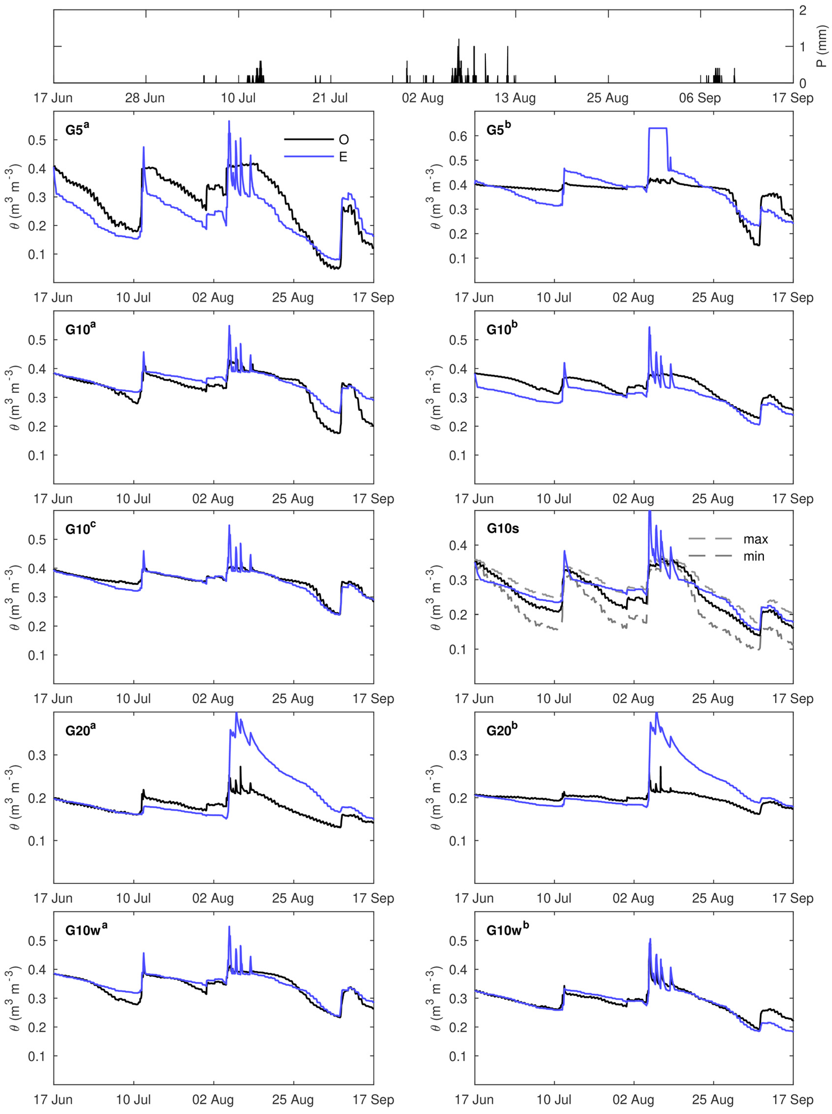
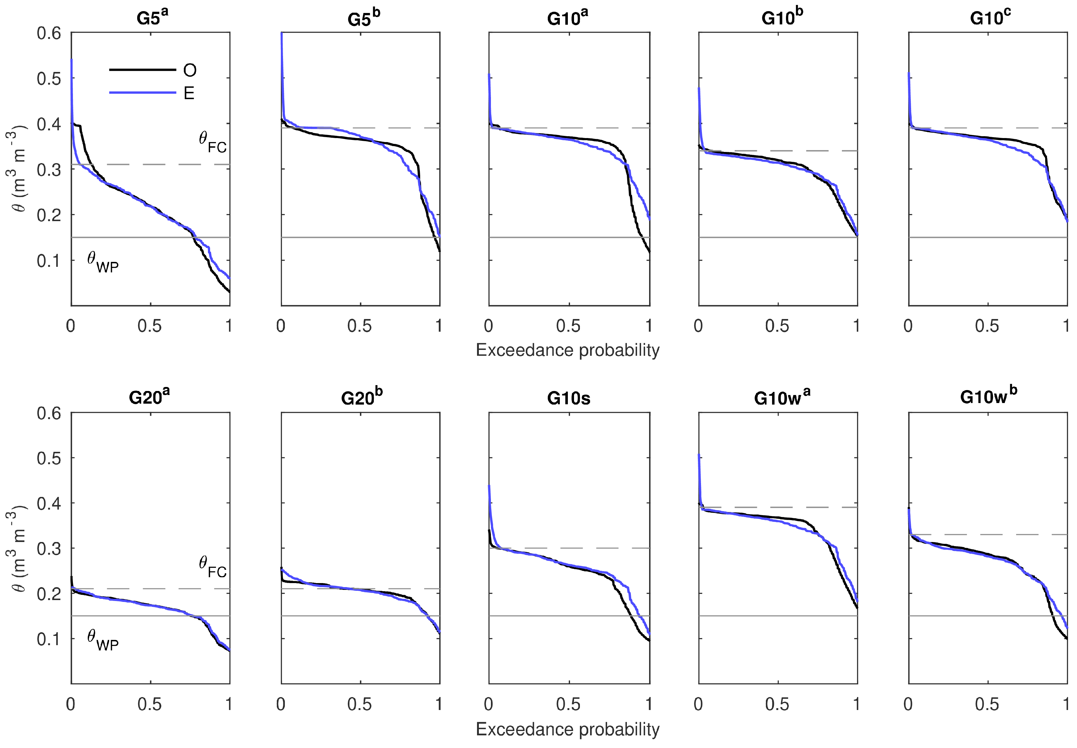
3.1. Calibration and Validation of the Model

3.1.1. Calibration Phase

During this phase, the parameter S was calibrated by minimizing the error between the measured and the simulated data of the VWC of the substrate of each green roof specimen. Ten rainfall events occurred during this period, accumulating 136.8 mm (Figure 3 upper). The three largest events occurred on 14 July (35.6 mm), 6 August (15.6 mm) and 23 August (35.2 mm). No irrigation was implemented during this time.

The observed data were also used to estimate the field capacity ${\theta }_{FC}$ for each specimen. This value corresponds to the substrate moisture recorded after a sharp drop during rainy events in the VWC vs. time plot. At this point, water stops draining because of gravity [32]. This value was quite constant during the rainfall period of 2014 (see observed data in Figure 3) although it was very different among the different specimens and especially among the groups. This probably occurs as a consequence of the variability in the substrate structure generated during the construction and the development and dynamics of the vegetation. Finally, the initial water content ${\theta }_i$was taken as the first record of the data set.

All evaluated values are shown in

Table 3. Evaluated parameters for each specimen: ${\theta }_i$is the initial substrate moisture, ${\theta }_{FC}$ is the field capacity, $V_c$is the vegetation coverage and S is the maximum interception capacity.

Group	ID	Substrate		Vegetation
		${\mathit{\theta }}_{\mathit{i}}$ (m3 m−3)	${\mathit{\theta }}_{\mathit{F}\mathit{C}}$ (m3 m−3)	${\mathit{V}}_{\mathit{c}}$ (%)	S (mm)
G5	G5a	0.228	0.31	56.6	7.8
	G5b	0.368	0.39	73.1	20
G10	G10a	0.371	0.39	85.3	8.3
	G10b	0.333	0.34	90.7	11.3
	G10c	0.371	0.39	82.9	7
G20	G20a	0.175	0.21	95.7	50
	G20b	0.220	0.21	95.7	44.4
G10s	G10s	0.261	0.30	81.4	13.9
G10w	G10wa	0.370	0.39	84.2	7.7
	G10wb	0.299	0.33	84.2	38.3

. Since specimens in the G10s group have the same constructional features (Table 1), a single specimen was modeled and compared using the average measured data of the 3 G10s specimens.

Figure 3 shows the simulated (estimated) and measured (observed) substrate moisture curve during the whole calibration period, for each specimen. The maximum and minimum measured data for G10s specimens are also given.

Table 4. MCE, MAE, mean (μ) and standard deviation (σ) from observed (O) and estimated (E) volumetric water content (VWC) during calibration period (rainy season 2014).

Group	ID	MCE	MAE	$\mathit{\mu }$ (VWC)		$\mathit{\sigma }$ (VWC)
				O	E	O	E
G5	G5a	0.76	0.02	0.212	0.211	0.091	0.074
	G5b	0.56	0.02	0.342	0.355	0.064	0.060
G10	G10a	0.64	0.02	0.343	0.348	0.070	0.047
	G10b	0.71	0.01	0.299	0.299	0.049	0.044
	G10c	0.69	0.01	0.352	0.346	0.049	0.049
G20	G20a	0.66	0.01	0.164	0.165	0.034	0.033
	G20b	0.64	0.01	0.201	0.200	0.026	0.028
G10s	G10s	0.65	0.02	0.244	0.255	0.058	0.049
G10w	G10wa	0.73	0.01	0.342	0.342	0.056	0.048
	G10wb	0.76	0.01	0.265	0.267	0.059	0.049

shows the goodness-of-fit coefficient for each specimen, while μ and σ from observed (O) and estimated (E) data are also presented.

As can be seen, there is a very good agreement between the observed and predicted data. The average value of MCE is 0.68. In all cases, the MAE is lower than the standard deviation. MCE values differ according to the type of drainage system and the layer depth. MCE values from specimens with 10 cm depth (G10, G10s and G10w) are on average slightly higher than 20 cm specimens (G20). Moreover, all specimens except G5^b have MCE values higher than 0.64. The reason why the value for G5^b is lower is explained by the fact that this layer is very thin (only 5 cm) and has a drainage system similar to a sponge, which is quite complex to model. In fact, the performance of the other 5 cm depth specimen G5^a is better (i.e., MCE of 0.76) because its drainage layer (Sika^® Sarnavert Aquadrain, Table 1), which was not simulated explicitly, does not affect the performance of the substrate. On the other hand, G10w specimens have higher MCE values, probably because they do not have any drainage layer which prevents an influence of other factors in the calibration process of the S parameter. The moisture curves for the different specimens are analyzed in more detail during the second measurement period (see Section 3.1.2).

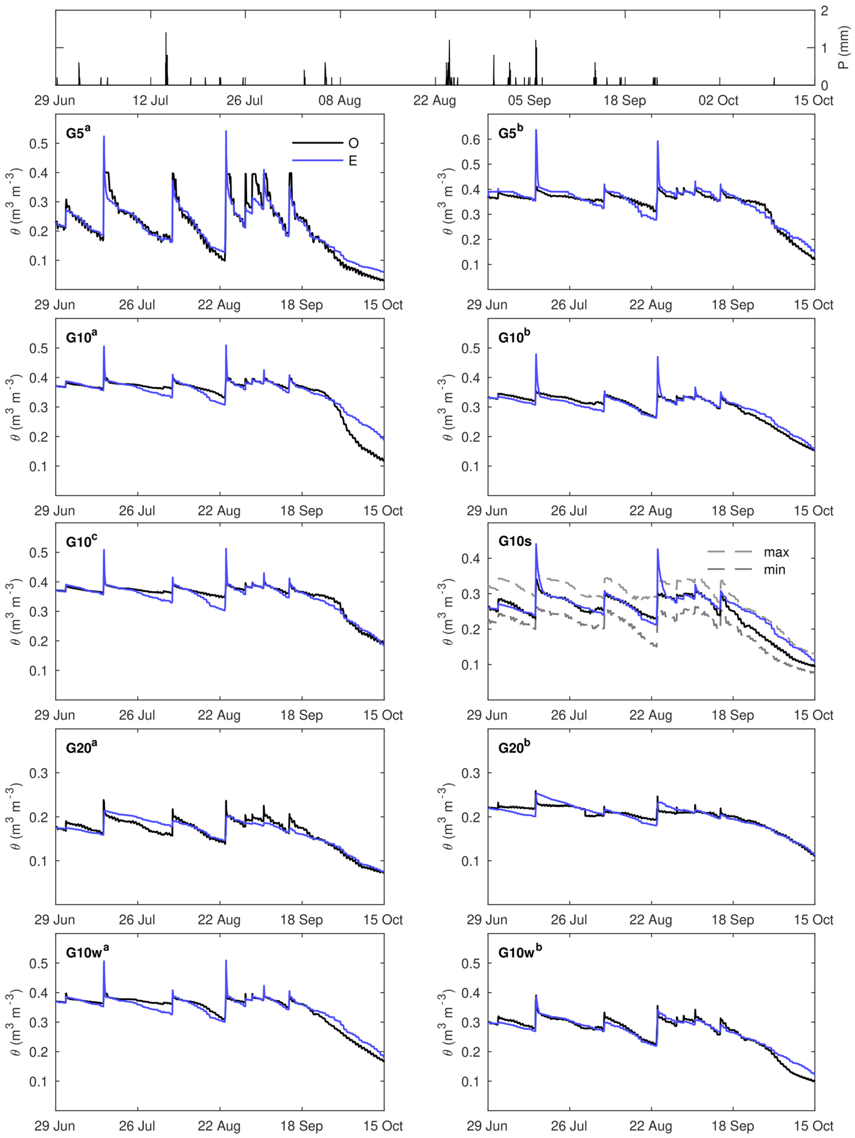
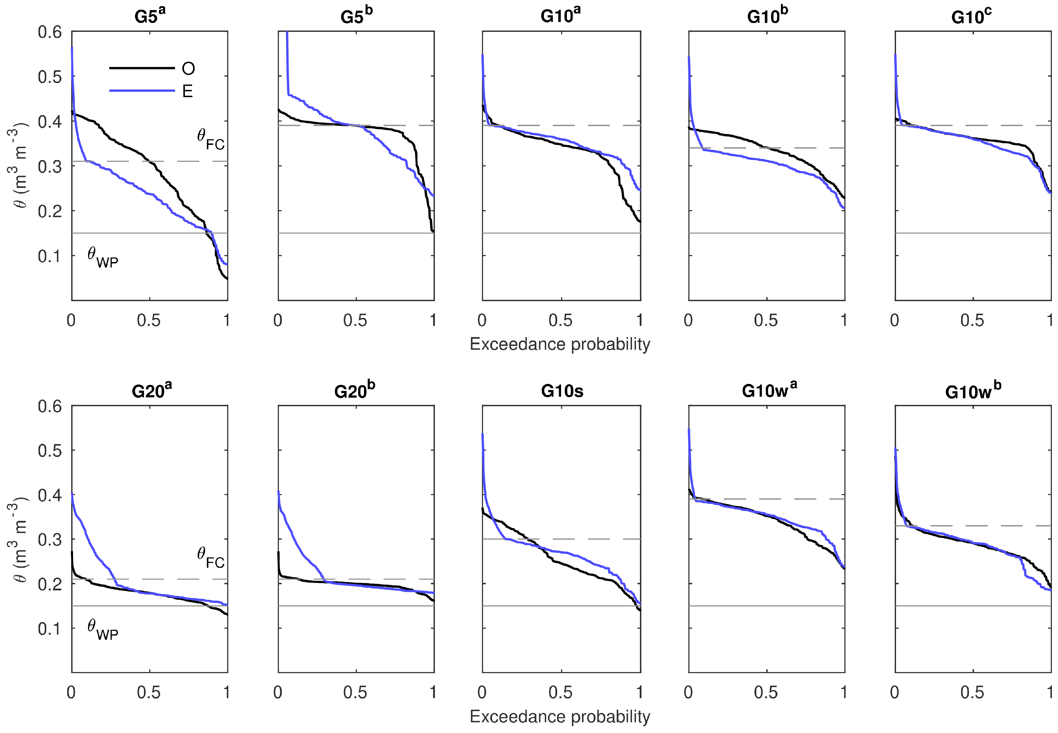
3.1.2. Validation Phase

Based on the estimated parameters for the substrate and the vegetation, the VWC of the substrate of each specimen was simulated by the calibrated model for the validation period. Ten rainfall events occurred during this period, accumulating 177.6 mm (Figure 4 upper). The three largest events took place on 11 July (31 mm), 5 August (100.6 mm) and 7 September (15.4 mm). The parameters used in this simulation are the same as in Table 2 and Table 3, with the exception of the initial substrate moisture ${\theta }_i$ which was taken as the first record of the data set of this new test period (values are given in

Table 5. MCE, MAE, mean (μ) and standard deviation (σ) from observed (O) and estimated (E) volumetric water content (VWC) during the rainy season 2015.

Group	ID	${\mathit{\theta }}_{\mathit{i}}$ (m3 m−3)	MCE	MAE	$\mathit{\mu }$ (VWC)		$\mathit{\sigma }$ (VWC)
					O	E	O	E
G5	G5a	0.405	0.25	0.06	0.282	0.233	0.102	0.076
	G5b	0.403	−0.24	0.04	0.371	0.382	0.054	0.087
G10	G10a	0.383	0.48	0.02	0.334	0.351	0.058	0.039
	G10b	0.383	0.11	0.03	0.332	0.305	0.041	0.041
	G10c	0.395	0.59	0.01	0.357	0.352	0.034	0.040
G20	G20a	0.197	−0.96	0.03	0.178	0.211	0.022	0.053
	G20b	0.206	−2.50	0.03	0.198	0.218	0.012	0.050
G10s	G10s	0.350	0.55	0.02	0.256	0.267	0.058	0.053
G10w	G10wa	0.385	0.67	0.01	0.340	0.348	0.044	0.040
	G10wb	0.325	0.60	0.01	0.288	0.285	0.039	0.049

). Figure 4 shows the simulated (estimated) and measured (observed) substrate moisture curves during the test period, for each specimen. Furthermore, Table 5 shows the goodness-of-fit metrics. μ and σ from observed (O) and estimated (E) data are also presented.

The agreement between measurements and simulations results is less than that obtained for the calibration phase. The highest deviation occurs after the largest precipitation event, in early August. During this event, the soil moisture of the substrate is overestimated for all specimens. For specimens G20^a, G20^b, G5^b, the overestimation from the model is large enough to obtain negative MCE values, which implies that the predictive power of the model for these cases is less than that of the average of the observations. Nevertheless, the simulation curve joins the measurement in most cases in a short-time period after the precipitation event (specimens G20 take more time). In specimen G5^a the substrate moisture is systematically underestimated by the model. The best agreement is for the specimens of 10 cm depth (G10, G10s, G10w). The specimens G10w present a good fit, even just after the largest precipitation event, with MCE values higher than 0.6 and MAE values lower than the standard deviation. A possible reason for this is that these specimens do not have a drainage layer, which facilitated the calibration of the S parameter. Overall, the estimated results can be considered as good despite the differences observed in some cases because it should be kept in mind that the conditions of vegetation, drainage system and substrate could have varied since the beginning of the experiment and altered some substrate or vegetation parameters [13]. For example, the development of vegetation roots after one year could change the composition and properties of the root region, which can affect the predicted results of the model. Interestingly, vegetation developed the most during the validation period precisely in the 20 cm depth specimens, in which the model performs the worst. Moreover, the sponge-type drainage system of specimen G5^b also facilitated a vegetation development much stronger than that in specimen G5^a. These changes may have altered the root region particularly in these specimens in a way not captured by the model. Furthermore, because the same vegetation was used in all the specimens, it is not possible to come up with a comparison-based analysis to fully characterize the role of the vegetation and its dynamic on the overall performance of the roofs.

When comparing the moisture curves for all specimens, we can first highlight the impact of the substrate depth. Specimens G5^a and G10^a are equipped with the same drainage system (Sika^® Sarnavert Aquadrain) but have different substrate depths (5 cm <> 10 cm). Substrate moisture is less variable over time in specimen G10^a as compared to G5^a. The same observation can be made between the specimens G10s (10 cm) and G20^b (20 cm) equipped with the same drainage system (Delta^®-Floraxx). We can also highlight the impact of the drainage system by comparing the different specimens within a same group.

3.2. Performance Assessment

3.2.1. Irrigation Needs

From the knowledge of the substrate water content dynamics over time shown in the previous sections, the number of days for which irrigation is needed was determined for the rainy seasons 2014 and 2015, for all green roof specimens. Figure 5 and Figure 6 show the substrate water content duration (SWCD) curve of each specimen during the rainy seasons of 2014 and 2015, respectively. The SWCD curve allows us to characterize the overall dynamics of the substrate moisture and to detect the number of days in which a particular value is or is not exceeded [14]. In these figures, both observed (O) and estimated (E) results are drawn. In this case, the wilting point (${\theta }_{WP}$), a common value for all specimens (${\theta }_{WP}$ = 0.15, see Table 2), is used to compare the VWC behavior. The content ${\theta }_{WP}$is a critical value that compromises the plant health, as at a value less than ${\theta }_{WP}$, the plant will wither permanently [26]. Thus, under this value, irrigation should be essential.

Theoretically, the amount of water available for the plant is the gap between ${\theta }_{FC}$ and ${\theta }_{WP}$ [26]. During the preliminary laboratory experiments, it was concluded that the amount of water delivered by precipitation during the study period was sufficient for all specimens. This was corroborated by the frequent visual inspection of the vegetation condition during the testing period. In fact, some plant growth was observed, demonstrating that this type of vegetation requires little water to survive [5,16,33]. This observation suggests that the survival line of the plant could be under the ${\theta }_{WP}$. However, for simplicity, we choose to maintain ${\theta }_{WP}$ as the limit value.

Figure 5 shows a close agreement between the observed and simulated SWCD curves, reflecting the ability of the model to reproduce the soil moisture dynamics during the calibration period. Even if some deviation was previously observed between the individual values of the simulated and the measured water content during the validation period (Figure 4), Figure 6 shows similar values of simulated and observed soil moisture corresponding to high values of exceedance probability (between 0.8 and 1) for all the specimens. The good agreement for these values of exceedance probability allows an accurate estimation of the irrigation needs. For example, in specimen G5^a, both measured and modeled data indicate that this specimen would require irrigation about 10% of the time under evaluation (i.e., 9–10 days for the study period). Also, modeled and measured SWCD curves of G10, G10s and G10w have similar behavior. In the case of G20, the two curves are in good agreement for probability of exceedance larger than 0.4; the higher deviation below this probability value is explained by the high discrepancy after the great precipitation event during August 2015 as observed in Figure 4.

The simulations with the model show that specimens of 10 cm depth are the best in terms of the relationship between amount of irrigation and plant survival, with no or little need of irrigation for the considered period. This is explained by a greater amount of available water for the plant due to a deeper substrate compared to the 5 cm specimens, and to a higher value of the field capacity (${\theta }_{FC}$) compared to the 20 cm specimens. Indeed, the 20 cm specimens in this study are characterized by a small ${\theta }_{FC}$, close to the wilting point${\theta }_{WP}$. On the other hand, the 5 cm specimen modeled without the drainage layer (G5^a), reached the lowest substrate moisture values, even less than the wilting point. This in turns explains the irrigation need previously mentioned. This result is expected because the water retention capacity typically decreases for thinner substrate depths. In fact, substrate depths of less than 7 cm are not recommended for Sedum as the water holding capacity is very low [34].

3.2.2. Water Runoff

The runoff performance was assessed by simulation, using the validated model explained in the previous sections. By simulating all hydrological processes in detailed according to Figure 2, the model is able to produce surface and subsurface hydrographs. No comparison with measurement data was made, because the runoff was not measured. The water runoff from green roofs can be superficial and/or subsuperficial depending on the roof design and magnitude of precipitation event [16]. In both cases, water flows outside the building through guttering. In the particular case of the green roof specimens tested in the LIVE, all specimens are characterized by a superficial storage capacity of at least 10 cm. Furthermore, the substrate used has a high hydraulic conductivity, which infiltrates all water that precipitates in the area. As a consequence, the water flow produced by all specimens is only composed of percolated fluxes so it can be characterized as subsuperficial runoff.

Table 6. Hydrological information of each precipitation event during the 2014 and 2015 winter seasons.

N°		1	2	3	4	5	6	7	8	9	10	11	12	13	14	15	16	17	18	19	20	Total
Initial Date (Day-Month-Year)		02-07-2014	14-07-2014	03-08-2014	06-08-2014	23-08-2014	30-08-2014	01-09-2014	05-09-2014	13-09-2014	22-09-2014	05-07-2015	11-07-2015	30-07-2015	02-08-2015	05-08-2015	09-08-2015	12-08-2015	06-09-2015	07-09-2015	09-09-2015
Precipitation (mm)		7.0	35.6	2.2	15.6	35.2	7.0	7.2	11.8	13.8	1.6	1.2	31.0	6.0	1.6	100.6	8.2	10.8	1.0	15.4	1.8	314.6
Duration (days)		0.2	0.3	0.1	0.2	1.6	0.1	0.3	0.3	0.4	0.6	0.1	2.0	0.4	0.1	3.1	0.4	0.2	0.2	1.0	0.1	11.7
Mean intensity (mm h−1)		1.9	4.5	0.8	2.8	0.9	3.8	1.0	2.0	1.6	0.1	1.3	0.7	0.6	0.5	1.4	0.9	2.2	0.2	0.7	1.0	1.1
Max intensity (mm h−1)		7.2	16.8	4.8	7.2	14.4	9.6	7.2	14.4	7.2	2.4	2.4	7.2	7.2	2.4	14.4	9.6	12.0	2.4	4.8	4.8	16.8
Dry days		19.6	12.2	19.4	2.8	17.1	5.1	2.0	3.5	8.1	8.1	64.4	5.4	17.8	1.9	3.1	1.1	2.3	24.6	0.7	1.5	220.7
${\theta }_i$ (m3 m−3)	G5a	0.21	0.17	0.17	0.17	0.10	0.23	0.28	0.29	0.19	0.17	0.20	0.18	0.25	0.33	0.31	0.41	0.41	0.05	0.05	0.25	--
	G5b	0.36	0.36	0.35	0.35	0.31	0.36	0.38	0.38	0.36	0.35	0.38	0.37	0.38	0.39	0.39	0.41	0.41	0.16	0.15	0.35	--
	G10a	0.37	0.36	0.36	0.36	0.33	0.37	0.38	0.38	0.36	0.36	0.31	0.28	0.32	0.34	0.33	0.39	0.39	0.18	0.18	0.34	--
	G10b	0.33	0.32	0.31	0.31	0.26	0.31	0.33	0.33	0.29	0.28	0.33	0.31	0.30	0.33	0.33	0.37	0.38	0.23	0.23	0.30	--
	G10c	0.37	0.36	0.36	0.36	0.35	0.37	0.38	0.38	0.36	0.35	0.35	0.35	0.35	0.37	0.36	0.39	0.39	0.24	0.24	0.35	--
	G20a	0.17	0.16	0.16	0.16	0.14	0.18	0.19	0.19	0.16	0.15	0.17	0.16	0.17	0.18	0.18	0.21	0.21	0.13	0.13	0.16	--
	G20b	0.22	0.22	0.20	0.20	0.19	0.21	0.21	0.21	0.20	0.19	0.20	0.19	0.19	0.20	0.20	0.21	0.21	0.16	0.16	0.19	--
	G10s	0.25	0.23	0.25	0.26	0.23	0.28	0.29	0.29	0.24	0.21	0.22	0.21	0.22	0.24	0.23	0.34	0.35	0.14	0.14	0.21	--
	G10wa	0.37	0.36	0.36	0.36	0.31	0.37	0.37	0.38	0.35	0.33	0.29	0.28	0.31	0.35	0.35	0.39	0.39	0.24	0.23	0.33	--
	G10wb	0.29	0.28	0.28	0.28	0.22	0.29	0.30	0.30	0.26	0.24	0.27	0.26	0.27	0.29	0.29	0.34	0.34	0.20	0.19	0.26	--
$C$	G5a	0.00	0.65	0.00	0.24	0.59	0.00	0.03	0.46	0.17	0.00	0.00	0.50	0.00	0.00	0.87	1.75	0.91	0.00	0.00	0.10	0.58
	G5b	0.00	0.44	0.00	0.00	0.25	0.00	0.00	0.00	0.00	0.00	0.00	0.10	0.00	0.00	0.48	3.84	0.97	0.00	0.00	0.00	0.38
	G10a	0.00	0.66	0.00	0.21	0.55	0.00	0.09	0.39	0.21	0.00	0.00	0.43	0.00	0.00	0.87	1.75	0.95	0.00	0.00	0.00	0.57
	G10b	0.13	0.60	0.00	0.15	0.49	0.00	0.00	0.29	0.14	0.00	0.00	0.39	0.00	0.00	0.84	1.80	0.94	0.00	0.00	0.00	0.54
	G10c	0.02	0.70	0.00	0.25	0.57	0.00	0.17	0.44	0.25	0.00	0.00	0.48	0.00	0.00	0.89	1.75	0.95	0.00	0.00	0.00	0.60
	G20a	0.05	0.05	0.08	0.05	0.02	0.03	0.05	0.05	0.03	0.22	0.00	0.00	0.00	0.00	0.20	1.70	1.69	0.00	0.00	0.00	0.18
	G20b	0.14	0.13	0.11	0.04	0.03	0.04	0.06	0.05	0.00	0.00	0.00	0.00	0.00	0.00	0.23	1.36	1.65	0.00	0.00	0.00	0.19
	G10s	0.00	0.47	0.00	0.06	0.40	0.00	0.00	0.21	0.07	0.00	0.00	0.31	0.00	0.00	0.78	2.13	0.95	0.00	0.00	0.00	0.48
	G10wa	0.04	0.68	0.00	0.23	0.56	0.00	0.13	0.41	0.23	0.00	0.00	0.47	0.00	0.00	0.88	1.76	0.95	0.00	0.00	0.00	0.59
	G10wb	0.00	0.19	0.00	0.00	0.06	0.00	0.00	0.00	0.00	0.00	0.00	0.03	0.00	0.00	0.61	1.74	0.88	0.00	0.00	0.00	0.30

shows recorded information for each precipitation event during rainy seasons of 2014 and 2015 (initial date, precipitation depth, duration, mean and max intensity, dry days before event and initial substrate moisture). Also, the runoff coefficient (C), which is the ratio between modeled percolated flows and precipitation, is presented. The last column of Table 6 shows the C_total, which was calculated from the total sum of percolation and precipitation for all studied events.

There is a clear relationship between the green roof capacity to control runoff and the depth of its substrate. The runoff coefficient C_total for the 20 cm depth specimens (G20, C_total = 0.18 and 0.19) is lower than that of the 5 or 10 cm specimens, retaining more water in its substrate. The same conclusion can be drawn when looking at all individual events with a significant precipitation larger than 30 mm (i.e., events N° 2, 5, 12 and 15). For those events, C_G20 reaches the lowest values. Refs. [13,16] came to similar conclusions. Secondly, the runoff coefficient is directly proportional to the duration and the magnitude of precipitation events [16]. On the one hand, when events are small, runoff is null in the vast majority of cases. For instance, the magnitude of the events N° 3, 10, 11, 14, 18, and 20 does not exceed 3 mm so no outflow is generated. That was also reported in [16] where the authors did not observe outflow for 5 and 10 cm specimens up to 4 mm of rainfall. On the other hand, when rainfall is higher, the runoff coefficients are higher too. The coefficient is even close to 1 for some specimens for the event N° 15 with the highest rainfall. While C is generally <1, this value could be greater than 1 when it is calculated for an individual event, because the runoff could include water stored during a previous event. This occurs, for example, in event N° 16 which is separated by only 1.1 days from event N° 15, the largest precipitation event during the study period. The proximity between the two events implies an impact on the initial substrate moisture, which is another influential factor in the runoff control [16]. In fact, event N° 19 is characterized by median magnitude and median intensity (15.4 mm during 1 day) which does not generate outflow. This occurs because in this event, the initial substrate moisture is much less than the field capacity, even reaching the wilting point.

Finally, it is important to remember that all values of runoff coefficient were obtained from simulated data. According to [16], experimental values of runoff coefficient would be lower than those of Table 6 since the experiment is composed of other constructional elements which can retain additional water. As mentioned in Section 2.2.2, in the context of this study, the drainage layer was not modeled except for specimen G5^b that was equipped with a very absorbing drainage system. In the last column of Table 6, we can indeed see that the mean coefficient C for specimen G5^b is lower than for the other 5 or 10 cm specimens.

4. Conclusions

This study showed the full potential of the hydrologic model IHMORS to correctly evaluate the hydrological behavior of a wide variety of green roofs and estimate the potential irrigation needs and runoff control performance. This was made possible by an accurate modeling of all surface and subsurface processes occurring in green roofs. Furthermore, the model continuously simulates the performance of green roofs over a full season and not just for specific events. The model was validated against a full set of green roofs with different constructive characteristics for the specific semiarid climate encountered in the central part of Chile. Our main conclusions are the following:

• IHMORS is capable of characterizing many different variables of green roofs, such as the geometry, vegetation, substrate type and depth, and drainage system. In particular IHMORS was successfully calibrated to 10 different specimens (and two more replicas of one of them).
• The calibrated model predicted the volumetric water content (VWC) dynamics of the 10 cm depth specimens quite well, especially those with no drainage layer. The estimated VWC was less accurate for the 5 and 20 cm specimens. The larger errors obtained for those specimens with stronger vegetation development suggest the necessity for a better understanding of the effects of the vegetation changes on the substrate, and the definition of modelling strategies to represent such changes.
• By means of the soil water content duration curve, the model can be used to estimate the number of days in which irrigation may be needed to preserve a target soil moisture. Such application shows how the 5 cm depth specimen with no drainage layer reaches substrate moisture values lower than the wilting point. During these days (~10% of the study period) irrigations should be considered.
• The simulation of the runoff coefficients using the model yields very reasonable results. For all the rain events, the lowest runoff coefficient was simulated for the 20 cm specimens. Moreover, small events (<3 mm) did not produce outflow from any specimen. Finally, the simulated runoff coefficients were directly proportional to the duration and the magnitude of the rainfall events.

As further research, it would be interesting to see if a finer modeling using IHMORS (i.e., the modeling of the drainage system for all green roof specimens and the subdivision of the substrate layer in several slices) could deliver more accurate results. Moreover, the model can be used in roof design by choosing the most appropriate vegetation, substrate and drainage system in order to reduce the water needs while preserving enough soil moisture for plant survival. Finally, IHMORS could be coupled to a thermal model to optimize both the hydrological and the energy performance of green roofs by reducing water and energy needs.

References

1. Berndtsson, J.C. Green roof performance towards management of runoff water quantity and quality: A review. Ecol. Eng. 2010, 36, 351–360. [Google Scholar] [CrossRef]
2. Novotny, V.; Ahern, J.; Brown, P. Water Centric Sustainable Communities: Planning, Retrofitting, and Building the Next Urban Environment; John Wiley & Sons: Hoboken, NJ, USA, 2010; ISBN 978-0-470-47608-6. [Google Scholar]
3. Rossmiller, R.L. Stormwater Design for Sustainable Development; Mc Graw Hill Education: Columbus, OH, USA, 2014; ISBN 978-0071816526. [Google Scholar]
4. Liu, K.; Baskaran, B. Thermal performance of green roofs through field evaluation. In Proceedings of the First North American Green Roof Infrastructure Conference, Awards and Trade Show, Chicago, IL, USA, 29–30 May 2003; pp. 1–10. [Google Scholar]
5. Reyes, R.; Bustamante, W.; Gironás, J.; Pastén, P.A.; Rojas, V.; Suárez, F.; Vera, S.; Victorero, F.; Bonilla, C.A. Effect of substrate depth and roof layers on green roof temperature and water requirements in a semi-arid climate. Ecol. Eng. 2016, 97, 624–632. [Google Scholar] [CrossRef]
6. Van Mechelen, C.; Dutoit, T.; Hermy, M. Adapting green roof irrigation practices for a sustainable future: A review. Sustain. Cities Soc. 2015, 19, 74–90. [Google Scholar] [CrossRef]
7. Nektarios, P.A.; Amountzias, I.; Kokkinou, I.; Ntoulas, N. Green roof substrate type and depth affect the growth of the native species Dianthus fruticosus under reduced irrigation regimens. HortScience 2011, 46, 1208–1216. [Google Scholar]
8. Issa, R.J.; Leitch, K.; Chang, B. Experimental heat transfer study on green roofs in a semiarid climate during summer. J. Constr. Eng. 2015, 2015, 960538. [Google Scholar] [CrossRef]
9. Vera, S.; Bonilla, C.; Victorero, F.; Gironás, J.; Bustamante, W.; Rojas, M.V. Soluciones Integrales de Cubiertas Vegetales Sustentables para Edificios Comerciales-Industriales en Climas Semiaridos de Chile; Informe Técnico Final, Proyecto INNOVACHILE 12IDL2-13630; Departamento de Ingeniería y Gestión de la Construcción, Escuela de Ingeniería, Pontificia Universidad Católica de Chile: Santiago, Chile, 2014. [Google Scholar]
10. Dvorak, B.; Volder, A. Plant establishment on unirrigated green roof specimens in a subtropical climate. AoB Plants 2013, 5, pls049. [Google Scholar] [CrossRef]
11. Sample, D.J.; Heaney, J.P. Integrated management of irrigation and urban stormwater infiltration. J. Water Resour. Plan. Manag. 2006, 132, 362–373. [Google Scholar] [CrossRef]
12. Houdeshel, C.D.; Hultine, K.R.; Johnson, N.C.; Pomeroy, C.A. Evaluation of three vegetation treatments in bioretention gardens in a semi-arid climate. Landsc. Urban Plan. 2015, 135, 62–72. [Google Scholar] [CrossRef]
13. Berretta, C.; Poë, S.; Stovin, V. Moisture content behaviour in extensive green roofs during dry periods: The influence of vegetation and substrate characteristics. J. Hydrol. 2014, 511, 374–386. [Google Scholar] [CrossRef]
14. Herrera, J.; Bonilla, C.A.; Castro, L.; Vera, S.; Reyes, R.; Gironás, J. A model for simulating the performance and irrigation of green stormwater facilities at residential scales in semiarid and Mediterranean regions. Environ. Model. Softw. 2017, 95, 246–257. [Google Scholar] [CrossRef]
15. Li, Y.; Babcock, R.W., Jr. Green roof hydrologic performance and modeling: A review. Water Sci. Technol. 2014, 69, 727–738. [Google Scholar] [CrossRef] [PubMed]
16. Feitosa, R.C.; Wilkinson, S. Modelling green roof stormwater response for different substrate depths. Landsc. Urban Plan. 2016, 153, 170–179. [Google Scholar] [CrossRef]
17. Hilten, R.N.; Lawrence, T.M.; Tollner, E.W. Modeling stormwater runoff from green roofs with HYDRUS-1D. J. Hydrol. 2008, 358, 288–293. [Google Scholar] [CrossRef]
18. Hakimdavar, R.; Culligan, P.J.; Finazzi, M.; Barontini, S.; Ranzi, R. Scale dynamics of extensive green roofs: Quantifying the effect of drainage area and rainfall characteristics on observed and modeled green roof hydrologic performance. Ecol. Eng. 2014, 73, 494–508. [Google Scholar] [CrossRef]
19. Qin, H.; Peng, Y.; Tang, Q.; Yu, S. A HYDRUS model for irrigation management of green roofs with a water storage layer. Ecol. Eng. 2016, 95, 399–408. [Google Scholar] [CrossRef]
20. Li, Y.; Babcock, R.W., Jr. Modeling Hydrologic Performance of a Green Roof System with HYDRUS-2D. J. Environ. Eng. 2015, 141, 04015036. [Google Scholar] [CrossRef]
21. Palla, A.; Gnecco, I.; Lanza, L.G. Compared performance of a conceptual and a mechanistic hydrologic models of a green roof. Hydrol. Process. 2012, 26, 73–84. [Google Scholar] [CrossRef]
22. Peng, L.L.; Jim, C.Y. Seasonal and diurnal thermal performance of a subtropical extensive green roof: The impacts of background weather parameters. Sustainability 2015, 7, 11098–11113. [Google Scholar] [CrossRef] [Green Version]
23. Locatelli, L.; Mark, O.; Mikkelsen, P.S.; Arnbjerg-Nielsen, K.; Bergen Jensen, M.; Binning, P.J. Modelling of green roof hydrological performance for urban drainage applications. J. Hydrol. 2014, 519, 3237–3248. [Google Scholar] [CrossRef]
24. Peel, M.C.; Finlayson, B.L.; McMahon, T.A. Updated world map of the Köppen-Geiger climate classification. Hydrol. Earth Syst. Sci. 2007, 11, 1633–1644. [Google Scholar] [CrossRef]
25. Dirección General de Aeronáutica Civil (DGAC). Dirección Meteorológica de Chile. Available online: http://www.meteochile.cl (accessed on 23 July 2015).
26. Sandoval, V.; Suárez, F.; Vera, S.; Pinto, C.; Victorero, F.; Bonilla, C.; Gironás, J.; Bustamante, W.; Rojas, V.; Pastén, P. Impact of the Properties of a Green Roof Substrate on its Hydraulic and Thermal Behavior. Energy Procedia 2015, 78, 1177–1182. [Google Scholar] [CrossRef]
27. Vera, S.; Gironás, J.; Victorero, F.; Schöll, M.; Bonilla, C.; Bustamante, W.; Rojas, M.V. Informe Catastro; Proyecto INNOVACHILE 12IDL2-13630; Departamento de Ingeniería y Gestión de la Construcción, Escuela de Ingeniería, Pontificia Universidad Católica de Chile: Santiago, Chile, 2014. [Google Scholar]
28. Allen, R.G.; Pereira, L.S.; Raes, D.; Smith, M. Crop Evapotranspiration: Guidelines for Computing Crop Water Requirements; FAO Irrigation and Drainage Paper: Rome, Italy, 1998. [Google Scholar]
29. Sherrard, J.A.; Jacobs, J.M. Vegetated roof water-balance model: Experimental and model results. J. Hydrol. Eng. 2005, 17, 858–868. [Google Scholar] [CrossRef]
30. Bennett, N.D.; Croke, G.F.W.; Guariso, G.; Guillaume, J.H.A.; Hamilton, S.H.; Jakeman, A.J.; Marsili-Libelli, S.; Newham, L.T.H.; Norton, J.P.; Perrin, C.; et al. Characterising performance of environmental models. Environ. Model. Softw. 2013, 40, 1–20. [Google Scholar] [CrossRef]
31. Legates, D.R.; McCabe, G.J. Evaluating the use of “goodness-of-fit” measures in hydrologic and hydroclimatic model validation. Water Resour. Res. 1999, 35, 233–241. [Google Scholar] [CrossRef]
32. Savabi, M.R.; Williams, J.R. Evaporation and Environment; WEPP Model Documentation; USDA-ARS National Substrate Erosion Research Laboratory Publication: Washington, DC, USA, 1995.
33. Schroll, E.; Lambrinos, J.G.; Sandrock, D. An evaluation of plant selections and irrigation requirements for extensive green roofs in the Pacific northwestern United States. HortTechnology 2011, 1, 314–322. [Google Scholar]
34. Getter, K.L.; Rowe, D.B. Substrate depth influences sedum plant community on a green roof. HortScience 2009, 44, 401–407. [Google Scholar]
Figure 1. Photo of green roof specimens tested in the LIVE.
Water 10 00198 g001
Figure 2. Conceptual representation of the physical processes simulated in IHMORS (extracted from [14]).
Water 10 00198 g002
Figure 3. Observed (O) (black lines) and estimated (E) (blue lines) substrate moisture during calibration process (rainy season 2014). A precipitation hyetograph is also presented.
Water 10 00198 g003
Figure 4. Observed (O) (black lines) and estimated (E) (blue lines) substrate moisture during the rainy season 2015. The precipitation hyetograph is also presented.
Water 10 00198 g004
Figure 5. Observed (O) (black lines) and estimated (E) (blue lines) soil water content duration curve for each specimen during the rainy season 2014.
Water 10 00198 g005
Figure 6. Observed (O) (black lines) and estimated (E) (blue lines) soil water content duration curve for each specimen during the rainy season 2015.
Water 10 00198 g006