Ecohydrologic Connections in Semiarid Watershed Systems of Central Oregon USA
by
 ,
,
Carlos G. Ochoa
1,* ,
,
Phil Caruso
2,
Grace Ray
3,
Tim Deboodt
4,
W. Todd Jarvis
5 and
Steven J. Guldan
6 1
Department of Animal and Rangeland Sciences, Oregon State University, Corvallis, OR 97331, USA
2
Water Resources Graduate Program, Oregon State University, Corvallis, OR 97331, USA
3
Natural Resources Division, Turner Enterprises, Inc., Bozeman, MT 59718, USA
4
OSU Extension Service-Crook County, Oregon State University, Prineville, OR 97754, USA
5
Institute for Water and Watersheds, Oregon State University, Corvallis, OR 97331, USA
6
Sustainable Agriculture Science Center, New Mexico State University, Alcalde, NM 87511, USA
*
Author to whom correspondence should be addressed.
Water 2018, 10(2), 181; https://doi.org/10.3390/w10020181
Submission received: 26 December 2017
/
Revised: 31 January 2018
/
Accepted: 5 February 2018
/
Published: 9 February 2018
Abstract
:An improved understanding of ecohydrologic connections is critical for improving land management decisions in water-scarce regions of the western United States. For this study, conducted in a semiarid (358 mm) rangeland location in central Oregon, we evaluated precipitation-interception-soil moisture dynamics at the plot scale and characterized surface water and groundwater relations across the landscape including areas with and without western juniper (Juniperus occidentalis). Results from this study show that juniper woodlands intercepted up to 46% of total precipitation, altering soil moisture distribution under the canopy and in the interspace. Results indicate that precipitation reaching the ground can rapidly percolate through the soil profile and into the shallow aquifer, and that strong hydrologic connections between surface and groundwater components exist during winter precipitation and snowmelt runoff seasons. Greater streamflow and springflow rates were observed in the treated watershed when compared to the untreated. Streamflow rates up to 1020 L min−1 and springflow rates peaking 190 L min−1 were observed in the watershed where juniper was removed 13 years ago. In the untreated watershed, streamflow rates peaked at 687 L min−1 and springflow rates peaked at 110 L min−1. Results contribute to improved natural resource management through a better understanding of the biophysical connections occurring in rangeland ecosystems and the role that woody vegetation encroachment may have on altering the hydrology of the site.
1. Introduction
In many dryland ecosystems worldwide, woody vegetation has expanded rapidly while open grassland vegetation has declined significantly over the last century or more [1,2,3]. This progressive shift from grasses to woody species has resulted in larger bare soil areas and decreased vegetation diversity [4] promoting increased runoff velocities and more soil erosion [5]. According to the Intergovernmental Panel on Climate Change, expected changes in climate will worsen the loss of biodiversity and decrease water availability and quality in many of these arid and semiarid regions around the globe [6]. Among the array of woody species that have significantly expanded across the western United States, juniper (Juniperus spp.) now covers nearly 40 million hectares [7]. Commonly attributed causes of juniper expansion are a mix of biophysical and anthropogenic factors including overgrazing, increases in CO2, and fire suppression [8]. An estimated tenfold increase in juniper cover has occurred in the past 130 years [9]. In Oregon, western juniper (Juniperus occidentalis) is the dominant juniper species and has increased from 420,000 acres in 1936 [10] to more than 3.5 million acres [11]. Western juniper is commonly found in areas with annual precipitation ranging between 230 and 355 mm [12], at elevations between 1370 and 2440 m [13].
Striking landscape changes attributed to high levels of encroachment into sagebrush-steppe [9,14] and grassland ecosystems [15,16] have raised considerable concerns about the negative impacts of juniper expansion on multiple ecosystem functions and services provided. Juniper encroachment into these rangeland ecosystems can limit the growth of shrubs, grasses, and forbs, by outcompeting them for light, soil moisture, and soil nutrients [17,18,19]; reduce biodiversity [20,21,22]; alter soil nutrient cycling [23]; and modify hydrologic processes such as evapotranspiration and soil moisture [24,25,26]. Studies conducted at relatively small scales have shown that the reduction of juniper stands through fire, herbicide, or mechanical methods have resulted in significant improvements to the treated areas. For example, juniper removal has resulted in reduction of runoff and soil erosion rates [27], higher infiltration rates [28], increases in herbaceous cover, stabilization of soils, and supporting of surface fire [29]. The effects of juniper reduction in water yields such as streamflow and groundwater recharge are less evident. Several authors have stated that marginal to no response in streamflow should be expected from juniper removal mainly because of the low precipitation and the high evaporation losses associated with juniper landscapes [30,31,32]. Hibbert [30] concluded that some potential for increasing water yields through vegetative manipulation exists in cool climate rangeland ecosystems where annual precipitation that concentrates in the winter is >400 mm; for warm climate landscapes, the threshold is >450 mm.
The number of studies addressing juniper reduction effects on water yield in cool climates is limited. It is increasingly recognized that juniper expansion effects on hydrologic processes such as groundwater recharge must be better understood and that a more integrated understanding of juniper landscape-scale processes is needed. As stated by Miller [8], no watershed scale studies exist that document western juniper effects on groundwater flow, and only anecdotal information is available to document the drying or regaining of stream and spring flows in response to juniper presence or removal. Comprehensive resource management requires evaluation and integration of surface water and groundwater components [33,34]. Surface water and groundwater cannot be seen as two isolated entities, there are multiple interactions that occur throughout the landscape between these two different components [35]. Surface water and groundwater connections can determine multiple biophysical relationships that are critical for the productivity of a given site. Hydrologic connections between upland water sources, groundwater, and downstream valleys influence the amount of water available for many ecosystem functions. Several studies have reported the temporally variable hydrologic connectivity between uplands and valleys [36,37,38,39,40]. These transient hydrologic connections have been found to vary spatially and temporally and are most often present during wet periods, when there is an increased input in precipitation or irrigation. Studies have shown there are direct connections between vegetation, hydrology, and other physical attributes such as topography and geology [41,42,43,44]. Most studies related to hydrologic connectivity have been done in mesic forests. The ecohydrologic linkages between upland water sources and downstream valleys in arid and semiarid regions are less understood. More studies focused on hydrologic connectivity under different geomorphic and climatic conditions are needed to improve understanding of the biophysical mechanisms that influence these connections [38].
This study aimed to enhance base knowledge regarding ecohydrologic relationships occurring in a semiarid rangeland ecosystem site in central Oregon in the USA. Study objectives were to: (1) assess precipitation-interception-soil moisture dynamics at the plot scale in a juniper-dominated watershed; and (2) characterize surface water and groundwater relations across the landscape including areas with and without juniper.
2. Materials and Methods
2.1. Description of Study Area
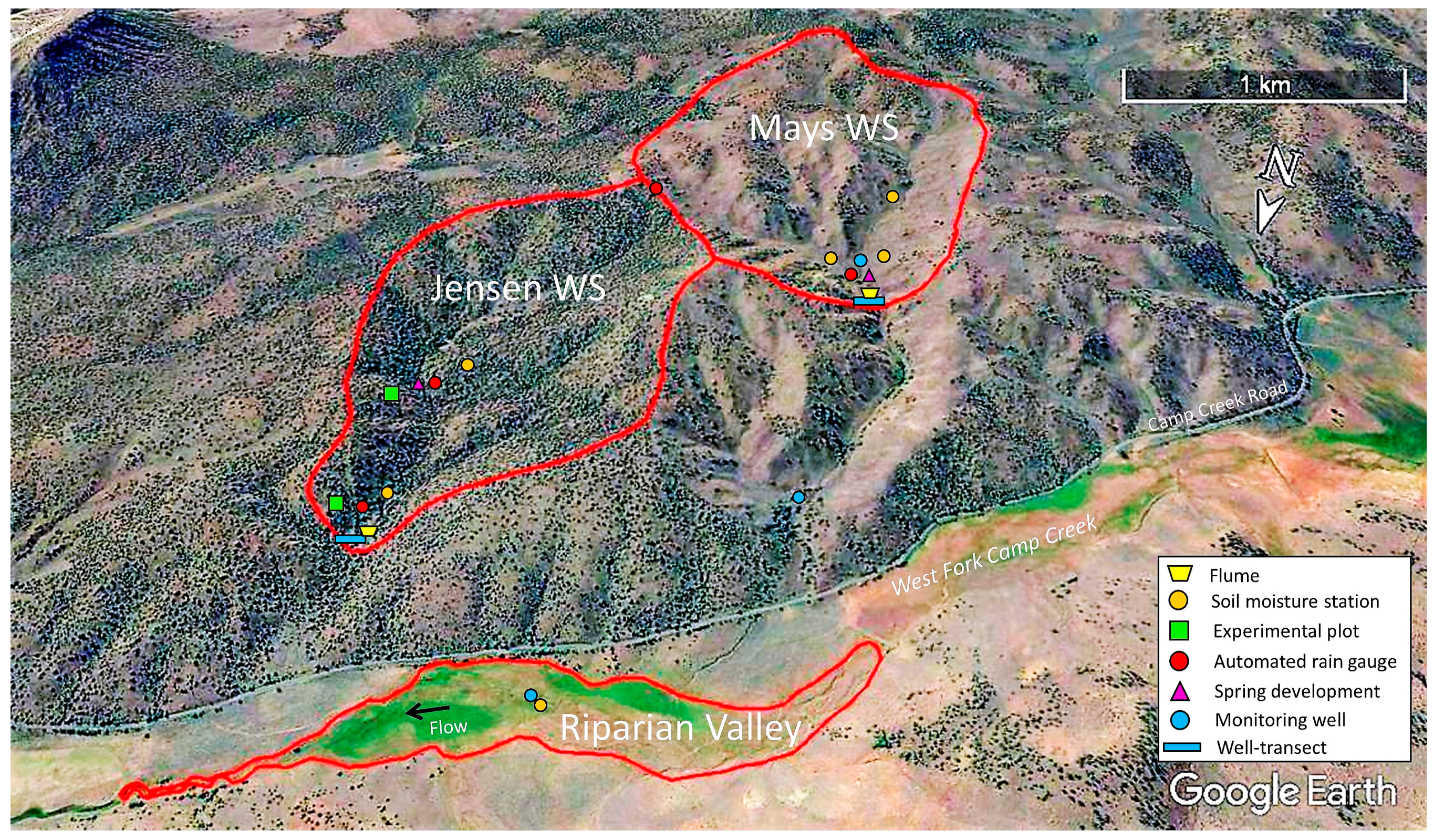
This study was conducted in the Camp Creek-Paired Watershed Study (CCPWS) site, 27 km northeast of Brothers, Oregon. The CCPWS site is a long-term collaborative research project located (43.96° Lat.; −120.34° Long.) in central Oregon [45]. The study area comprises one 116-ha watershed (Mays WS), one 96-ha watershed (Jensen WS), and a 20-ha section (Riparian Valley) of the West Fork Camp Creek. Elevation at the study site ranges from 1370 m in the Riparian Valley to 1524 m at the top of Mays WS. Dominant overstory vegetation in Jensen WS is western juniper. Dominant overstory vegetation in Mays WS is big sagebrush (Artemisia tridentata), this was after more than 90% of the juniper was removed. Juniper removal occurred during water year 2005–2006, it began in fall 2005 and ended in summer 2006 (hereafter the year of juniper removal will be designated 2006). Juniper removal consisted of cutting the trees with chainsaws at the base, removing boles, and scattering remaining limbs [45]. Prior to juniper removal, tree canopy cover was estimated to account for 27% of the total area in both watersheds. An intensive field study we conducted in 2015 to evaluate vegetation cover at the watershed scale shows Mays WS at <1% tree canopy cover and Jensen at 31% [46]. The slope in both watersheds ranges from an average 25% in west-facing slopes to 35% in north facing slopes [47]. The Riparian Valley site is largely a grassland (various spp.) area within two low dams and it is surrounded by sagebrush and western juniper vegetation. This valley section functioned as a sub-irrigated pasture for growing hay in the 1950s and 1960s and is now utilized as a summer grazing pasture. Similarly, both watersheds are also used for summer grazing purposes. Most precipitation in the area occurs as a mix of rain and snow during fall and winter, with sporadic rainfall events during spring and summer. Average annual precipitation recorded from 2009 to 2017 by onsite instrumentation was 358 mm. This is similar to the long-term (1961–2016) annual average precipitation (322 mm) reported by a nearby weather station (Barnes Station) located 10 km southeast of our study site [48].
In 2005, the two watersheds were instrumented to monitor multiple hydrologic variables including precipitation, soil moisture, runoff, and groundwater. Since October 2014, new instrumentation to measure selected variables (i.e., soil moisture, rainfall, and groundwater) has been added to expand the monitoring network in the watersheds and to include the Riparian Valley site (Figure 1).
Soils in the two watersheds are classified as Westbutte very stony loam, Madeline Loam, and Simas gravelly silt loam. Soils in the Riparian Valley site are classified as Bonnieview-Luckycreek complex [49]. Both Westbutte and Madeline series are moderately shallow to deep, well-drained soils and are formed of colluvium from weathered volcanic material such as basalt, andesite and tuff. Simas soils are very deep and well drained, formed of colluvium and loess from tuffaceaous sediments. Bonnieview series are very deep, moderately well drained and formed from residuum from weathered volcanic rock, and palesols. A series of streams that respond mostly to snowmelt runoff during the spring season are present in both watersheds. Occasional convective storms in the summer and fall also generate some ephemeral streamflow. The main stream draining out of Mays WS connects with the Riparian Valley downstream; however, the stream disappears in some areas at the bottom, only to resurface before reaching the Riparian Valley site. There is one relatively low flow spring in each of the two watersheds and in the Riparian Valley. The springs in the two watersheds were originally established for livestock watering decades prior to the study and were re-developed for the purpose of monitoring spring output in 2004 [45]. The study site overlies a shallow aquifer with depth to bedrock of approximately 9 m at the outlet of each watershed and in the Riparian Valley [45,46].
2.2. Field Data Collection
2.2.1. Soil Physical Properties
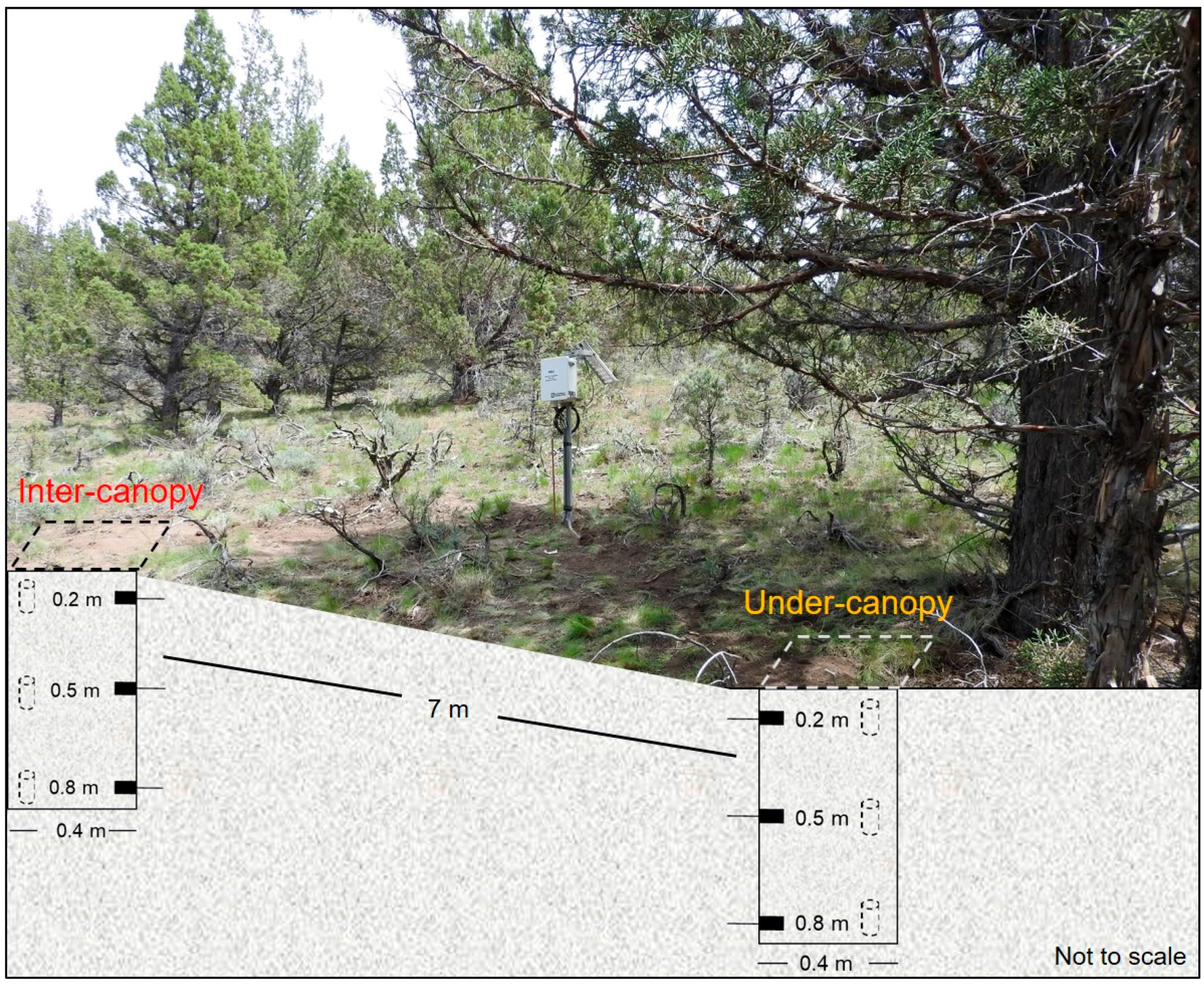
Soil samples for characterizing soil texture and bulk density were obtained during the most recent (2014–2015) soil moisture sensor installation in both watersheds and the Riparian Valley. At each sensor depth (Figure 2), three soil cores for bulk density and one loose soil sample for textural classification were collected. Soil texture was determined using the hydrometer method described by Gee and Bauder [50]. Soil bulk density was calculated using the protocol described by Blake and Hartge [51].
2.2.2. Precipitation Interception and Soil Moisture Content—Plot scale
The effects of tree-canopy cover on precipitation interception (I) and soil moisture content (θ) were evaluated at the plot scale in the Jensen WS (untreated). Two experimental plots of 2000 m2 each were installed to collect canopy cover, precipitation, and θ data (Figure 3). One of the plots was located at the valley bottom near the outlet of the watershed and the second plot was located 650 m upstream at a west-facing hillslope (~25% slope) near the stream (see Figure 1).
At each plot, twelve plastic rain-snow gauges (300-mL capacity) were installed on the ground. The gauges were installed at under-canopy (n = 4), inter-canopy (n = 4), and drip line (n = 4) locations. Rain gauges at under-canopy locations were installed at about half the distance from the trunk to the drip line. The gauges in the downstream plot were installed in October 2015 and the gauges in the upstream plot were installed in October 2016. The funnel top and inner tube of all gauges were removed during the winter season to capture snow precipitation. Snow and ice that formed in some of the gauges during the winter were melted to obtain precipitation water equivalent.
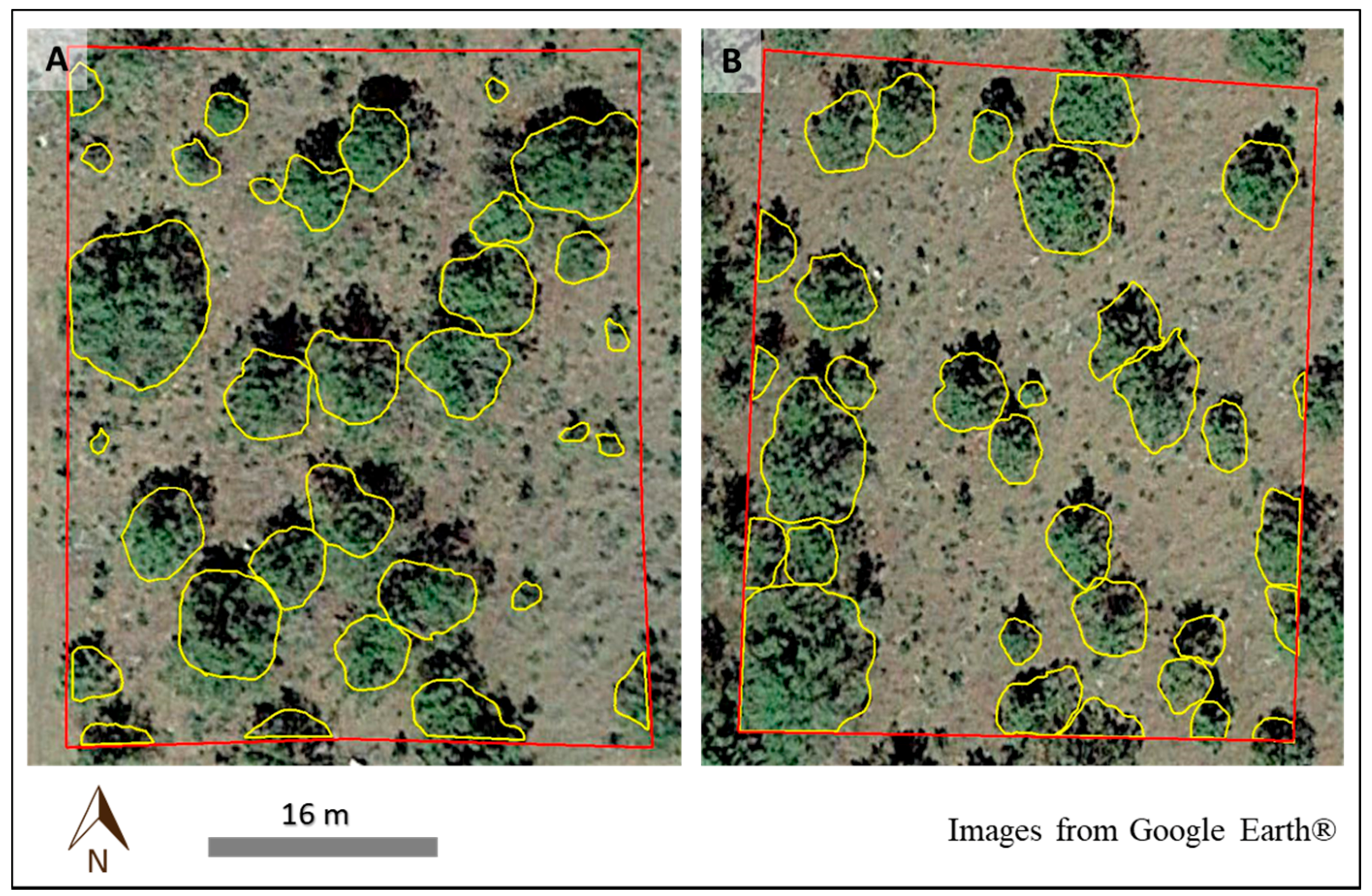
Tree canopy cover above each rain-snow gauge was estimated using a spherical crown densiometer (model A) using methodology adapted from Strickler [52]. Canopy cover at the entire 2000-m2 plot scale was calculated based on individual tree canopy area estimates in each plot. Canopy cover for each tree was delineated and area calculated using the polygon features in Google Earth®. In cases where tree canopy extended past plot boundaries we only accounted for the portion within the area of interest. The sum of all tree canopy areas was divided by the total plot area to determine plot scale canopy cover.
Precipitation interception was based on the amount of rain or snow reaching each rain-snow gauge. For each gauge location, I was calculated by subtracting the total amount of precipitation (P) collected in that particular gauge from the maximum amount of P recorded at the corresponding plot. The I values obtained for each rain gauge location were used to estimate average under-canopy (IUC), drip line (IDL), inter-canopy (IIC), and average I in each plot. We used the following equation to estimate average I in each plot.
where:
- I = Average precipitation interception in each plot;
- IUC = Precipitation interception at under-canopy locations;
- IDL = Precipitation interception at drip line locations;
- IIC = Precipitation interception at inter-canopy locations;
- n = number of rain gauges in each plot.
At each plot, a monitoring station with two vertical networks of three soil sensors each was installed to collect hourly θ data, one network was placed in the under-canopy location and one in the inter-canopy location. The under-canopy θ sensors were located 1 m north of the tree in the downstream plot and 1 m northwest of the tree in the upstream plot. The inter-canopy θ sensors were located 7 m north of the under-canopy θ sensors in both the downstream and the upstream plot. The θ sensors in each network were installed at 0.2, 0.5, and 0.8 m soil depth. For the upland plot, we used model CS650 sensors (Campbell Scientific, Inc., Logan, UT, USA). For the downstream plot, we used HydraProbe sensors (Stevens Water Monitoring Systems, Inc., Portland, OR, USA). Prior to field installation, all sensors were tested in the lab under air, water, and dry sand conditions. All sensors were within factory accuracy specifications. Sensors were not calibrated for site-specific soil characteristics. A Kruskal-Wallis One Way Analysis of Variance (ANOVA) on Ranks test was conducted to assess θ variability between inter-canopy and under-canopy locations in each experimental plot. Daily-averaged θ values at each sensor depth were used in this analysis. SigmaPlot® version 13.0 (Systat Software, Inc., San Jose, CA, USA) was used for all statistical analyses.
2.2.3. Surface Water and Groundwater Relations—Watershed Scale
Surface water and groundwater relationships among different components (i.e., precipitation, soil moisture, streamflow, springflow, and groundwater) were evaluated at the larger watershed scale. Most instrumentation mentioned in this section has been described in detail by Deboodt [45] and Ray [46]. Here we provide a brief description for convenience. Rainfall data were obtained using automated tipping-bucket rain gauges (Model RW100, Automata, Inc., Nevada City, CA, USA) distributed throughout the study site. Snowpack depth was measured using ultrasonic snow-depth recording sensors (Model TS-15S, Automata, Inc., Nevada City, CA, USA) located near the outlet in each watershed. Soil moisture data were obtained from sensors (Model AQUA-TEL-TDR, Automata, Inc., Nevada City, CA, USA) installed at 0.2, 0.5 and 0.8 m depth in monitoring stations installed in the interspace at upper and lower elevation areas in each watershed (see Figure 1). We averaged daily θ levels obtained during the three months (March through May) in the snowmelt runoff season where greater θ levels were observed every year (2014 through 2017). These three-month averaged θ values were used to compare inter-annual variability by sensor depth using a t-test analysis. Streamflow data were obtained using a Type-H flume [53] equipped with a water level logger installed in the main channel of each watershed. Manufacturer pre-calibrated equation and hourly-recorded water level data were used for estimating stream discharge. Springflow was measured at the outlet of a pipe installed as part of the spring development in each watershed. Except for the years 2014 and 2015, when no data were collected, springflow was measured from 2004 through 2017. Springflow data were collected at a minimum quarterly. During some years when more resources were available the measurement frequency increased to twice per month. For each springflow rate estimate we averaged (n = 5) the time to fill a 5-L container.
Automated records from 17 shallow (<10 m depth) monitoring wells were used to characterize groundwater level fluctuations. Data were obtained using previously installed transects of six wells, located perpendicular to the channel in each watershed [45], and a network of three wells installed in the Riparian Valley site in October 2014 [46]. The six-well transect in Mays WS spans 38 m across the watershed valley bottom and it is located at an elevation of 1438 m, in mostly fractured rock substrate. The six-well transect in Jensen WS spans 52 m across the watershed valley bottom and it is located at 1373 m elevation, in an alluvium and fractured rock composite. The three wells in the Riparian Valley are clustered in a 20-m2 area located at 1363 m elevation in the fine-textured soil depositions in the valley. Two additional wells were installed along the streambed for monitoring the time of occurrence and duration of streamflow coming out of Mays WS. One of the wells was installed at the outlet of the watershed, 5 m upstream of the Type-H flume. The second well was installed 1000 m downstream of the watershed outlet well (see Figure 1). These two instream-wells were driven until bedrock was reached. The watershed outlet well was driven 1 m into the ground and the downstream well was driven 1.5 m. Beginning in 2014, all wells have been equipped with water level loggers (Model HOBO U20-001-01, Onset Computer, Corp.; Bourne, MA, USA) and programmed to record data every hour. A water level meter (Model 101, Solinist Canada Ltd., Georgetown, ON, Canada) has been used to collect depth to water table during selected dates. These data were used for verification or calibration of the water level loggers. All wells were geo-positioned with a GPS unit (PN-60 GPS, DeLorme, Inc., Yarmouth, ME, USA) and surveyed to determine onsite soil surface and water table elevations.
3. Results
3.1. Precipitation Interception and Soil Moisture Variability—Plot Scale
3.1.1. Canopy Cover and Precipitation Interception
Tree canopy cover directly above rain gauges in the downstream plot averaged 11% for those placed inter-canopy, 64% for the drip line, and 97% for the under-canopy. In the upstream plot, average canopy cover above rain gauges was 15% for the inter-canopy, 34% for the drip line, and 92% for the under-canopy. Canopy cover for the 2000-m2 plot scale (see Figure 3) occupied 30% of the total plot area in the downstream plot and 32% in the upstream. These canopy cover estimates are similar to field-based canopy estimates (31%) obtained for the entire Jensen WS by Ray [46]. A total of 32 juniper trees were found in each 2000-m2 plot, individual tree canopy area for whole trees ranged from 1.3 to 97 m2 in the downstream plot and from 1.7 to 89 m2 in the upstream plot.
Precipitation data obtained at under-canopy, drip-line, and inter-canopy locations for the period of record 31 October 2015 through 28 March 2017 were used to estimate precipitation interception at each location (IUC, IDL, and IIC), average I, and the interception over precipitation ratio (I/P) in both plots. Precipitation data were obtained for five different periods in the downstream plot and for two periods in the upstream plot from October 2016 through March 2017, what can be considered the wet season (Table 1). Long-term precipitation records (2009–2017) at the study site show that 69% of total precipitation occurred during the wet season. For each of the last two years evaluated, wet-season precipitation accounted for 76% of total annual precipitation. It is noteworthy to mention that in this study we did not account for stem flow, which according to the findings by Young et al. [54] is less than 1% of total precipitation in western juniper woodlands.
Interception values at each measurement location were always higher at under-canopy when compared to drip line and inter-canopy locations in both plots. On a percentage basis, IUC ranged from 70 to 89% of total precipitation in the downstream plot and from 57 to 69% in the upstream plot. Similar to our findings, Larsen [55] reported interception under western juniper canopy can reach up to 74% of total precipitation. Substantially less interception was observed at the IIC locations, ranging from 1 to 20% in the downstream plot and from 0 to 24% in the upstream plot. At IDL locations, interception ranged from 29 to 63% in the downstream plot and from 20 to 44% in the upstream. On average, I/P was 46% for the downstream plot and 36% for the upstream. These I/P values are close to the 42% annual interception value reported by Young et al. [54] for a study conducted in a western juniper site in California.
3.1.2. Soil Moisture—Plot Scale
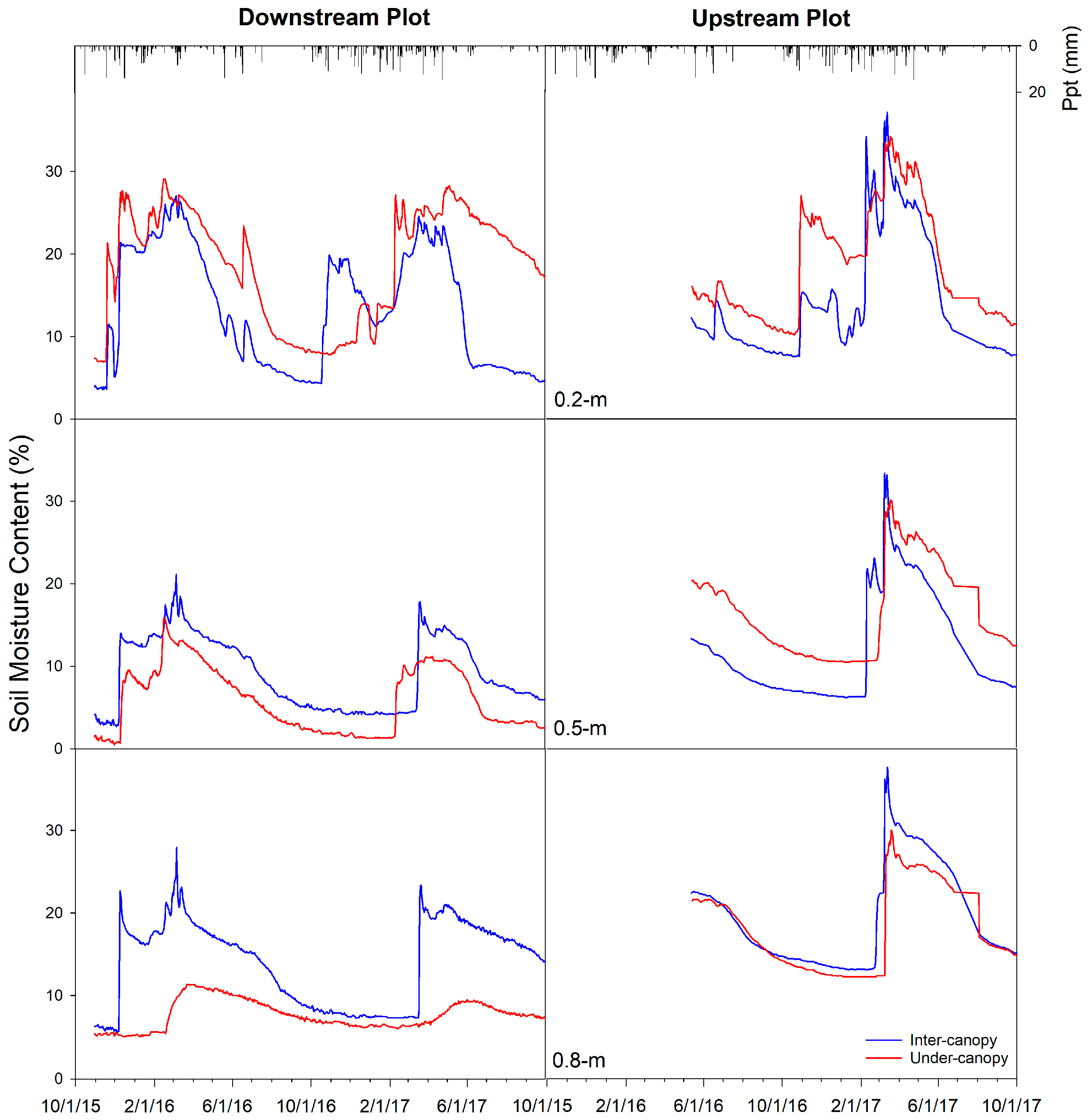
A seasonal θ response to precipitation inputs was observed in the Jensen WS plots at all sensor depths. Figure 4 shows daily-averaged θ for the three different sensor depths (0.2, 0.5, and 0.8 m) at under-canopy and inter-canopy locations in both plots. Greater θ values were observed at the peak of the snowmelt runoff season in spring. The limited summer precipitation characteristic of the region was reflected in the decreasing θ values at all sensor locations during the dry season, reaching their lowest θ in fall and winter. The potential effects of tree canopy interception on θ were more evident in the deeper soil profile in the downstream plot. Greater θ levels were obtained at the inter-canopy location for both the 0.5 and 0.8 m sensor depths in this downstream plot. This may be due in part to higher sand content values at all depths at this location (Table A1). The effects of tree canopy interception on topsoil moisture were observed during periods of rain and early snowmelt runoff in January 2017. For example, greater θ levels were observed in the downstream plot for the 0.2 m sensor depth in the inter-canopy location in the fall of 2016. However, greater θ levels at the 0.2 m depth were generally observed most of the time for the under-canopy location in both plots (Figure 4).
The results from the ANOVA test showed there are significant θ differences (p ≤ 0.05) between inter- and under-canopy locations for most sensor depths in both plots. The exceptions were at the upstream plot, where no significant differences in θ between inter-canopy and under-canopy locations were found for the 0.8 m sensor depth.
3.2. Surface Water and Groundwater Relations—Watershed Scale
3.2.1. Precipitation and Streamflow
Total amount of precipitation recorded by the automated rain gauges averaged 230, 330, 316, and 381 mm in the last four years evaluated, 2014, 2015, 2016 and 2017, respectively. Peak snowpack depth ranged from 0.1 m in 2015 to 0.6 m in 2016. Year 2014 was considered a dry year for both rain and snow precipitation; year 2015 was mostly dominated by rain, and snow precipitation was low; year 2016 was below average for rain but received more snowfall than the other years evaluated; year 2017 showed a significant amount of both rain and snow, and total rainfall was above the average (358 mm) for the study site.
Greater streamflow in response to precipitation inputs was observed in the Mays WS during the four years evaluated when compared to Jensen WS. For the Mays WS, total annual streamflow volume was 882, 27,972, 27,753, and 72,035 m3 in years 2014 through 2017, respectively. For the Jensen WS, total streamflow volume was negligible in 2014 and 2015, and 51.6 and 35,278 m3 in 2016 and 2017, respectively. The average of total annual streamflow volume recorded over the last four years in Mays WS (32,161 m3) was 3.6 times greater than the average of total annual streamflow volume recorded over the last four years in Jensen WS (8832 m3). During the pre-treatment years (1995–2005), average annual streamflow volume in Mays WS was 1.8 times greater than in Jensen WS. Annual streamflow during the pre-treatment period ranged from 0 to 30,368 m3 in Mays WS and from 0 to 16,035 m3 in Jensen WS [45,47].
Snowpack and streamflow relationships during the years 2016 and 2017, when greater snowpack depths were observed, are illustrated in Figure 5. In 2016, snowpack depth rose to 0.4 m at Mays WS (treated) and to 0.6 m at Jensen WS (untreated) in mid-January and remained at that level until early February when it started melting. The snowmelt period that started in mid-February in 2016 generated almost an immediate streamflow response in Mays WS but not in Jensen WS. For Mays WS, streamflow peaked at 440 L min−1 on 3 March. For Jensen WS, streamflow peaked at 24 L min−1 on 1 March. In year 2017, snowpack began to build in early December and rose to 0.5 meters by mid-January in both Jensen WS and Mays WS. Snowpack in both watersheds persisted until early March when snow began melting, and within two weeks, the snowpack was negligible in both watersheds. Streamflow peaked at 1020 L min−1 for Mays WS on 19 March. For Jensen WS, streamflow peaked at 687 L min−1 on 17 March (Figure 5).
Snowmelt runoff resulted in transient surface and subsurface flow connections in the stream in Mays WS. For example, Figure 6 shows streamflow response to the 2016 and 2017 snowmelt runoff seasons along the stream draining out of Mays WS. In the well installed in the streambed at the watershed outlet, the first response was observed below the surface on 11 February 2016. Water level rose sharply and peaked 7.5 cm above streambed surface on 19 February, then water level fluctuated above and below the surface until the end of April when it began a steady decline. The first response of the downstream well, located 1000 m downstream, was observed on 16 February. Water level in this well peaked at 0.5 m above streambed surface on 5 March, and remained above the surface for about three weeks until it dropped to baseflow conditions on 9 April 2016. In year 2017, the first response in the outlet well was observed below the surface on 25 February; water level peaked at 0.23 m above streambed surface on 16 March 2017, then returned to baseflow conditions on 2 May 2017. The first response in the downstream well was observed on 10 March, peaked at 0.7 m above streambed surface on 16 March, then returned to baseflow conditions on 14 April 2017 (Figure 6).
3.2.2. Precipitation and Springflow
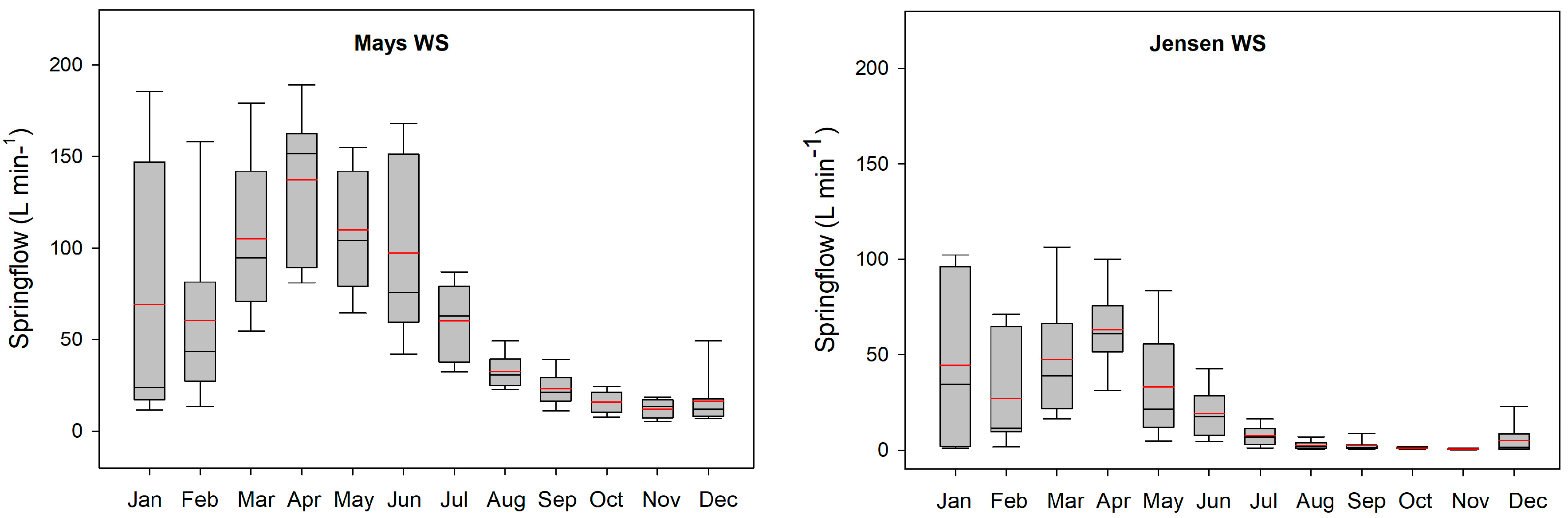
Greater springflow was observed in the Mays WS (treated) when compared to the Jensen WS (untreated). Figure 7 shows that springflow in both watersheds followed a seasonal pattern corresponding to regional precipitation dynamics (dry summers, wet winters). In general, springflow began increasing in late winter, peaked in mid-spring, and then followed a steady decline until reaching baseline levels in late summer.
During the period (2004–2017) evaluated, springflow rates ranged from 5 to 190 L min−1 in Mays WS and from 0 to 110 L min−1 in Jensen WS. During the pre-treatment years (2004–2005), mean springflow (L min−1) in Mays WS (49.3 ± 7.8) was three times greater than in Jensen WS (16.4 ± 3.4). The difference in springflow between the two watersheds increased during the post treatment years (2007–2017) when mean springflow in Mays WS (61.1 ± 5.1) was five times greater than in Jensen WS (12.1 ± 2.1). During the year of the treatment, when juniper removal was taking place (2006), mean springflow in Mays WS was 91.9 (±11.7) and in Jensen 40.6 (±8.0) L min−1.
Springflow rates during the last two years evaluated were at near maximum levels observed during the entire period of record (2004–2017). For the year 2017, springflow rates were highest in March in both watersheds and were measured at 187 L min−1 in Mays WS and at 109 L min−1 in Jensen WS. For the year 2016, springflow rates were highest in mid-April and were measured at 189 L min−1 in Mays WS and at 76 L min−1 in Jensen WS.
3.2.3. Soil Moisture and Shallow Groundwater Level Fluctuations
Similar to that observed in the under-canopy and inter-canopy locations in the Jensen WS plots in 2016 and 2017, a seasonal response to precipitation was observed in the other soil moisture stations in both Mays WS and Jensen WS over a 4-year period. Figure 8 illustrates the seasonal pattern of daily-averaged θ fluctuations collected from the monitoring stations installed at upper and lower locations in each watershed (see Figure 1). Greater θ levels were observed during the bulk of the snowmelt runoff season every year across soil stations and sensor depth. This was particularly evident at the deepest soil sensor depth from March through May where we found θ in 2014 was significantly lower (p ≤ 0.05) compared to each of the other three years evaluated except for the upper station in the Mays WS in 2017.
Groundwater level in all wells began rising with onset of winter precipitation, reached its peak level in spring, then followed a steady decline until it returned to baseline conditions in mid to late summer. Most upland wells went dry at 8 or 9 m depth below ground surface, except one well in the treated watershed that has remained at relatively high groundwater levels since it was installed in 2005. The three wells in the Riparian Valley had a steady groundwater level rise following installation in October 2014 and have remained at relatively high levels ever since.
Figure 9 shows four years of snowpack depth in Jensen WS and shallow aquifer fluctuations in both watersheds and in the Riparian Valley. It can be observed that snowpack accumulation was considerably higher in 2016 and 2017 than in years 2014 and 2015. Also, groundwater level rises were considerably higher in the Jensen WS and Riparian Valley well locations in 2016 and 2017 when compared to previous years. Peak groundwater-level rises over 5 m were observed in Jensen WS during the snowmelt runoff season in years 2016 and 2017. Early in the aquifer recharge season, a relatively rapid groundwater level rise and decline pattern was observed in Mays WS during most years evaluated. The location of the Mays WS wells in mostly fractured rock substrate may have contributed to the quick transport of groundwater out of the site that resulted in less pronounced groundwater mounds observed during the aquifer recharge season. A faster response and a higher groundwater level peak were observed in the Riparian Valley well in 2016 and 2017 when compared to the response in the previous, drier, year 2015. Soil moisture content in the Riparian Valley remained at or near saturation levels since sensor installation in the spring of 2016 and that was reflected in the groundwater level fluctuations observed during the last two years at this site.
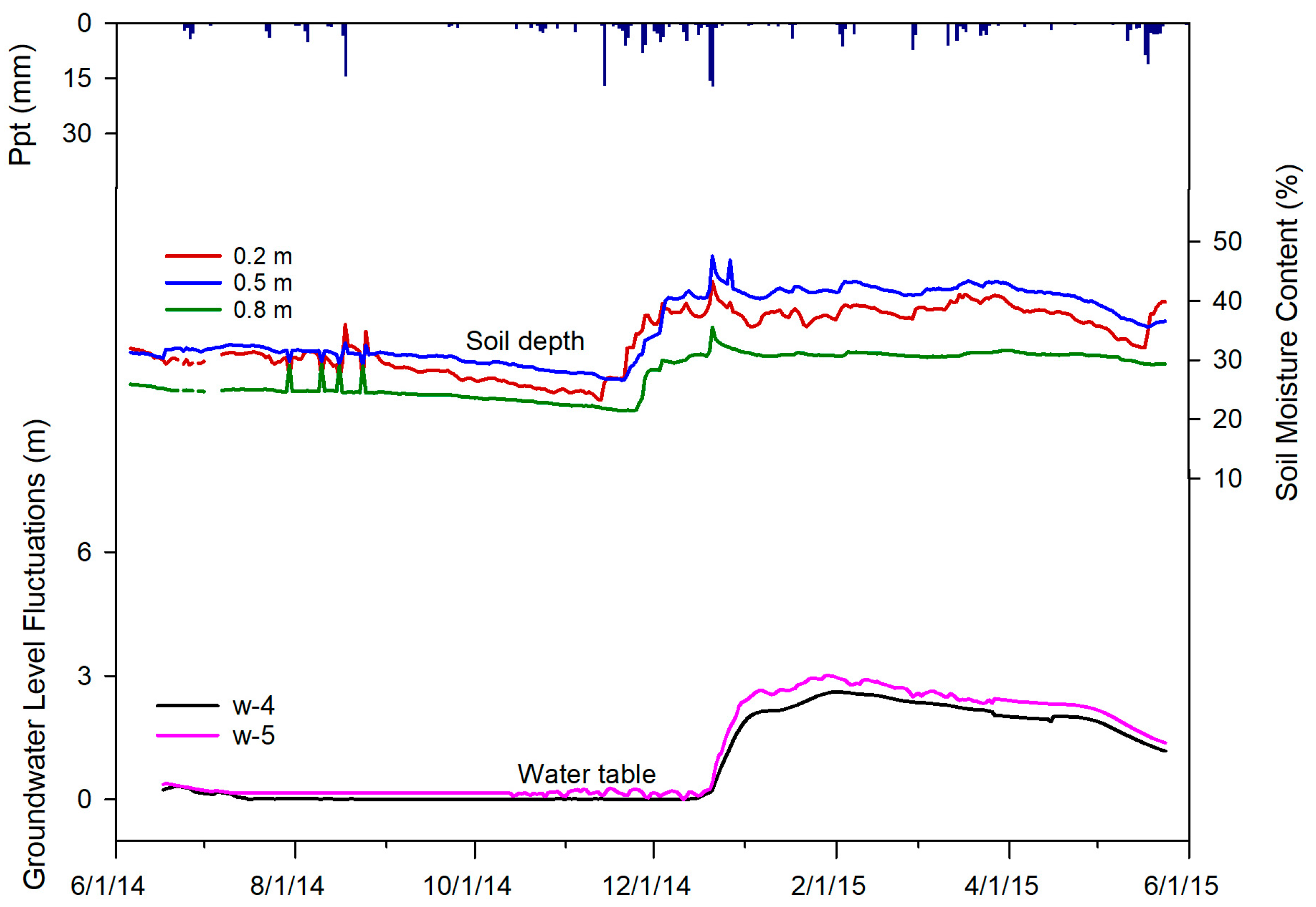
A closer look at precipitation, soil moisture, and shallow groundwater relationships in Jensen WS during June 2014 through June 2015 is illustrated in Figure 10. It can be observed that summer precipitation had an effect on θ levels but not on groundwater. Winter precipitation considerably increased θ levels at all sensor depths and had an effect on shallow groundwater level response three weeks after θ increased in the deepest soil sensor at 0.8 m. Groundwater level fluctuations in the transect wells, as illustrated by wells w-4 and w-5, peaked at the end of January and stayed above two meters for most of the winter and spring, until they started declining in May (Figure 10). A similar response was observed during all four years (2014–2017) evaluated in the two watersheds. The hydrologic connections between soil moisture and groundwater were less evident in the Riparian Valley due to near saturation conditions (data not shown) during and following sensor installation in the spring of 2016.
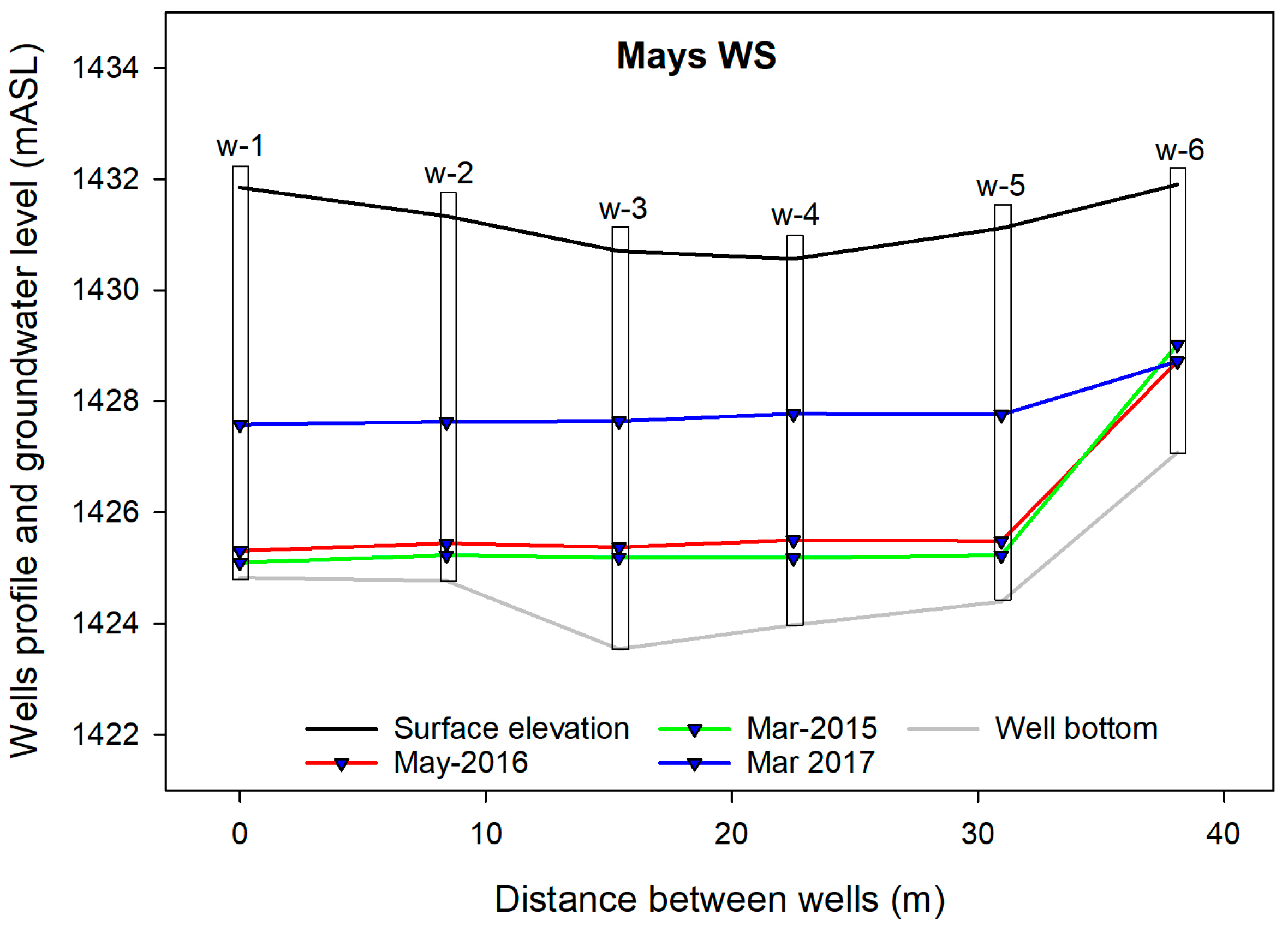
Figure 11 shows a cross-sectional view of groundwater level fluctuations along the 6-well transect installed in each watershed. Manual measurements of depth to water table, depth to well bottom, and soil surface elevation were used to construct the cross-sectional profile in each watershed. The bottom of all wells are at, or very close to, bedrock level, thus it reflects a significant section of the underground channel profile at the outlet of each watershed. Depth to water table was substantially shallower in March 2017 when compared to the March 2015 and May 2016 readings in all but w-6 in Mays WS. Since juniper removal, w-6 in Mays WS has consistently remained at shallower groundwater depth than the rest of the wells in that transect, this was also shown during the three different dates evaluated. The highest water table levels were observed in March 2017 when a depth to water table of 3.2 m was measured in w-4 in Mays WS and w-5 in Jensen WS. This contrasts with the lower water table levels observed in March 2015 when depth to water table was 6.8 m in w-1 in Mays WS and was at 6 m depth in w-6 in Jensen WS (Figure 11).
4. Discussion
This study shows that strong seasonal connections between surface and subsurface flows exist in rangeland watershed systems of semiarid central Oregon. Hydrologic connections such as the ones reported in this study can be affected by a combination of biotic and abiotic factors including overstory vegetation, precipitation, soils, geology, and topographic gradient [36,37,38,39].
Multiple processes (e.g., infiltration) are negatively affected when western juniper crosses the threshold from co-dominant to dominant species, which is around 30% canopy cover [8]. The high levels of juniper encroachment observed in the untreated watershed (Jensen WS) resulted in average interception losses of up to 46% of total precipitation in one of the plots. Overall, for the 0.5 and 0.8 depths, greater soil moisture content levels were found at inter-canopy versus under-canopy locations. We found that top (0.2 m) soil moisture was generally higher in under-canopy vs. inter-canopy locations except during fall precipitation in the downstream plot. These results are different from those of a study conducted in western juniper woodlands of Idaho where no statistical differences in shallow (0.15 m) soil moisture levels were found between under-canopy and inter-canopy locations [56]. We theorized that the greater soil moisture levels we found at shallow locations under the canopy can be in part attributed to the shading provided by the trees that may have resulted in less soil evaporation.
We observed that the connections between surface and subsurface water flows occurred through most of winter precipitation and spring snowmelt-runoff seasons. Timing and amount of precipitation heavily influenced soil moisture and shallow aquifer response across the landscape. Soil moisture recharge in response to precipitation inputs in winter was followed by a relatively rapid water table rise that peaked during the spring. Greater snowpack depths observed in the last two years resulted in greater groundwater level response in both watersheds and in the riparian valley. Streamflow and springflow rates in response to snowmelt runoff were considerably higher in the treated watershed (Mays WS; juniper removed 2006) when compared to the untreated Jensen WS. During the pre-treatment years, streamflow in Mays WS was 1.8 times greater than in Jensen WS. For the last four years evaluated (2013–2017), streamflow in the treated Mays WS averaged 3.6 times more than in the untreated Jensen WS. Springflow in Mays WS was three times greater than in Jensen WS during the pre-treatment years. After juniper removal, springflow increased in the Mays WS averaging five times more than in Jensen WS. Precipitation that occurred during the summer generally increased soil moisture levels but this was not reflected in stream or groundwater flow.
Most studies related to hydrologic connectivity have been conducted in steep mountains with shallow soils and narrow valley floors; it remains an open question what the dynamics of hydrologic connections are in areas with lower topographic relief [33]. The relatively low topographic relief and underlying geology characteristic of our study site create the conditions for transient underground storage and slow release through the shallow aquifer (<10 m) system [57]. Results show that springflow and shallow groundwater response continued beyond the time that streamflow was observed in both watersheds. The increased subsurface flow residence time may have contributed to prolong the hydrologic connections between the watersheds and the downstream valley. This was reflected in the riparian wells where the seasonal groundwater level response extended past that which was observed in the wells in both upland watersheds. An ongoing study we are conducting where we use isotope tracers to identify water sources in these watershed systems shows there are close similarities between surface and subsurface water flow sources, which further points to the connective nature of the upland water sources and the downstream valley [46]. A relatively rapid groundwater level rise and decline pattern was observed in the wells in the treated watershed. We attributed the rapid groundwater level rise and declines observed to the wells being located in mostly fractured rock substrate, conditions that may have resulted in less pronounced groundwater mounds and quick transport of groundwater out of the site.
Results from this study conducted in a 358 mm annual precipitation site indicate that precipitation reaching the ground can rapidly percolate through the soil profile and into the shallow aquifer, and that strong hydrologic connections between uplands and downstream valleys exist during winter precipitation and snowmelt runoff seasons. This study enhances base knowledge of the interconnectedness of ecohydrologic features in rangeland watershed systems of the western United States. Similar winter precipitation and shallow aquifer conditions can be found in other juniper-dominated rangelands in Oregon and the Pacific Northwest Region in the U.S in general. This offers a good opportunity to further explore vegetative manipulation effects on ecosystem services such as water and forage provisioning. Results from this study can contribute to improved natural resource management through a better understanding of surface water and groundwater relations in rangeland ecosystems and the role that woody vegetation encroachment may have on altering ecohydrologic processes. Further work is needed to integrate and expand plot and watershed scale findings to the larger regional scale.
Acknowledgments
The authors gratefully acknowledge the continuous support of the Hatfield High Desert Ranch, the U.S. Department of Interior Bureau of Land Management—Prineville Office, and the OSU’s Extension Service, in this research effort. Our thanks go to John Buckhouse, Michael Fisher, and Mike Borman who had provided critical guidance throughout this long-term study journey. Also, we want to thank the multiple graduate and undergraduate students from Oregon State University, and volunteers, who participated in various field data collection activities related to the results here presented. This study was funded in part by NSF-STEM Scholarship Program, the Oregon Beef Council, the Oregon Watershed Enhancement Board, the Oregon Agricultural Research Foundation, and the Oregon Agricultural Experiment Station.
Author Contributions
Carlos G. Ochoa, Phil Caruso, Grace Ray, and Tim Deboodt conducted field data collection and analyses. Carlos G. Ochoa and Tim Deboodt developed the study design. W. Todd Jarvis and Steven J. Guldan provided expert knowledge used in data analysis and interpretation. All co-authors contributed to the writing of the manuscript.
Conflicts of Interest
The authors declare no conflict of interest.
Appendix A
Soil Physical Properties
Soil bulk density and soil texture varied across study sites. For both watersheds, soil texture was classified as sandy clay loam at all sampling depths. Soil clay content increased with depth for the Riparian Valley site, from silt loam (0.2 m), to silty clay loam (0.5 m) to clay (0.8 m) (Table A1). Higher sand content values at all depths were obtained for the downstream location in the alluvium valley of the Jensen WS (untreated). Soil bulk density ranged from 0.93 Mg m−3 in the Riparian Valley to 1.60 Mg m−3 in the Mays WS (treated).

Table A1.
Soil physical properties for the three sites within the study area, (a) Mays WS, (b) Jensen WS, and (c) Riparian Valley, showing the mean and standard error (n = 3) of soil bulk density and soil particle distribution of sand, silt, and clay at each soil depth. The Jensen WS location illustrates data collected at under-canopy and inter-canopy areas in upstream and downstream settings. N/A = Data not available.
| Soil Depth | Bulk Density | Sand | Silt | Clay |
|---|---|---|---|---|
| (Mg m−³) | (%) | (%) | (%) | |
| (a) Mays WS | ||||
| 0.2 m | 1.51 ± 0.001 | 67.5 ± 1.93 | 11.2 ± 0.94 | 21.3 ± 0.99 |
| 0.5 m | 1.60 ± 0.04 | 69.6 ± 0.00 | 9.2 ± 0.00 | 21.2 ± 0.00 |
| 0.8 m | 1.55 ± 0.02 | 68.9 ± 0.54 | 9.9 ± 0.27 | 21.2 ± 0.47 |
| (b) Jensen WS | ||||
| Upstream—Under-canopy | ||||
| 0.2 m | 1.18 ± 0.04 | 59.1 ± 1.46 | 11.7 ± 0.24 | 29.3 ± 1.23 |
| 0.5 m | 1.36 ± 0.03 | 62.4 ± 0.98 | 11.3 ± 0.85 | 26.3 ± 0.88 |
| 0.8 m | 1.53 ± 0.06 | 60.5 ± 0.44 | 12.9 ± 0.54 | 26.5 ± 0.85 |
| Upstream—Inter-canopy | ||||
| 0.2 m | 1.29 ± 0.02 | 65.2 ± 1.15 | 13.6 ± 0.50 | 21.2 ± 1.54 |
| 0.5 m | 1.46 ± 0.04 | 62.7 ± 0.54 | 14.8 ± 0.50 | 22.5 ± 0.61 |
| 0.8 m | 1.57 ± 0.01 | 62.0 ± 0.00 | 16.4 ± 0.00 | 21.6 ± 0.00 |
| Downstream—Under-canopy | ||||
| 0.2 m | N/A | 81.1 ± 1.44 | 16.5 ± 0.99 | 2.5 ± 0.52 |
| 0.5 m | N/A | 74.4 ± 0.94 | 15.5 ± 1.29 | 10.1 ± 0.77 |
| 0.8 m | N/A | 75.7 ± 1.09 | 16.1 ± 0.72 | 8.2 ± 1.70 |
| Downstream—Inter-canopy | ||||
| 0.2 m | N/A | 78.4 ± 0.94 | 15.4 ± 1.25 | 6.2 ± 2.16 |
| 0.5 m | N/A | 79.1 ± 2.18 | 14.1 ± 1.91 | 6.9 ± 0.27 |
| 0.8 m | N/A | 79.1 ± 2.37 | 12.1 ± 1.36 | 8.9 ± 1.52 |
| (c) Riparian Valley | ||||
| 0.2 m | 0.93 ± 0.04 | 24.4 ± 5.95 | 59.8 ± 1.73 | 15.8 ± 4.33 |
| 0.5 m | 1.00 ± 0.04 | 19.2 ± 3.46 | 57.1 ± 3.05 | 23.7 ± 2.57 |
| 0.8 m | 0.97 ± 0.01 | 34.7 ± 0.054 | 20.9 ± 2.25 | 44.4 ± 2.66 |
References
- Hoffman, M.T.; Cowling, M. Vegetation change in the semi-arid Karoo over the last 200 years: An expanding Karoo—Fact or fiction. S. Afr. J. Sci. 1990, 86, 286–294. [Google Scholar]
- Puttock, A.; Dungait, J.A.J.; Macleod, C.J.A.; Bol, R.; Brazier, R.E. Woody plant encroachment into grasslands leads to accelerated erosion of previously stable organic carbon from dryland soils. J. Geophys. Res. Biogeosci. 2014, 119, 2345–2357. [Google Scholar] [CrossRef] [Green Version]
- Scholes, R.J.; Archer, S.R. Tree-Grass Interactions in Savannas. Annu. Rev. Ecol. Syst. 1997, 28, 517–544. [Google Scholar] [CrossRef]
- Ratajczak, Z.; Nippert, J.B.; Collins, S.L. Woody encroachment decreases diversity across North American grasslands and savannas. Ecology 2012, 93, 697–703. [Google Scholar] [CrossRef] [PubMed]
- Millennium Ecosystem Assessment. Ecosystems and Human Well-Being: Desertification Synthesis; World Resources Institute: Washington, DC, USA, 2005. [Google Scholar]
- Intergovernmental Panel on Climate Change (IPCC). Climate Change 2014: Synthesis Report; Contribution of Working Groups I, II and III to the Fifth Assessment Report of the Intergovernmental Panel on Climate Change; Core Writing Team, Pachauri, R.K., Meyer, L.A., Eds.; IPCC: Geneva, Switzerland, 2014; 151p. [Google Scholar]
- Romme, W.H.; Allen, C.D.; Bailey, J.D.; Baker, W.L.; Bestelmeyer, B.T.; Brown, P.M.; Eisenhart, K.S.; Floyd, M.L.; Huffman, D.W.; Jacobs, B.F.; et al. Historical and modern disturbance regimes, stand structures, and landscape dynamics in piñon–juniper vegetation of the Western United States. Rangel. Ecol. Manag. 2009, 62, 203–222. [Google Scholar] [CrossRef]
- Miller, R.F.; Bates, J.D.; Svejcar, T.J.; Pierson, F.B.; Eddleman, L.E. Biology, Ecology, and Management of Western Juniper (Juniperus occidentalis); Technical Bulletin; Agricultural Experiment Station, Oregon State University: Corvallis, OR, USA, 2005; Volume 152. [Google Scholar]
- Miller, R.F.; Tausch, R.J. The role of fire in juniper and pinyon woodlands: A descriptive analysis. In Proceedings of the Invasive Species Workshop: The Role of Fire in the Control and Spread of Invasive Species. Held at Fire Conference 2000: The First National Congress on Fire Ecology, Prevention, and Management; Misc. Pub. 11; Galley, K.E.M., Wilson, T.P., Eds.; Tall Timbers Research Station: Tallahassee, FL, USA, 2001. [Google Scholar]
- Cowlin, R.W.; Briegleb, P.A.; Moravets, F.L. Forest Resources of the Ponderosa Pine Region of Washington and Oregon; U.S. Department of Agriculture, Forest Service: Washington, DC, USA, 1942.
- Azuma, D.L.; Hiserote, B.A.; Dunham, P.A. The Western Juniper Resource of Eastern Oregon; Resources Bulletin, PNW-RB-249; USDA, Forest Service, Pacific Northwest Research Station: Portland, OR, USA, 2005; 18p.
- Burns, R.M.; Honkala, B.H. Tech. Coords. Silvics of North America: 1. Conifers; 2. Hardwoods. In Agriculture Handbook 654; U.S. Department of Agriculture, Forest Service: Washington, DC, USA, 1990; Volume 2, p. 877. [Google Scholar]
- Gedney, D.R.; Azuma, D.L.; Bolsinger, C.L.; McKay, N. Western Juniper in Eastern Oregon; Gen. Tech. Rep. PNW-GTR-464; U.S. Department of Agriculture, Forest Service, Pacific Northwest Research Station: Portland, OR, USA, 1999; 53p.
- Chambers, J.C. Pinus monophylla establishment in an expanding Pinus-Juniperus woodland: Environmental conditions, facilitation and interacting factors. J. Veg. Sci. 2001, 12, 27–40. [Google Scholar] [CrossRef]
- Coppedge, B.R.; Engle, D.M.; Masters, R.E.; Gregory, M.S. Predicting juniper encroachment and CRP effects on avian community dynamics in southern mixed-grass prairie, USA. Biol. Conserv. 2004, 115, 431–441. [Google Scholar] [CrossRef]
- Taylor, C.A. Role of summer prescribed fire to manage shrub-invaded grasslands. In Proceedings of the Shrubland Dynamics—Fire and Water, Lubbock, TX, USA, 10–12 August 2004; RMRS-P-47; Sosebee, R.E., Wester, D.B., Britton, C.M., McArthur, E.D., Kitchen, S.G., Eds.; US Department of Agriculture, Forest Service: Fort Collins, CO, USA, 2007; pp. 52–55. [Google Scholar]
- Gottfried, G.J.; Pieper, R.D. Pinyon-juniper rangelands. In Livestock Management in the American Southwest: Ecology, Society, and Economics; Jemison, R., Raish, C., Eds.; Elsevier: New York, NY, USA, 2000; pp. 153–212. [Google Scholar]
- McPherson, G.R.; Wright, H.A. Effects of cattle grazing and juniperus pinchotii canopy cover on herb cover and production in western Texas. Am. Midl. Nat. 1990, 123, 144–151. [Google Scholar] [CrossRef]
- Vaitkus, M.R.; Eddleman, L.E. Composition and Productivity of a Western Juniper Understory and Its Response to Canopy Removal. In Proceedings—Pinyon-Juniper Conference; USDA-Forest Service Gen. Tech. Rep. INT-215; Everett, R.L., Ed.; Intermountain Research Station: Ogden, UT, USA, 1987; pp. 456–460. [Google Scholar]
- Tausch, R.J.; West, N.E. Plant species composition patterns with differences in tree dominance on a southwestern Utah pinyon-juniper site. In Desired Future Conditions for Pinyon-Juniper Ecosystems; Gen. Tech. Rep. RM-GTR-258; US Department of Agriculture, Forest Service: Flagstaff, AZ, USA, 1995; pp. 16–23. [Google Scholar]
- Miller, R.F.; Svejcar, T.J.; Rose, J.A. Impacts of western juniper on plant community composition and structure. J. Range Manag. 2000, 53, 574–585. [Google Scholar] [CrossRef]
- Bates, J.D.; Miller, R.F.; Svejcar, T. Long-term successional trends following western juniper Cutting. Rangel. Ecol. Manag. 2005, 58, 533–541. [Google Scholar] [CrossRef]
- Bates, J.D.; Svejcar, T.J.; Miller, R.F. Effects of juniper cutting on nitrogen mineralization. J. Arid Environ. 2002, 51, 221–234. [Google Scholar] [CrossRef]
- Mollnau, C.; Newton, M.; Stringham, T. Soil water dynamics and water use in a western juniper (Juniperus occidentalis) woodland. J. Arid Environ. 2014, 102, 117–126. [Google Scholar] [CrossRef]
- Petersen, S.L.; Stringham, T.K. Infiltration, runoff, and sediment yield in response to western juniper encroachment in Southeast Oregon. Rangel. Ecol. Manag. 2008, 61, 74–81. [Google Scholar] [CrossRef]
- Wilcox, B.P. Runoff and erosion in intercanopy zones of pinyon-juniper woodlands. J. Range Manag. 1994, 47, 285–295. [Google Scholar] [CrossRef]
- Pierson, F.B.; Williams, C.J.; Kormos, P.R.; Al-Hamdan, O.Z. Short-term effects of tree removal on infiltration, runoff, and erosion in woodland-encroached sagebrush steppe. Rangel. Ecol. Manag. 2014, 67, 522–538. [Google Scholar] [CrossRef]
- Cline, N.L.; Roundy, B.A.; Pierson, F.B.; Kormos, P.; Williams, C.J. Hydrologic Response to Mechanical Shredding in a Juniper Woodland. Rangel. Ecol. Manag. 2010, 63, 467–477. [Google Scholar] [CrossRef]
- Allen, C.D. Ecohydrology of pinon-juniper woodlands in the Jemez Mountains, New Mexico: Runoff, erosion, and restoration. In Ecology, Management, and Restoration of Piñon-Juniper and Ponderosa Pine Ecosystems; U.S. Department of Agriculture, Forest Service, Rocky Mountain Research Station: Fort Collins, CO, USA, 2008; pp. 65–66. [Google Scholar]
- Hibbert, A.R. Water yield improvement potential by vegetation management on western rangelands. J. Am. Water Resour. Assoc. 1983, 19, 375–381. [Google Scholar] [CrossRef]
- Ffolliott, P.F.; Gottfried, G.J. Hydrological Processes in the Pinyon-Juniper Woodlands: A Literature Review; General Technical Report RMRS GTR-271; US Department of Agriculture, Forest Service, Rocky Mountain Research Station: Fort Collins, CO, USA, 2012.
- Kuhn, T.; Cao, D.; George, M. Juniper removal may not increase overall Klamath River Basin water yileds. Calif. Agric. 2007, 61, 166–171. [Google Scholar] [CrossRef]
- Barlow, P.M.; Leake, S.A. Streamflow Depletion by Wells—Understanding and Managing the Effects of Groundwater Pumping on Streamflow; U.S. Geological Survey Circular 1376; Department of the Interior, U.S. Geological Survey: Reston, VA, USA, 2012; 84p.
- Taylor, R.G.; Scanlon, B.; Döll, P.; Rodell, M.; van Beek, R.; Wada, Y.; Longuevergne, L.; Leblanc, M.; Famiglietti, J.S.; Edmunds, M.; et al. Ground water and climate change. Nat. Clim. Chang. 2013, 3, 322–329. [Google Scholar] [CrossRef] [Green Version]
- Sophocleous, M. Interactions between groundwater and surface water: The state of the science. Hydrogeol. J. 2002, 10, 52–67. [Google Scholar] [CrossRef]
- Detty, J.M.; McGuire, K.J. Topographic controls on shallow groundwater dynamics: Implications of hydrologic connectivity between hillslopes and riparian zones in a till mantled catchment. Hydrol. Process. 2010, 24, 2222–2236. [Google Scholar] [CrossRef]
- Devito, K.; Creed, I.; Gan, T.; Mendoza, C.; Petrone, R.; Silins, U.; Smerdon, B. A framework for broad-scale classification of hydrologic response units on the Boreal Plain: Is topography the last thing to consider? Hydrol. Process. 2005, 19, 1705–1714. [Google Scholar] [CrossRef]
- Jencso, K.G.; McGlynn, B.L.; Gooseff, M.N.; Wondzell, S.M.; Bencala, K.E.; Marshall, L.A. Hydrologic connectivity between landscapes and streams: Transferring reach- and plot-scale understanding to the catchment scale. Water Resour. Res. 2009, 45. [Google Scholar] [CrossRef]
- Ocampo, C.J.; Sivapalan, M.; Oldham, C. Hydrological connectivity of upland-riparian zones in agricultural catchments: Implications for runoff generation and nitrate transport. J. Hydrol. 2006, 331, 643–658. [Google Scholar] [CrossRef]
- Ochoa, C.G.; Guldan, S.J.; Cibils, A.F.; Lopez, S.C.; Boykin, K.G.; Tidwell, V.C.; Fernald, A.G. Hydrologic connectivity of head waters and floodplains in a semiarid watershed. J. Contemp. Water Res. Educ. 2013, 152, 69–78. [Google Scholar] [CrossRef]
- Albertson, J.D.; Kiely, G. On the structure of soil moisture time series in the context of land surface models. J. Hydrol. 2001, 243, 101–119. [Google Scholar] [CrossRef]
- Emanuel, R.E.; Hazen, A.G.; Mcglynn, B.L.; Jencso, K.G. Vegetation and topographic influences on the connectivity of shallow groundwater between hillslopes and streams. Ecohydrology 2013, 7, 887–895. [Google Scholar] [CrossRef]
- Jencso, K.G.; McGlynn, B.L. Hierarchical controls on runoff generation: Topographically driven hydrologic connectivity, geology, and vegetation. Water Resour. Res. 2011, 47. [Google Scholar] [CrossRef]
- Miller, R.F.; Chambers, J.C.; Pyke, D.A.; Pierson, F.B.; Williams, C.J. A Review of Fire Effects on Vegetation and Soils in the Great Basin Region: Response and Ecological Site Characteristics; Gen. Tech. Rep. RMRS-GTR-308; U.S. Department of Agriculture, Forest Service, Rocky Mountain Research Station: Fort Collins, CO, USA, 2013.
- Deboodt, T.L. Watershed Response to Western Juniper Control. Ph.D. Thesis, Oregon State University, Corvallis, OR, USA, 2008. [Google Scholar]
- Ray, G. Long-Term Ecohydrologic Response to Western Juniper (Juniperus occidentalis) Control in Semiarid Watersheds of Central Oregon: A Paired Watershed Study. Master’s Thesis, Oregon State University, Corvallis, OR, USA, 2015. [Google Scholar]
- Fisher, M.P. Analysis of Hydrology and Erosion in Small, Paired Watersheds in a Juniper-Sagebrush Area of Central Oregon. Ph.D. Thesis, Oregon State University, Corvallis, OR, USA, 2004. [Google Scholar]
- Cooperative Climatological Data Summaries, Western Regional Climate Center. Available online: http://www.wrcc.dri.edu/cgi-bin/cliMAIN.pl?or0501 (accessed on 25 November 2017).
- Soil Survey Staff Natural Resources Conservation Service, United States Department of Agriculture. Official Soil Series Descriptions. Available online: https://www.nrcs.usda.gov/wps/portal/nrcs/detail/soils/home/?cid=nrcs142p2_053587 (accessed on 24 December 2017).
- Gee, G.W.; Bauder, J.W. Particle-size analysis. In Methods of Soil Analysis. Part 1; ASA and SSSA: Madison, WI, USA, 1986; pp. 383–411. [Google Scholar]
- Blake, G.R.; Hartge, K.H. Bulk density. In Methods of Soil Analysis. Part 1; ASA and SSSA: Madison, WI, USA, 1986; pp. 363–375. [Google Scholar]
- Strickler, G.S. Use of the Densiometer to Estimate Density of Forest Canopy on Permanent Sample Plots; PNW Old Series Research Notes No. 180; U.S. Department of Agriculture, Forest Service, Pacific Northwest Forest and Range Experiment Station: Portland, OR, USA, 1959; pp. 1–5.
- Kilpatrick, F.; Schneider, V. Use of flumes in measuring discharge. In US Geological Survey Techniques and Methods, Book 3; U.S. Department of the Interior, Geological Survey: Reston, VA, USA, 1983; pp. 21–26. [Google Scholar]
- Young, J.A.; Evans, R.A.; Easi, D.A. Stem flow on western juniper (Juniperus occidentalis) trees. Weed Sci. 1984, 32, 320–327. [Google Scholar]
- Larsen, R.E. Interception and Water Holding Capacity of Western Juniper. Ph.D. Thesis, Oregon State University, Corvallis, OR, USA, 1993. [Google Scholar]
- Niemeyer, R.J.; Link, T.E.; Seyfried, M.S.; Flerchinger, G.N. Surface water input from snowmelt and rain throughfall in western juniper: Potential impacts of climate change and shifts in semi-arid vegetation. Hydrol. Process. 2016, 30, 3046–3060. [Google Scholar] [CrossRef]
- Caruso, P. Hydrogeologic Framework of an Area of Interest in the Southeast Deschutes Basin Oregon, USA. In Hydrogeology and Hydrologic Connectivity of a Semiarid Central Oregon Rangeland System. Master’s Thesis, Oregon State University, Corvallis, OR, USA, 2017. [Google Scholar]
Figure 1.
Map of the study area showing Mays WS, Jensen WS, and the Riparian Valley sites, indicating the location of different monitoring instrumentation used in this study.
Figure 1.
Map of the study area showing Mays WS, Jensen WS, and the Riparian Valley sites, indicating the location of different monitoring instrumentation used in this study.

Figure 2.
Schematic illustrating soil moisture sensor placement and soil sampling depth at under-canopy and inter-canopy locations in the upstream plot in Jensen WS.
Figure 2.
Schematic illustrating soil moisture sensor placement and soil sampling depth at under-canopy and inter-canopy locations in the upstream plot in Jensen WS.

Figure 3.
Satellite images illustrating juniper trees (outlined in yellow) in the downstream (A) and upstream (B) experimental plots.
Figure 3.
Satellite images illustrating juniper trees (outlined in yellow) in the downstream (A) and upstream (B) experimental plots.

Figure 4.
Daily-averaged precipitation and soil moisture content for the three different sensor depths (0.2, 0.5, and 0.8 m) at inter-canopy and under-canopy locations in both plots in the Jensen WS. x-axis indicates month/day/year.
Figure 4.
Daily-averaged precipitation and soil moisture content for the three different sensor depths (0.2, 0.5, and 0.8 m) at inter-canopy and under-canopy locations in both plots in the Jensen WS. x-axis indicates month/day/year.

Figure 5.
Snowpack depth and runoff discharge during 2016 and 2017 in both watersheds illustrating the relationship between snow melting and streamflow measured at each watershed. x-axis indicates month/day/year.
Figure 5.
Snowpack depth and runoff discharge during 2016 and 2017 in both watersheds illustrating the relationship between snow melting and streamflow measured at each watershed. x-axis indicates month/day/year.
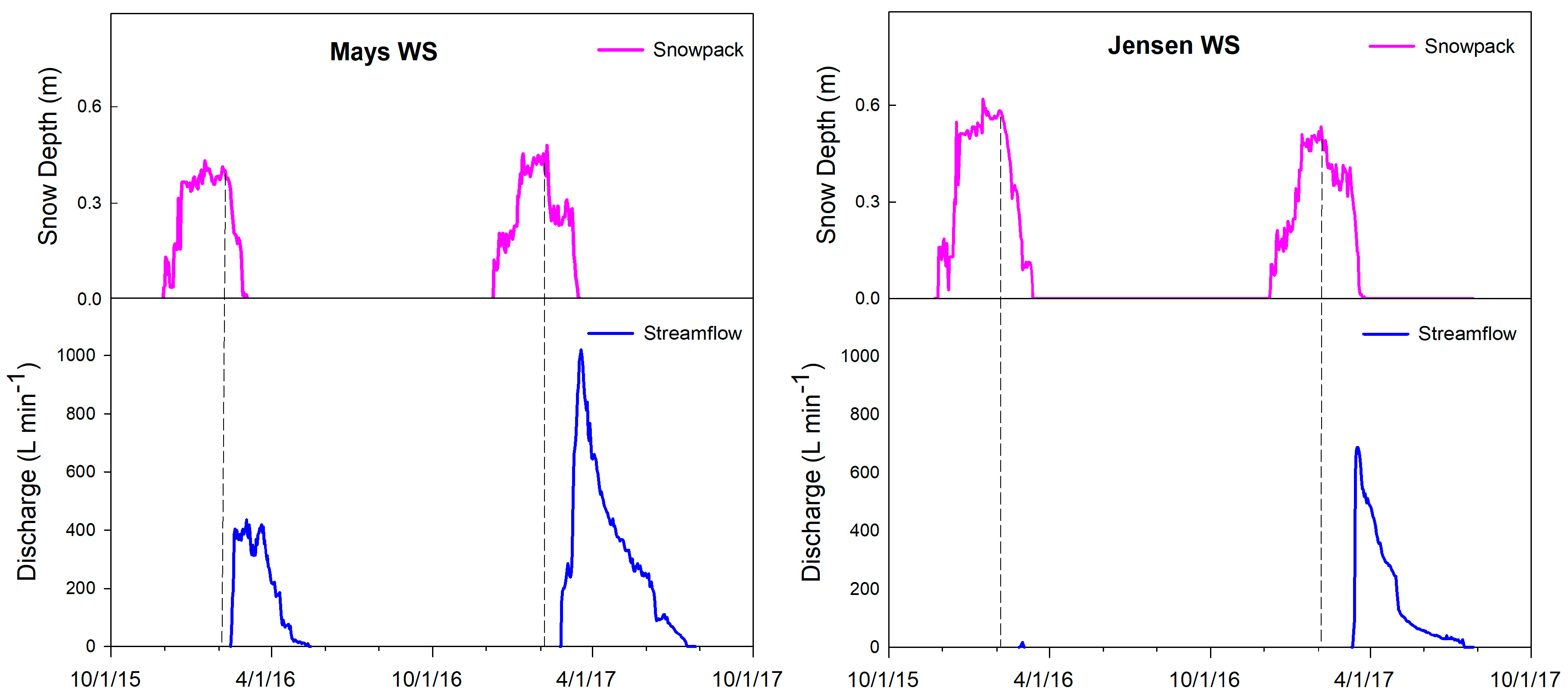
Figure 6.
Surface and subsurface stream water level response to snowmelt runoff at watershed outlet and downstream well locations in Mays WS in years 2016 and 2017. x-axis indicates month/day/year.
Figure 6.
Surface and subsurface stream water level response to snowmelt runoff at watershed outlet and downstream well locations in Mays WS in years 2016 and 2017. x-axis indicates month/day/year.
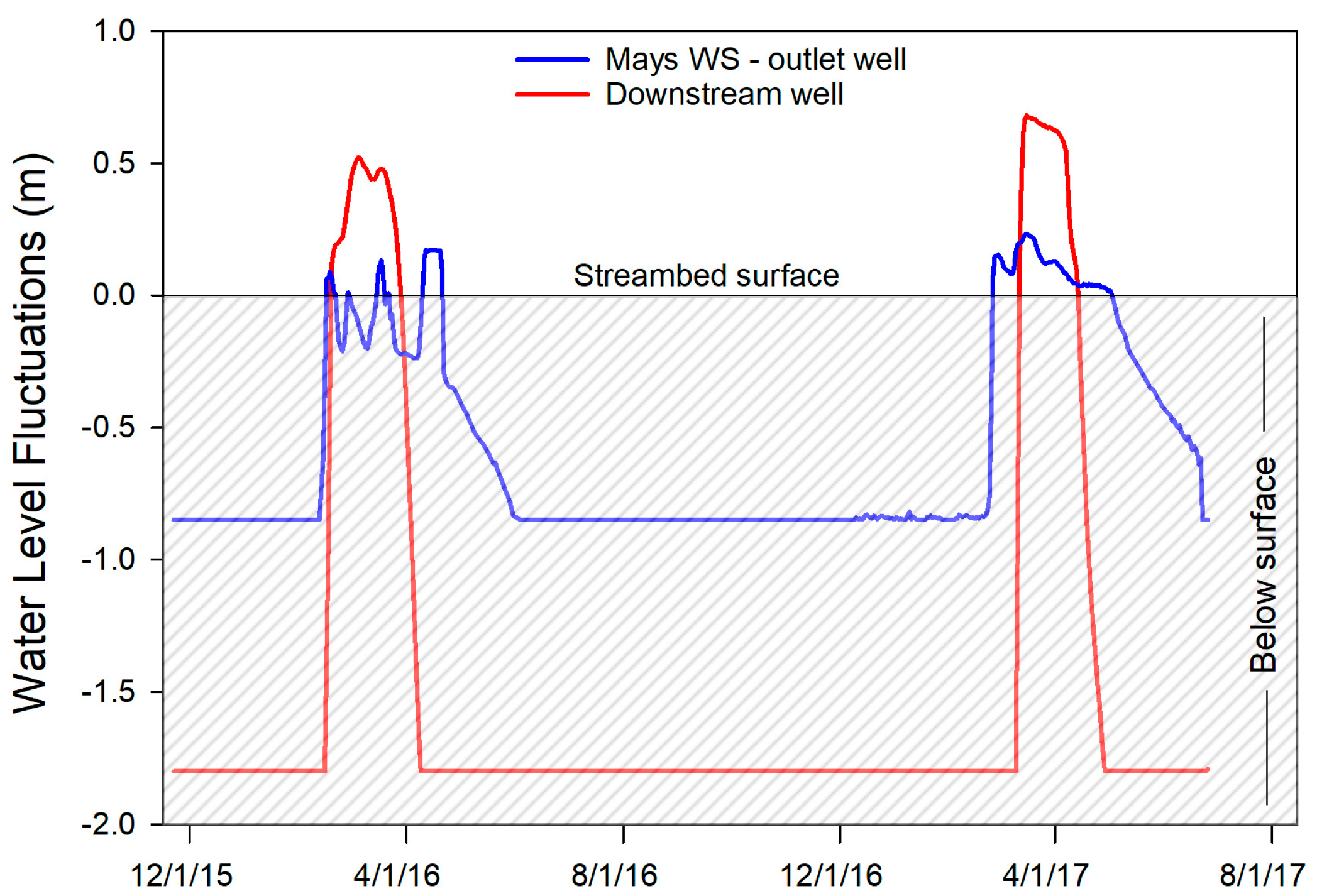
Figure 7.
Box diagram showing springflow rate estimates for both watersheds over the period of record September 2004 through November 2017. Each box diagram shows the mean (red line) and median (black line). The lower and upper ends of the boxes represent the 25th and 75th percentiles respectively. Lower and upper error bars represent the 10th and 90th percentiles, respectively.

Figure 8.
Soil moisture content fluctuations at different soil depths at upper and lower locations in both watersheds from 1 October 2013 through 27 July 2017. x-axis indicates month/day/year.
Figure 8.
Soil moisture content fluctuations at different soil depths at upper and lower locations in both watersheds from 1 October 2013 through 27 July 2017. x-axis indicates month/day/year.
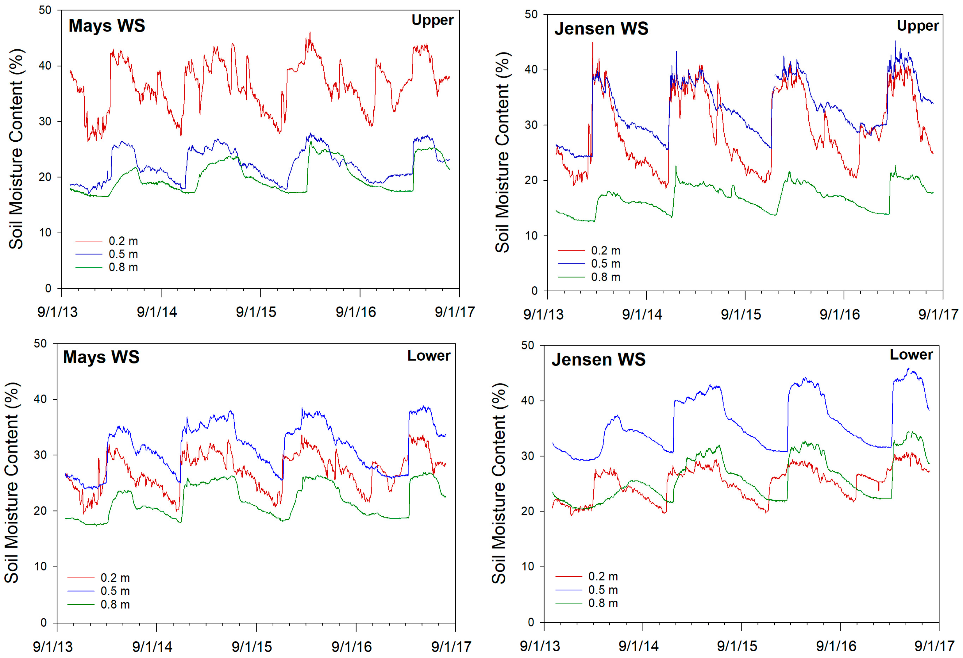
Figure 9.
Snowpack depth and seasonal water table fluctuations in selected wells in Mays WS and Jensen WS and in the Riparian Valley from October 2013 through May 2017. Flat lines at zero groundwater level depict wells were dry. x-axis indicates month/day/year.
Figure 9.
Snowpack depth and seasonal water table fluctuations in selected wells in Mays WS and Jensen WS and in the Riparian Valley from October 2013 through May 2017. Flat lines at zero groundwater level depict wells were dry. x-axis indicates month/day/year.
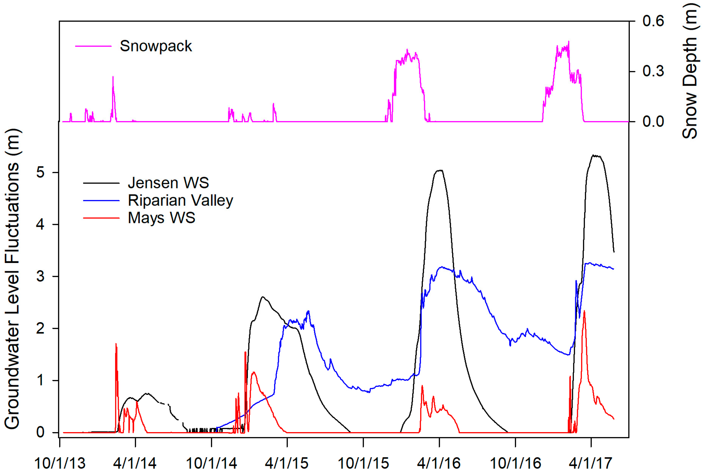
Figure 10.
Soil moisture and shallow groundwater level response to precipitation inputs in two wells (w-4 and w-5) in the well transect (see Figure 1) in Jensen WS during June 2014 through June 2015. x-axis indicates month/day/year.
Figure 10.
Soil moisture and shallow groundwater level response to precipitation inputs in two wells (w-4 and w-5) in the well transect (see Figure 1) in Jensen WS during June 2014 through June 2015. x-axis indicates month/day/year.

Figure 11.
Shallow groundwater levels at selected dates during runoff season in well-transects in both watersheds.
Figure 11.
Shallow groundwater levels at selected dates during runoff season in well-transects in both watersheds.

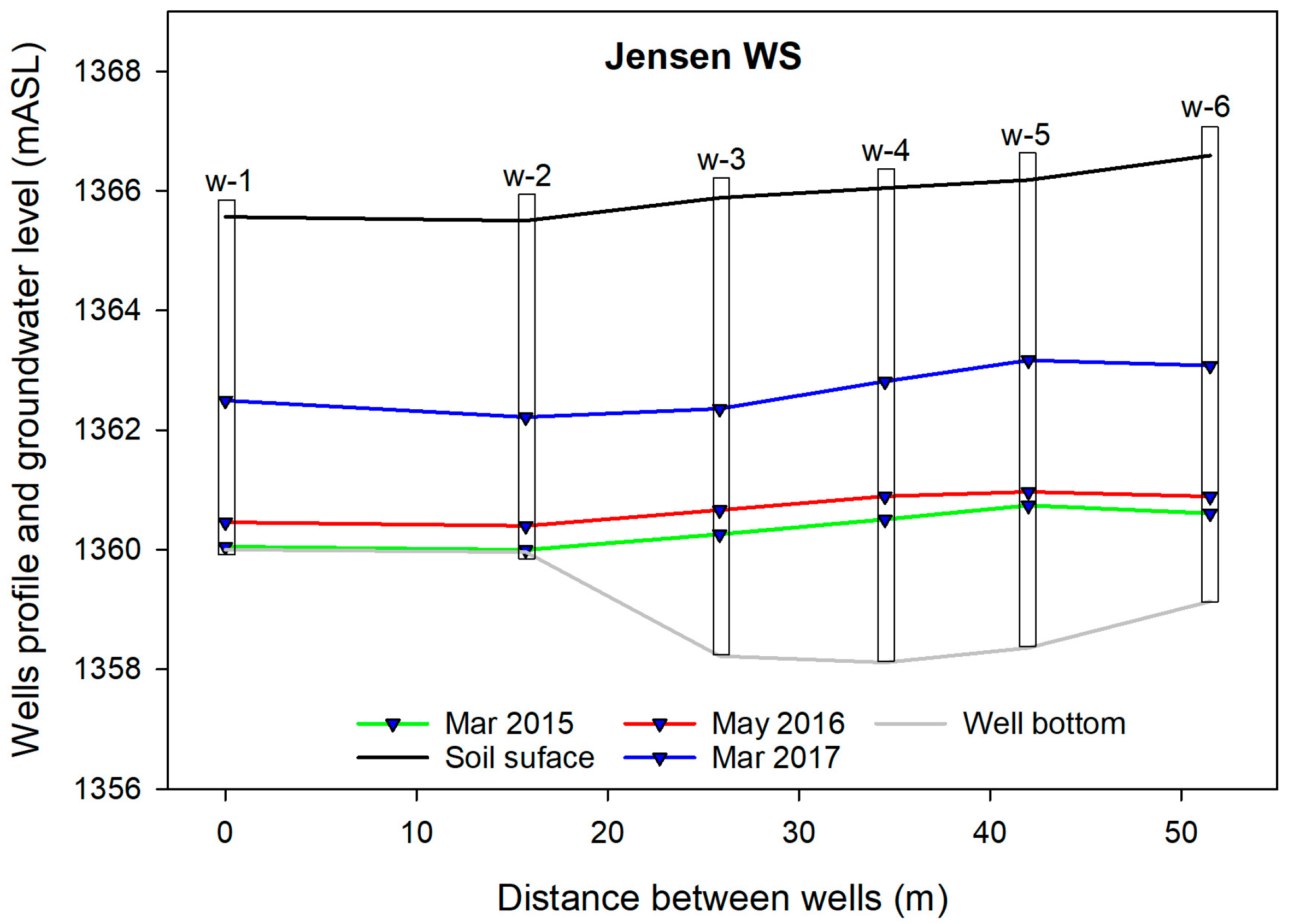
Table 1.
Tree canopy interception results for the two experimental plot sites, (a) Downstream and (b) Upstream, showing total precipitation (P), average interception for the entire plot (I), interception/precipitation ratio (I/P), and average interception and standard error for under-canopy (IUC), drip line (IDL), and inter-canopy (IIC) locations from October 2015 through March 2017. N/A = Data not available.
| Period of Record | P | I | I/P | Avg. IUC | Avg. IDL | Avg. IIC |
|---|---|---|---|---|---|---|
| (mm) | (mm) | (mm mm−1) | (mm) | (mm) | (mm) | |
| (a) Downstream | ||||||
| 31 October to 21 November 2015 | 24.4 | 8.2 | 0.34 | 17 ± 1.4 | 7 ± 0.1 | 0.5 ± 0.3 |
| 16 June to 17 September 2016 | 31.5 | 22.3 | 0.71 | 27 ± 2.6 | 25 ± 3.8 | 16 ± 0.2 |
| 18 September to 21 October 2016 | 34.0 | 15.0 | 0.44 | 30 ± 0.3 | 14 ± 1.5 | 0.3 ± 0.2 |
| 22 October to 10 November 2016 | 30.4 | 10.2 | 0.34 | 21 ± 1.0 | 9 ± 1.0 | 0.5 ± 0.1 |
| 11 November 2016 to 28 March 2017 | 267.4 | 123.1 | 0.46 | 191 ± 11.7 | 137 ± 3.6 | 42 ± 6.7 |
| (b) Upstream | ||||||
| 31 October to 21 November 2015 | N/A | N/A | N/A | N/A | N/A | N/A |
| 16 June to 17 September 2016 | N/A | N/A | N/A | N/A | N/A | N/A |
| 18 September to 21 October 2016 | N/A | N/A | N/A | N/A | N/A | N/A |
| 22 October to 10 November 2016 | 29.6 | 7.7 | 0.26 | 17.1 ± 3.2 | 6 ± 1.3 | 0.2 ± 0.04 |
| 11 November 2016 to 28 March 2017 | 278.0 | 127.2 | 0.46 | 192 ± 13.5 | 122 ± 8.0 | 68 ± 26.0 |
© 2018 by the authors. Licensee MDPI, Basel, Switzerland. This article is an open access article distributed under the terms and conditions of the Creative Commons Attribution (CC BY) license (http://creativecommons.org/licenses/by/4.0/).
Share and Cite
MDPI and ACS Style
Ochoa, C.G.; Caruso, P.; Ray, G.; Deboodt, T.; Jarvis, W.T.; Guldan, S.J. Ecohydrologic Connections in Semiarid Watershed Systems of Central Oregon USA. Water 2018, 10, 181. https://doi.org/10.3390/w10020181
AMA Style
Ochoa CG, Caruso P, Ray G, Deboodt T, Jarvis WT, Guldan SJ. Ecohydrologic Connections in Semiarid Watershed Systems of Central Oregon USA. Water. 2018; 10(2):181. https://doi.org/10.3390/w10020181
Chicago/Turabian StyleOchoa, Carlos G., Phil Caruso, Grace Ray, Tim Deboodt, W. Todd Jarvis, and Steven J. Guldan. 2018. "Ecohydrologic Connections in Semiarid Watershed Systems of Central Oregon USA" Water 10, no. 2: 181. https://doi.org/10.3390/w10020181
Note that from the first issue of 2016, this journal uses article numbers instead of page numbers. See further details here.