Gene Expression Programming Coupled with Unsupervised Learning: A Two-Stage Learning Process in Multi-Scale, Short-Term Water Demand Forecasts

Abstract

This article proposes a new general approach in short-term water demand forecasting based on a two-stage learning process that couples time-series clustering with gene expression programming (GEP). The approach was tested on the real life water demand data of the city of Milan, in Italy. Moreover, multi-scale modeling using a series of head-time was deployed to investigate the optimum temporal resolution under study. Multi-scale modeling was performed based on rearranging hourly based patterns of water demand into 3, 6, 12, and 24 h lead times. Results showed that GEP should receive more attention among the emerging nonlinear modelling techniques if coupled with unsupervised learning algorithms in detailed spherical k-means.

1. Introduction

Water demand forecasting is a key predictive analytic among researchers in the field of water resource management. Due to a shortage of potable water, a lack of access to a mitigation of water resources in semi-arid and arid regions, climate change, and rapid worldwide urbanization [1], public awareness and concerned water authorities have led researchers to come up with novel techniques in this endeavor. Consumer satisfaction is the prime objective of water utility operators. However, population growth has caused infrastructures dealing with a significant amount of stress to meet sustainable states of engineered systems. A key parameter for water distribution systems (WDS) operators in decision making for pumping schedules, storage, treatment, and distribution of water is an accurate and reliable forecast of short-term water demand [2]. Such a forecast can certainly aid the operators with an optimized water supply system that takes a fairly accurate demand of water into account for the future [3]. Over recent years, there has been a boom in data analytics [4], which has brought to the attention of researchers and engineers that traditional approaches are not enough in designing a WDS for its future state. Predictive models are becoming increasingly popular, since more data are available now than in the past. This popularity is highlighted in the field of water demand even more due to a lack of records on the consumption of water in the past. Indeed, the water utilities’ archives are relatively poor in regards to water demand data with higher sampling rates. Unfortunately, most utilities have readings of water consumption every few months. Therefore, short-term forecasts of water demand are usually based on the experience of the WDS operators in situations in which SCADA systems are not yet deployed. On the other hand, water usage is really different than actual production due to the high percentage (10–50%) of water loss or leakage through WDS [5]. Indeed, there is a need for a comprehensive assessment of temporal resolutions through time-scale modelling, which can assess different time-scales for short term water demand.

A survey of scholarly research articles in the field of water demand forecasting reveals the novelty of these works was due to the consideration of temporal resolutions, the type/number of input variables fed into models, and modelling approaches. There is a common convention among water demand forecast modellers that short term forecasts are those targeting temporal resolutions hourly, daily, or weekly that are used for operational purposes of WDS [3]. Furthermore, other researchers considered temperature, precipitation, and humidity in their analysis [6,7,8,9,10,11]. The majority of the models in the literature are data-driven techniques, using water demand with a lead time to predict the future demand. This research should be categorized under short-term forecasts due to the temporal resolutions selected. Timescale modelling proposed in this research was aimed to help the decision makers tackle the data acquisition challenges of water utilities in their operations. Not all the water utilities use supervisory control and data acquisition (SCADA) systems to keep track of water consumption. Thus, this research targeted short term demand forecasting in a long time span (1 year) for the sake of operation, as well as management. Researchers have used multiple approaches for predictive analytics in the field of water demand forecasts, from very simple projections to the sophisticated data-driven and machine learning models used these days. Early stages of this field show linear regression was adopted by some researchers [12,13,14]; however, due to nonlinear trends in the characteristics of water demand, time series analysis or using the periodic pattern of data has been used by others [15,16]. The majority of recent research uses data-driven techniques with learning algorithms for predictive analysis. Artificial neural networks (ANN) are probably the most popular ones [17,18,19], also most studies are done with slight changes in such models when pre-processing the data or changes in the structures of the defined ANN models. One study combined ANN with the wavelet bootstrapping machine learning approach as a hybrid model to improve performance of the models by pre-processing the data [20]. In another study, performance of ANN was improved through a hybrid approach using the Fourier time series to model the water demand forecast [21]. Another recent study proposes the coupling of the kernel partial least squares-autoregressive moving average with wavelet transformation as a hybrid approach for modeling annual urban water demand [22]. On the other hand, support vector regression/machine (SVR/SVM)-based models have become increasingly popular recently [23,24,25,26]. Other data-driven techniques, which are not that common, are random forests and multivariate adaptive regression splines [24].

Inspired by Darwin’s theory of evolution, Ferreira introduced genetic expression programing (GEP), which brings the optimum selection of input variables in regressions/function findings [27]. The GEP is used in many engineering disciplines [28,29,30,31], and its operating functions are subjected to a vigorous learning process to find the optimum ones to use in the gene structures. As a tool to perform data-driven or self-learning techniques, GEP has some advantages over the conventional predictive models. GEP defines individual block structures (input variables, response and function sets) and selects the optimized operating functions and multipliers through the process of learning algorithms. Furthermore, GEP has a built-in sensitivity analysis that selects the most important variables. The ability of GEP to propose a function/equation at the end of analysis is also unique, while most other data-driven techniques are considered as a black-box model that fails to provide a mathematical function. Therefore, this research investigated the performance of GEP in water demand forecast models for short-term time-scales, which has not yet been explored in this field. The increasing use of time series, also due to the adoption of high-frequency sensors and devices, has initiated many research and development attempts in time series data mining. Time series clustering is only a part of the effort in time series data mining research, but it has always aroused great research interest. The data mining approaches with regard to time-series data are often categorized into pattern recognition and clustering, classification, rule discovery, and summarization [32]. This research proposed a coupled deployment of a two–stage learning process, with clustering as unsupervised learning followed by GEP as supervised learning process to forecast short-term water demand. The main outcome of this paper study is:

• Evaluation of GEP as an alternative to other black-box models used in the literature that have not been explored by other researchers in the field of short-term water demand forecasting
• Investigation of coupling time series clustering with GEP in short-term water demand forecasts to reduce the adverse effect of seasonality and holidays/working days on performance of proposed forecast models
• Proposing a suitable sampling frequency for WDS operators through a time-scale modeling process

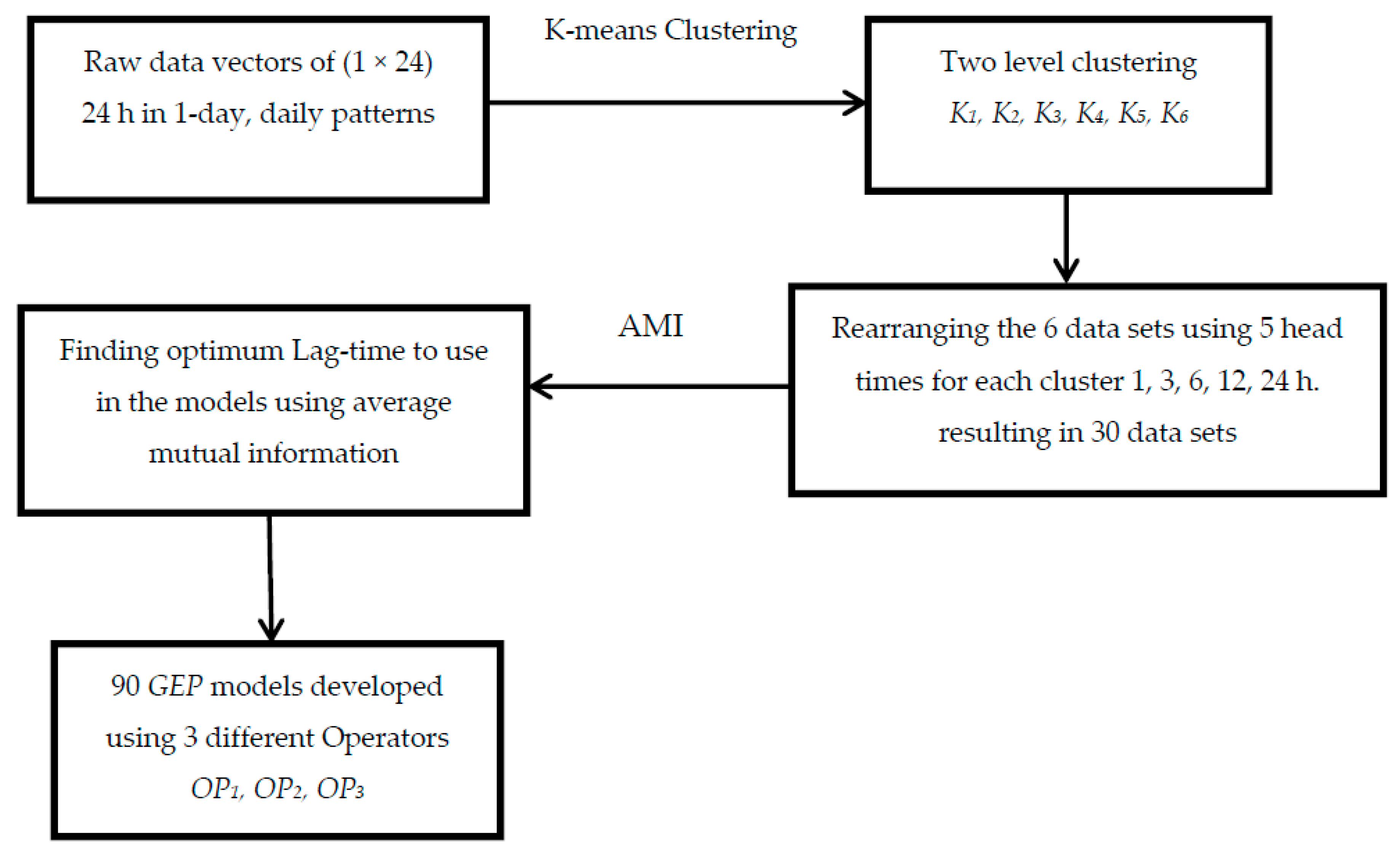
2. Model Development

The input design of the proposed models is based on reaching a broad understanding of the nature of input factors in the data-driven model, the self-interaction of the water demand, and the use of appropriate lag times in demand forecasting models (Figure 1). This is labelled as K_aHT_bOP_c, in which a ∈ [1, 2, 3, 4, 5, 6] number of clusters, b ∈ [1, 2, 3, 4, 5] number of headlines, and c ∈ [1, 2, 3] mathematical operators.

A total of 90 models (6 clusters × 5 head-times × 3 operators) were created. Through a two-stage spherical k-means clustering, data were divided into six different groups. Five different head-times were used to perform a time-scale modeling to obtain the optimum temporal resolution (1, 3, 6, 12, 24 h). Three types of mathematical operators [OP₁, {+, −, ×}; OP₂, {+, −, ×, ×2, ×3}; OP₃, {+, −, ×, ×2, ×3, √, ex, log, ln}] were used in the developing of the GEP models. All of these 90 models were used in partitions of 80% for train and 20% for test sets.

2.1. Unsupervised Learning: K-Means Clusters

The same data were clustered in a study by one of our authors in [33], in which SVM regression is used as forecasting mechanism; therefore, further details on the clustering stage can be found in the related paper. The clustering procedure is briefly summarized here. The time-series used all have the same length: a (1 × 24) vector representing daily water demand. The following picture shows an example of a typical daily water demand pattern selected randomly for illustration.

As Figure 2 shows, the nature of water demand is bound to the temporal shifts, which are due to the habits of consumers in a 24 h time window. Therefore, triangle similarity (also known as cosine similarity) is used in the clustering algorithm, since it can effectively deal with “similarity in time” (temporal alignment of peaks and bursts) [33]. More specifically, two time series are considered similar in time when they vary in a similar way on each time step. Other possible similarities for comparing time series are “similarity in shape”, based on the occurrence of trends at different times or similar sub patterns, and “similarity in change”, which identifies two series as similar according to their variations from time step to time step. As water consumption behaviours can be associated with the recurrent occurrence of peaks and bursts at some hours of the day, the triangle similarity, which is a similarity in time measure, was used to compare and cluster water demand time series. Triangle similarity is the cosine value of the angle between two vectors and is computed as:

$$s(x,y)=\frac{\langle x,y\rangle }{\Vert x\Vert \Vert y\Vert }$$

(1)

It is equal to 1 if x and y have the same orientation, 0 if they are orthogonal, and −1 if they have opposite orientations, independently of their magnitude. Since the components of the urban water demand vectors are not negative, triangle similarity varies in [0; 1].

The main objective of the clustering phase was to group the days in clusters that can consider the seasonality in water consumption behaviours. In order to reach the evidence of this seasonality, a two-level clustering was performed to group the months in the first stage, followed by clustering of the days with the “month clusters”.

The unsupervised learning algorithm used in this paper was k-means, available as “skmeans” among R packages. The following equation shows how the cosine similarity concept is implemented through this algorithm. Calinski-Harabasz and Silhouette proposed methods to measure validity of the numbers of selected clusters [34]. Therefore, they were used to find the optimum number of K in this study. More details on this approach are explained in [33].

$$d\left(x,y\right)=1-s\left(x,y\right)=1-\frac{\langle x,y\rangle }{\Vert x\Vert \Vert y\Vert }$$

(2)

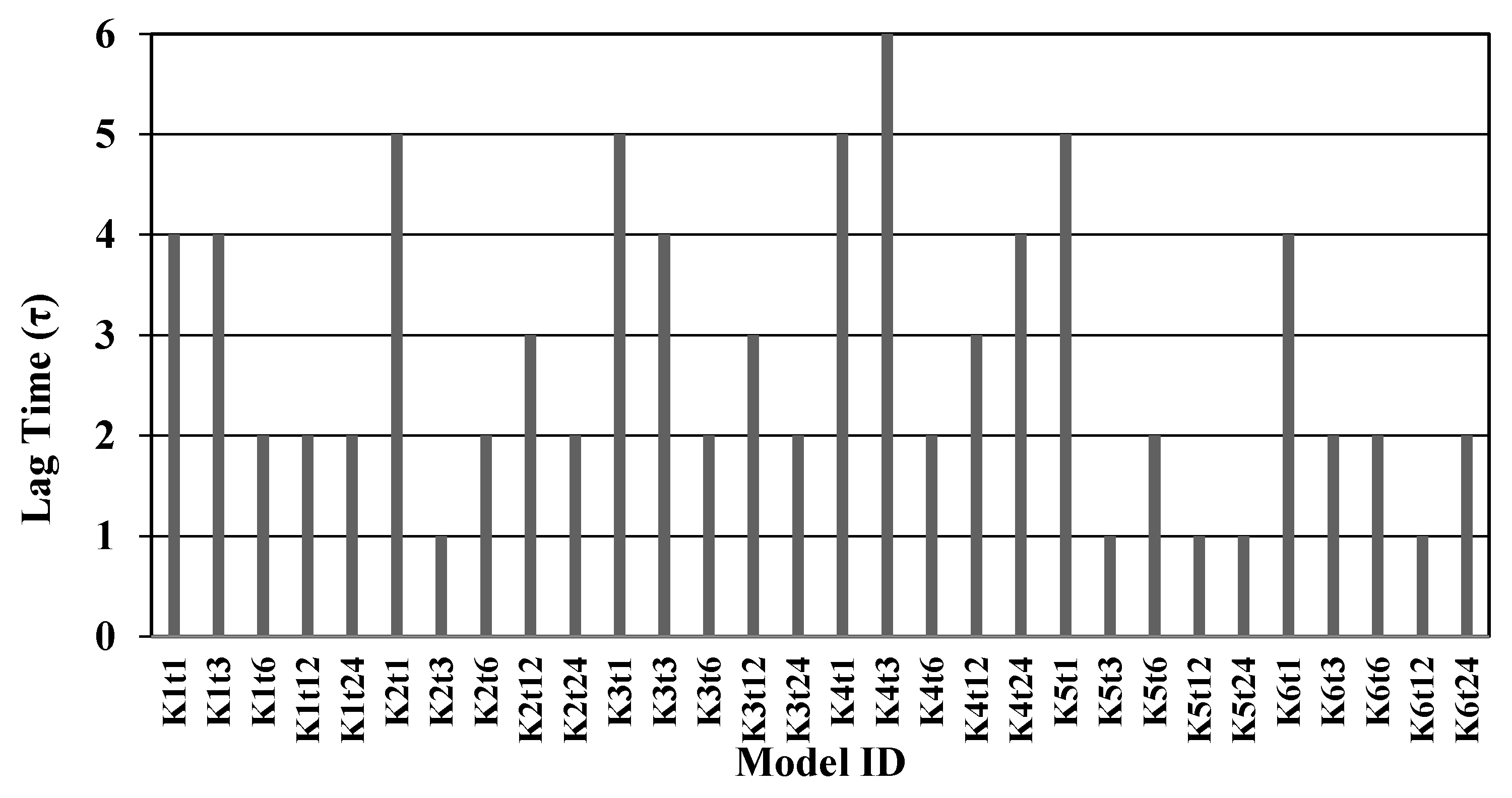
2.2. Average Mutual Information

Performing data-driven models requires selection of an appropriate lag time, as it improves the computational efficiency by adding more valuable information for training, as inputs feeding the GEP models. Traditionally, lag times have been used up to the point where using more lag times would not result in a model’s improvement. Some methods like autocorrelation function (ACF) or correlation integral (CI) methods could bring an educated guess about which lag time should be used in the development of such models [35,36,37]. However, we have used average mutual information (AMI), which does not require large data sets, unlike the ACF and CI methods; it has also been widely used in the field of hydro-informatics in recent years [38]. The following equation is the method for computing AMI for each one of the data sets designed as input variables of the GEP models. It simply uses the joint probability of two successive time series, as well as the marginal probability of them. It should be noted that it is similar to Shannon’s entropy; therefore, it shows less entropy will be in the selection of the optimum lag time based on AMI.

$$I_{\tau }={\displaystyle \sum }_{i=1}^{i=n}P\left(X_i,X_{i+\tau }\right)·{\log }_2\frac{P\left(X_i,X_{i+\tau }\right)}{P\left(X_i\right)·P\left(X_{i+\tau }\right)}$$

(3)

In this equation, the joint probability of two successive time series $P(X(i),X(i+\tau ))$ and the product of their individual marginal probability are used to find the appropriate lag time. This delay can contribute to the maximum valuable information added on $X(i)$ by the successive time series $X(i+\tau )$.

2.3. Gene Expression Programing

GEP’s learning process begins with random generation of chromosomes for the given raw data/population. The generated populations work with two entities: chromosomes and expression trees. Environment selection or the fitness criteria will evaluate which of the offspring solutions can outclass the others. This repetitive process will eventually deliver a good candidate to be selected. In this study, the general settings of the learning/training algorithms were 30 chromosomes, 8 head size, and 3 numbers of genes as suggested. Selection of the head size determined the complexity of each one of the parameters. Each head of the genes was exposed to a variety of arrangements prior to feeding data into the models. Reproduction of the randomly generated populations could reach the superior model with the optimized stopping condition. Figure A1 (Appendix A) shows the expression or tree diagram of the proposed model. As shown, the model was based on 3 genes (sub-expression tree diagrams) linked together by addition function. The number of genes used in a chromosome characterized the different layers/blocks building the whole structure. Using a very big gene could result in more accurate models; however, in this study chromosomes are used in smaller units for simpler computation as a limited number of generations were used. The last part of GEP modelling is selection of stopping condition-function. Root mean square of error (RMSE) was used as fitness function to fit a curve to target values. The stopping condition was 3000 generations for all the runs or models in order to have a fair comparative assessment between all input designs.

Logical sequence of steps in function finding through nonlinear regression of GEP is explained below:

• Creating a random initial population of chromosomes
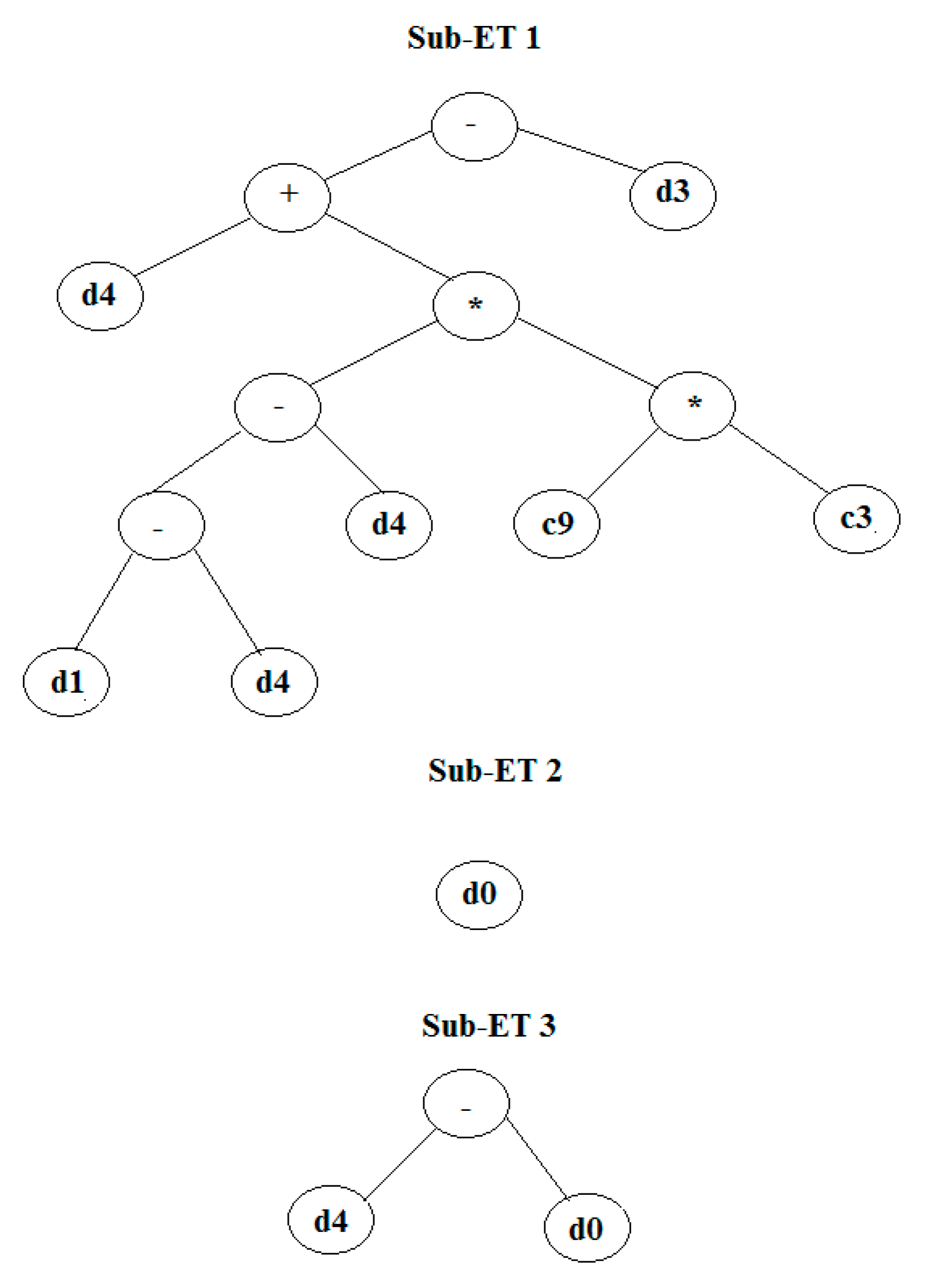
• Expressing chromosomes in a tree diagram with subsets
• Comparing the new offspring solutions based on fitness criteria
• Keeping the best solution, followed by reproduction methods like replication, mutation, recombination, etc.

3. Study Area and Data Collection

The proposed approach mentioned in the previous section was applied to the urban water demand in Milan, Italy, recorded between 1 October 2012 and 30 September 2013. The WDS in Milan serves drinking water to more than 5000 buildings in this city, which serves a population of approximately 1 million people. Other features of this WDS are listed below:

• 149,639 junctions
• 118,950 pipes
• 26 pumping stations
• 501 wells and well pumps
• 33 storage tanks
• 95 booster pumps
• 36,295 valves
• 602 check valves
• Total base demand 7.5 ± 4.2 (m³/s)

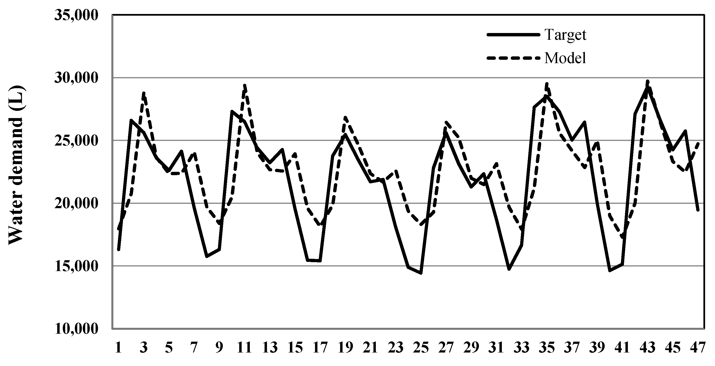
Samples of water demand are recorded through a Supervisory Control and Data Acquisition system (SCADA). Quantity of water pumped into the network by each one of the pumping stations in the city is collected with a sampling rate of 1 sample/min. Collected data are then sent to the centralized SCADA, which sum measures over the different stations to provide the overall water demand of the city. Moreover, SCADA allows for modifying time scale; more specifically, data used in this study were retrieved from SCADA according to an hourly resolution. The multi-scale analysis of the data was performed by scaling the recorded data to head-time bases of hourly, 3 h, 6 h, 12 h, and 24 h. The scaled data were then prearranged into a time-series dataset D = {x₁, x₂, …, x_n} consisting of n vectors, one for each day in the observation period, in which each vector x_i is a set of 24 ordered values for hourly, followed by 8, 4, 2, and 1 for the rest of scaled data, which are under study for the i-th day.

4. Results

The main purpose of clustering in data mining is to illustrate the typical patterns of the trend in consumption of water that are inferred from recurrent peak/burst hours depending only on consumers’ habits. This assignment is done without using any information about the data in the learning process (time of the day or week, and working/non-working days). Since the trend of water consumption follows a specific pattern shown earlier in this paper, “cosine similarity”, known as triangle similarity, was opted for as a similarity index in the clustering process (spherical k-means).

Results of the time-series data clustering (i.e., a two-level clustering approach) allow us to identify 6 typical daily urban water demand patterns (i.e., consumption behaviours), in which the number of clusters was defined according to the best values of the Silhouette and Calinski-Harabasz indices (respectively, 0.74 and 97.87, averaged on the two-level clustering) obtained by varying the possible number of clusters from 2 to 24. More details regarding the detailed results of clustering can be found in [33].

The following Figure 3 shows a calendar with the cluster assignment for every day of the observation period. This kind of visualization makes seasonality and cyclic behaviours more evident. Looking into the 3 clusters of the first stage, one can identify these clusters as (1) Months of November, December, January, February, and March, which correspond to Fall and Winter; (2) Months of April, May, June and September, and October; and (3) July and August, which correspond to the period of largest consumption during summer holidays. The second level of clustering is to target the working/non-working days, which shows how holidays can affect the consumption behaviour of water demand.

Centroids of the 6 prototypes of daily water demand are shown in Figure 4; looking into this figure, one can easily recognize the differences in the peaks of the mornings and evenings that differentiate these 6 clustered prototypes. To be more precise, we can capture a meaningful definition that shows the peak in the mornings of holidays and weekends is always delayed by approximately 1 h compared to that of working days for each period of the year.

Results of the AMI code applied on the rescaled time-series for each head-time under study are shown in Figure 5. In this bar chart, X-axis represents all 30 models (6 clusters × 5 head-times) labelled accordingly. Y-axis is the computed AMI value, which is discussed earlier in this paper through equation 2. These values were used to define the data-driven GEP models in this study. It is important to note that the AMI values make sense in that they are always at their maximum value when the head-time is 1 h, except for K₄, in which the maximum is in head-time 3. This exception is due to the fact that the pattern of consumer behaviours shifts temporally. Moreover, more data is acquired when time-scale is on an hourly basis.

Table 1. Performance indices averaged clusters: (a) MAE, (b) RMSE, (c) R², and (d) MAPE %.

(a). MAE * (Mean ± Standard Deviation)
Operator	Head Time = 1	Head Time = 3	Head Time = 6	Head Time = 12	Head Time = 24
GEP-operator_1	0.2409 ± 0.0388	0.7497 ± 0.4449	0.5943 ± 0.3548	0.5399 ± 0.2932	0.6163 ± 0.3039
GEP-operator_2	0.2319 ± 0.0391	0.7448 ± 0.3885	0.4386 ± 0.1096	0.5061 ± 0.1660	0.6242 ± 0.3952
GEP-operator_3	0.2387 ± 0.0444	0.6031 ± 0.2228	0.4854 ± 0.2857	0.5276 ± 0.2211	0.6433 ± 0.3808
(b). RMSE * (Mean ± Standard Deviation)
Operator	Head Time = 1	Head Time = 3	Head Time = 6	Head Time = 12	Head Time = 24
GEP-operator_1	0.3087 ± 0.0563	0.7861 ± 0.3763	0.7731 ± 0.5048	0.6896 ± 0.3230	0.8272 ± 0.5226
GEP-operator_2	0.3048 ± 0.0632	0.8595 ± 0.3398	0.5274 ± 0.1483	0.6215 ± 0.2052	0.8401 ± 0.5591
GEP-operator_3	0.3116 ± 0.0842	0.7627 ± 0.3338	0.6104 ± 0.3661	0.6718 ± 0.2800	0.8149 ± 0.5710
(c). R2 (Mean ± Standard Deviation)
Operator	Head Time = 1	Head Time = 3	Head Time = 6	Head Time = 12	Head Time = 24
GEP-operator_1	0.8900 ± 0.0498	0.4455 ± 0.1681	0.6221 ± 0.2732	0.4227 ± 0.3275	0.3174 ± 0.2151
GEP-operator_2	0.8906 ± 0.0491	0.4332 ± 0.1593	0.6776 ± 0.2314	0.5131 ± 0.2665	0.2229 ± 0.2288
GEP-operator_3	0.8962 ± 0.0569	0.5077 ± 0.2248	0.6551 ± 0.3585	0.4395 ± 0.3204	0.2727 ± 0.2255
(d). MAPE % (Mean ± Standard Deviation)
Operator	Head Time = 1	Head Time = 3	Head Time = 6	Head Time = 12	Head Time = 24
GEP-operator_1	0.900 ± 0.0113	1.2067 ± 0.0080	2.1450 ± 0.0133	1.4267 ± 0.0098	2.0667 ± 0.0106
GEP-operator_2	0.9400 ± 0.0110	1.4367 ±0.0113	2.3933 ± 0.0090	1.5950 ± 0.0012	2.0683 ± 0.0101
GEP-operator_3	0.8850 ± 0.0089	1.2033 ± 0.0115	2.1867 ± 0.0084	1.4667 ± 0.0091	2.0917 ± 0.0010

* MAE and RMSE should have the same unit as the estimated quantity (water demand (L)); however, all values were scaled between 0 and 1 for fair comparative assessment between the head times under study.

shows the performance of GEP models in the testing period separated by the performance indices used (MAE, RMSE, R², and MAPE). It is important to note that these data are averaged on each cluster, since the overall performance is what matters to predictive modelers. However, the detailed results are shown in

Table A1. Detailed performance of all 90 GEP models in both testing and training periods.

Model ID		Training			Test		Model ID		Training			Test
	MAE	RMSE	R2	MAE	RMSE	R2		MAE	RMSE	R2	MAE	RMSE	R2
K1HT1OP1	0.27	0.36	0.88	0.27	0.33	0.91	K4HT1OP1	0.20	0.29	0.92	0.25	0.35	0.84
K1HT1OP2	0.31	0.42	0.84	0.29	0.38	0.86	K4HT1OP2	0.23	0.32	0.90	0.25	0.36	0.82
K1HT1OP3	0.35	0.52	0.75	0.32	0.48	0.78	K4HT1OP3	0.31	0.41	0.84	0.25	0.31	0.90
K1HT3OP1	0.50	0.64	0.64	0.53	0.40	0.65	K4HT3OP1	0.47	0.55	0.70	1.63	1.48	0.38
K1HT3OP2	0.54	0.68	0.67	0.55	0.72	0.62	K4HT3OP2	0.61	0.73	0.49	1.52	1.53	0.32
K1HT3OP3	0.41	0.51	0.74	0.44	0.52	0.75	K4HT3OP3	0.46	0.56	0.69	1.01	1.41	0.24
K1HT6OP1	0.23	0.30	0.91	0.29	0.36	0.89	K4HT6OP1	0.42	0.49	0.76	1.28	1.75	0.13
K1HT6OP2	0.32	0.40	0.84	0.28	0.33	0.91	K4HT6OP2	0.38	0.46	0.81	0.58	0.76	0.28
K1HT6OP3	0.17	0.23	0.95	0.22	0.28	0.93	K4HT6OP3	0.27	0.35	0.88	1.01	1.28	0.07
K1HT12OP1	0.30	0.42	0.82	0.22	0.33	0.88	K4HT12OP1	0.30	0.44	0.80	1.02	1.18	0.09
K1HT12OP2	0.34	0.49	0.77	0.29	0.38	0.84	K4HT12OP2	0.35	0.48	0.76	0.56	0.62	0.55
K1HT12OP3	0.31	0.45	0.79	0.28	0.37	0.84	K4HT12OP3	0.35	0.50	0.75	0.83	1.03	0.15
K1HT24OP1	0.54	0.73	0.47	0.55	0.66	0.38	K4HT24OP1	0.40	0.52	0.72	1.12	1.82	0.26
K1HT24OP2	0.51	0.72	0.48	0.54	0.66	0.25	K4HT24OP2	0.41	0.48	0.78	1.35	1.88	0.14
K1HT24OP3	0.56	0.75	0.43	0.71	0.54	0.11	K4HT24OP3	0.36	0.44	0.80	1.30	1.88	0.27
K2HT1OP1	0.20	0.29	0.93	0.22	0.27	0.94	K5HT1OP1	0.28	0.35	0.89	0.23	0.28	0.90
K2HT1OP2	0.18	0.27	0.93	0.19	0.24	0.95	K5HT1OP2	0.24	0.31	0.91	0.20	0.24	0.92
K2HT1OP3	0.22	0.30	0.91	0.22	0.28	0.93	K5HT1OP3	0.22	0.30	0.92	0.22	0.28	0.92
K2HT3OP1	0.70	0.82	0.32	0.77	0.87	0.30	K5HT3OP1	0.71	0.83	0.30	0.62	0.74	0.25
K2HT3OP2	0.69	0.81	0.34	0.74	0.86	0.33	K5HT3OP2	0.71	0.84	0.32	0.63	0.75	0.26
K2HT3OP3	0.63	0.75	0.43	0.67	0.79	0.43	K5HT3OP3	0.71	0.83	0.30	0.62	0.73	0.27
K2HT6OP1	0.43	0.51	0.74	0.45	0.55	0.72	K5HT6OP1	0.49	0.60	0.64	0.52	0.59	0.63
K2HT6OP2	0.34	0.45	0.80	0.35	0.43	0.87	K5HT6OP2	0.45	0.55	0.71	0.44	0.51	0.66
K2HT6OP3	0.36	0.45	0.80	0.34	0.42	0.89	K5HT6OP3	0.34	0.48	0.77	0.34	0.46	0.80
K2HT12OP1	0.40	0.53	0.72	0.34	0.45	0.78	K5HT12OP1	0.70	0.78	0.35	0.64	0.80	0.35
K2HT12OP2	0.43	0.56	0.69	0.45	0.54	0.80	K5HT12OP2	0.70	0.78	0.35	0.64	0.80	0.35
K2HT12OP3	0.45	0.59	0.65	0.40	0.46	0.81	K5HT12OP3	0.68	0.72	0.38	0.58	0.75	0.44
K2HT24OP1	0.57	0.82	0.34	0.50	0.63	0.13	K5HT24OP1	0.63	0.81	0.33	0.81	0.95	0.08
K2HT24OP2	0.58	0.80	0.34	0.41	0.52	0.12	K5HT24OP2	0.64	0.83	0.29	0.78	1.05	0.06
K2HT24OP3	0.58	0.80	0.34	0.41	0.52	0.13	K5HT24OP3	0.67	0.79	0.36	0.80	1.05	0.08
K3HT1OP1	0.19	0.24	0.95	0.18	0.23	0.93	K6HT1OP1	0.33	0.43	0.81	0.30	0.38	0.82
K3HT1OP2	0.21	0.28	0.93	0.21	0.27	0.92	K6HT1OP2	0.29	0.39	0.85	0.25	0.34	0.86
K3HT1OP3	0.19	0.25	0.94	0.20	0.25	0.93	K6HT1OP3	0.26	0.36	0.88	0.22	0.28	0.91
K3HT3OP1	0.60	0.73	0.46	0.55	0.67	0.45	K6HT3OP1	0.42	0.57	0.67	0.41	0.55	0.64
K3HT3OP2	0.60	0.75	0.46	0.56	0.69	0.45	K6HT3OP2	0.45	0.58	0.70	0.48	0.60	0.63
K3HT3OP3	0.47	0.56	0.74	0.43	0.53	0.73	K6HT3OP3	0.45	0.59	0.66	0.46	0.59	0.61
K3HT6OP1	0.71	0.87	0.33	0.62	0.87	0.52	K6HT6OP1	0.33	0.43	0.81	0.40	0.52	0.84
K3HT6OP2	0.58	0.69	0.54	0.50	0.62	0.58	K6HT6OP2	0.45	0.55	0.70	0.47	0.51	0.77
K3HT6OP3	0.58	0.73	0.50	0.61	0.78	0.35	K6HT6OP3	0.38	0.48	0.79	0.40	0.45	0.89
K3HT12OP1	0.48	0.59	0.65	0.36	0.49	0.24	K6HT12OP1	0.68	0.92	0.14	0.66	0.89	0.19
K3HT12OP2	0.41	0.50	0.75	0.38	0.47	0.37	K6HT12OP2	0.73	0.94	0.12	0.73	0.92	0.17
K3HT12OP3	0.40	0.50	0.75	0.35	0.47	0.27	K6HT12OP3	0.65	0.89	0.22	0.73	0.95	0.12
K3HT24OP1	0.42	0.52	0.73	0.46	0.54	0.37	K6HT24OP1	0.30	0.44	0.80	0.26	0.36	0.68
K3HT24OP2	0.53	0.63	0.63	0.40	0.56	0.10	K6HT24OP2	0.32	0.46	0.78	0.26	0.37	0.67
K3HT24OP3	0.42	0.52	0.72	0.37	0.51	0.37	K6HT24OP3	0.31	0.45	0.80	0.28	0.39	0.67

(Appendix A) for further investigation of these performances. Results showed the hourly-based models could significantly outperform the other sampling rate/frequencies. It was expected that hourly-based models could come out on top, since data-driven methods perform better with larger data sets. It is known that aggregating the data temporally can improve forecasting due to the temporal averaging which reduces the noise; however, since averaging was not the focus of this study, higher head times did not improve the models. Another valid reason is “oversampling”, which can increase the resolution of the data; consequently, there would be a better definition of the trend in the time series. Moreover, it is known that temporal aggregations can lead to loss of valuable information about the primary data process. MAE measures the mean absolute error between prediction and actual values. The GEP operators performed similarly, as MAE values are very close to each other (MAE of 0.2319 ± 0.0391 being the best using 2nd GEP operator Table 1a). The same story was repeated for RMSE, as 2nd GEP operator outperformed other models with RMSE of 0.3048 ± 0.0632 Table 1b. The third GEP operator was the best among all R², with the highest value of 0.8962 ± 0.0569 averaged on clusters. Interestingly, the performance of 6-h head-time models was significantly better than 3-h models. This improved performance might be because the behaviour of consumer’s demand or the temporal shifts of the consumption can be better defined with a frequency of 1 sample per 6 h rather than 3 h. In other words, resolution of the data might be better represented using this time-scale. Moreover, it is known that performance of these models deteriorated with less frequent data for 12 and 24 h due to much smaller data sets within these time-scales. Results showed that the mathematical operations used in GEP operators do not play a very significant role; however, since these data are not linear, the second {+, −, ×, ×2, ×3} and third operators {+, −, ×, ×2, ×3, √, ex, log, ln} consistently outperformed the first one {+, −, ×} in all simulations. MAPE (minimum absolute percentage error) is used just for comparing testing sets, since it provides a relative magnitude in terms of percent values. Like other performances indices, the 1 h head time models could outperform others with a value of 0.8850 ± 0.0089 averaged on clusters.

K₃HT₁OP₁ is further investigated as one of the superior models to show how GEP models could perform when hourly data is acquired. Table A1 (Appendix A) shows K₃HT₁OP₁ is selected with highest values of R², 0.95, and 0.93 for training and testing data set accordingly. A model that is neither over nor under-trained should have similar performances in test and train periods, an important point overlooked by many scholars in our area. On the other hand, MAE and RMSE values were also the lowest compared to other models with 0.19 and 0.24 for training set, followed by 0.18 and 0.23 for testing set. Figure A2 illustrates how close the prediction and actual demand are for this particular model.

5. Conclusions

The prime objective of this paper was to propose a coupled deployment of supervised and unsupervised learning in short-term water demand forecast models. Time-scale modeling of water demand can lead to a comprehensive understanding of the temporal resolution of this complex system, mainly the pattern of consumption. Having access to hourly water consumption is not very common in many developing countries’ WDS; therefore, this approach gives an idea about the magnitude of errors in the comparative assessments between the time-scale models, helping the operators come up with an appropriate data acquisition frequency.

In the proposed two stage approach, spherical k-means clustering was used to organize daily water demand patterns into six different clusters based on the computed Silhouette and Calinski-Harabasz indices. Gene expression programming was further used, as our supervised learning part of the approach, to model these six clusters separately. The measurement of errors in this paper was done using four performance indices on both training and testing data sets. MAE, RMSE, R², and MAPE are the common methods of error measurement in the field of hydro-informatics, and they are widely adopted among researchers.

Results of this study proved GEP should receive more attention in this area due to the highly accurate predictions it can provide while coupled with unsupervised learning algorithms. It is not a black-box model like the majority of the proposed ANN or SVM models; therefore, meaningful self-interactive relations within the input water demand will be provided, as well as a mathematical equation (through nonlinear regression) to be used by operators of WDS (Appendix A, Figure A1 and Python code in Supplementary Materials for detailed equation). The proposed approach could have a profound impact on the operations of water utilities, as well as on managerial decisions. The frequency of the collected data is a major decision that is used to plan for the next hour, week, month, or even year. The seasonality of water demand patterns is not a new thing; however, the two-level clustering provided (in a completely unsupervised and data-driven paradigm) six groups of data that are not usually used in classified data of predictive models in this field. The positive impacts of this approach are a better understanding of how one can utilize the time series of water demand in short-term forecasting through a completely data-driven technique with a fair understanding of how to opt for the suitable temporal resolution, the proper lag time of the feeding inputs to the models, and an equation/function that can help the operators to use a wide range of models based on their desired duration or the time of year.

References

1. Gleick, P.H. The World’s Water Volume 7: The Biennial Report on Freshwater; Island Press: Washington, DC, USA, 2011. [Google Scholar]
2. Mamo, T.G.; Juran, I.; Shahrour, I. Urban water demand forecasting using the stochastic nature of short term historical water demand and supply pattern. J. Water Resour. Hydraul. Eng. 2013, 2, 92–103. [Google Scholar]
3. Ghiassi, M.; Zimbra, D.; Saidane, H. Urban water demand forecasting with a dynamic artificial neural network model. J. Water Resour. Plan. Manag. 2008, 134, 138–146. [Google Scholar] [CrossRef]
4. Cao, L. Data science: A comprehensive overview. ACM Comput. Surv. (CSUR) 2017, 50, 43. [Google Scholar] [CrossRef]
5. Gupta, A.; Mishra, S.; Bokde, N.; Kulat, K. Need of smart water systems in India. Int. J. Appl. Eng. Res. 2016, 11, 2216–2223. [Google Scholar]
6. Bougadis, J.; Adamowski, K.; Diduch, R. Short-term municipal water demand forecasting. Hydrol. Process. 2005, 19, 137–148. [Google Scholar] [CrossRef]
7. Jain, A.; Ormsbee, L.E. Short-term water demand forecast modeling techniques—Conventional methods versus AI. J. Am. Water Works Assoc. 2002, 94, 64–72. [Google Scholar]
8. Adamowski, J.F. Peak daily water demand forecast modeling using artificial neural networks. J. Water Resour. Plan. Manag. 2008, 134, 119–128. [Google Scholar] [CrossRef]
9. Gato, S.; Jayasuriya, N.; Roberts, P. Temperature and rainfall thresholds for base use urban water demand modelling. J. Hydrol. 2007, 337, 364–376. [Google Scholar] [CrossRef]
10. Shabani, S.; Yousefi, P.; Adamowski, J.; Naser, G. Intelligent soft computing models in water demand forecasting. In Water Stress in Plants; InTech: London, UK, 2016. [Google Scholar]
11. Bakker, M.; Van Duist, H.; Van Schagen, K.; Vreeburg, J.; Rietveld, L. Improving the performance of water demand forecasting models by using weather input. Procedia Eng. 2014, 70, 93–102. [Google Scholar] [CrossRef]
12. Maidment, D.; Parzen, E. Monthly water use and its relationship to climatic variables in Texas. Water Resour. Bull. 1984, 19, 409–418. [Google Scholar]
13. Brekke, L.; Larsen, M.D.; Ausburn, M.; Takaichi, L. Suburban water demand modeling using stepwise regression. J. Am. Water Works Assoc. 2002, 94, 65. Available online: https://search.proquest.com/openview/bdbe337b223db024059c1efb7c6028f4/1?pq-origsite=gscholar&cbl=25142 (accessed on 31 July 2017).
14. Polebitski, A.S.; Palmer, R.N.; Waddell, P. Evaluating water demands under climate change and transitions in the urban environment. J. Water Resour. Plan. Manag. 2010, 137, 249–257. [Google Scholar] [CrossRef]
15. Alvisi, S.; Franchini, M.; Marinelli, A. A short-term, pattern-based model for water-demand forecasting. J. Hydroinform. 2007, 9, 39–50. [Google Scholar] [CrossRef]
16. Bakker, M.; Vreeburg, J.H.G.; Schagen, K.M.V.; Rietveld, L.C. A fully adaptive forecasting model for short-term drinking water demand. Environ. Model. Softw. 2013, 48, 141–151. [Google Scholar] [CrossRef]
17. Al-Zahrani, M.A.; Abo-Monasar, A. Urban residential water demand prediction based on artificial neural networks and time series models. Water Resour. Manag. 2015, 29, 3651–3662. [Google Scholar] [CrossRef]
18. Tiwari, M.K.; Adamowski, J. Urban water demand forecasting and uncertainty assessment using ensemble wavelet-bootstrap-neural network models. Water Resour. Res. 2013, 49, 6486–6507. [Google Scholar] [CrossRef]
19. Firat, M.; Yurdusev, M.A.; Turan, M.E. Evaluation of artificial neural network techniques for municipal water consumption modeling. Water Resour. Manag. 2009, 23, 617–632. [Google Scholar] [CrossRef]
20. Tiwari, M.K.; Adamowski, J.F. Medium-term urban water demand forecasting with limited data using an ensemble wavelet–bootstrap machine-learning approach. J. Water Resour. Plan. Manag. 2014, 141. [Google Scholar] [CrossRef]
21. Odan, F.K.; Reis, L.F. Hybrid water demand forecasting model associating artificial neural network with Fourier series. J. Water Resour. Plan. Manag. 2012, 138, 245–256. [Google Scholar] [CrossRef]
22. Huang, L.; Zhang, C.; Peng, Y.; Zhou, H. Application of a combination model based on wavelet transform and KPLS-ARMA for urban annual water demand forecasting. J. Water Resour. Plan. Manag. 2013, 140. [Google Scholar] [CrossRef]
23. Herrera, M.; Torgo, L.; Izquierdo, J.; Pérez-García, R. Predictive models for forecasting hourly urban water demand. J. Hydrol. 2010, 387, 141–150. [Google Scholar] [CrossRef]
24. Shabani, S.; Yousefi, P.; Naser, G. Support Vector Machines in Urban Water Demand Forecasting Using Phase Space Reconstruction. Procedia Eng. 2017, 186, 537–543. [Google Scholar] [CrossRef]
25. Goyal, M.K.; Bharti, B.; Quilty, J.; Adamowski, J.; Pandey, A. Modeling of daily pan evaporation in sub-tropical climates using ANN, LS-SVR, Fuzzy Logic, and ANFIS. Expert Syst. Appl. 2014, 41, 5267–5276. [Google Scholar] [CrossRef]
26. Brentan, B.M.; Luvizotto, E., Jr.; Herrera, M.; Izquierdo, J.; Pérez-García, R. Hybrid regression model for near real-time urban water demand forecasting. J. Comput. Appl. Math. 2017, 309, 532–541. [Google Scholar] [CrossRef]
27. Ferreira, C. What Is Gene Expression Programming? Idea Group Publishing: London, UK, 2008. [Google Scholar]
28. Shiri, J.; Marti, P.; Singh, V.P. Evaluation of gene expression programming approaches for estimating daily evaporation through spatial and temporal data scanning. Hydrol. Process. 2014, 28, 1215–1225. [Google Scholar] [CrossRef]
29. Fernando, A.K.; Shamseldin, A.Y.; Abrahart, R.J. Use of gene expression programming for multimodel combination of rainfall-runoff models. J. Hydrol. Eng. 2011, 17, 975–985. [Google Scholar] [CrossRef]
30. Stull, R. Wet-bulb temperature from relative humidity and air temperature. J. Appl. Meteorol. Climatol. 2011, 50, 2267–2269. [Google Scholar] [CrossRef]
31. Kisi, O.; Shiri, J. Precipitation forecasting using wavelet-genetic programming and wavelet-neuro-fuzzy conjunction models. Water Resour. Manag. 2011, 25, 3135–3152. [Google Scholar] [CrossRef]
32. Fu, T.C. A review on time series data mining. Eng. Appl. Artif. Intell. 2011, 24, 164–181. [Google Scholar] [CrossRef]
33. Candelieri, A. Clustering and Support Vector Regression for Water Demand Forecasting and Anomaly Detection. Water 2017, 9, 224. [Google Scholar] [CrossRef]
34. Arbelaitz, O.; Gurrutxaga, I.; Muguerza, J.; Pérez, J.M.; Perona, I. An extensive comparative study of cluster validity indices. Pattern Recognit. 2013, 46, 243–256. [Google Scholar] [CrossRef]
35. Fraser, A.M.; Swinney, H.L. Independent coordinates for strange attractors from mutual information. Phys. Rev. A 1986, 33, 1134–1140. [Google Scholar] [CrossRef]
36. Holzfuss, J.; Mayer, G. An approach to error-estimation in the application of dimension algorithms. In Dimensions and Entropies in Chaotic Systems; Mayer-Kress, G., Ed.; Springer: New York, NY, USA, 1986; pp. 114–122. [Google Scholar]
37. Hegger, R.; Kantza, B.; Schreiber, T. Practical implementation of nonlinear time series methods: The TISEAN package. Chaos 1999, 9, 413–435. [Google Scholar] [CrossRef] [PubMed]
38. Khatibi, R.; Sivakumar, B.; Ghorbani, M.A.; Kisi, O.; Kocak, K.; Zadeh, D.F. Investigation chaos in river stage and discharge time series. J. Hydrol. 2012, 414–415, 108–117. [Google Scholar] [CrossRef]
Figure 1. Schematic of the proposed approach.
Water 10 00142 g001
Figure 2. An example of time series data representing hourly water consumption in a day (L/h).
Water 10 00142 g002
Figure 3. Cluster assignments over the observation period.
Water 10 00142 g003
Figure 4. The k = 6 typical water demand patterns identified through the two-level clustering procedure. The cluster assignment is the same as the previous Figure 3.
Water 10 00142 g004
Figure 5. Average mutual information for all input designs k1,…,6 clusters t1,3,6,12,24 head times.
Water 10 00142 g005