Variations in Soil Water Content, Infiltration and Potential Recharge at Three Sites in a Mediterranean Mountainous Region of Baja California, Mexico

Abstract

In this research, we examined temporal variations in soil water content (θ), infiltration patterns, and potential recharge at three sites with different mountain block positions in a semiarid Mediterranean climate in Baja California, Mexico: two located on opposing aspects (south- (SFS) and north-facing slopes (NFS)) and one located in a flat valley. At each site, we measured daily θ between 0.1 and 1 m depths from May 2014 to September 2016 in four hydrological seasons: wet season (winter), dry season (summer) and two transition seasons. The temporal evolution of θ and soil water storage (SWS) shows a strong variability that is associated mainly with high precipitation (P) pulses and soil profile depth at hillslope sites. Results shows that during high-intensity P events sites with opposing aspects reveal an increase of θ at the soil–bedrock interface suggesting lateral subsurface fluxes, while vertical soil infiltration decreases noticeably, signifying the production of surface runoff. We found that the dry soil conditions are reset annually at hillslope sites, and water is not available until the next wet season. Potential recharge occurred only in the winter season with P events greater than 50 mm/month at the SFS site and greater than 120 mm/month at the NFS site, indicating that soil depth and lack of vegetation cover play a critical role in the transport water towards the soil–bedrock interface. We also calculate that, on average, around 9.5% (~34.5 mm) of the accumulated precipitation may contribute to the recharge of the aquifer at the hillslope sites. Information about θ in a mountain block is essential for describing the dynamics and movement of water into the thin soil profile and its relation to potential groundwater recharge.

1. Introduction

Understanding the dynamics and transport of soil water content (θ) in thin mountain soils is essential for describing infiltration in superficial and deeper soil layers. Evaluation of the spatial and temporal distribution of θ is also crucial for assessing how recharge might vary with different locations in a mountain block [1,2]. Significant variations in θ depend on climatic forcing [3,4,5,6], soil properties, topography and vegetation [5,7,8,9]. Each of these factors can influence θ over multiple spatiotemporal scales [10] with substantial variations observed with soil depth [11,12,13]. For instance, θ in different soil layers is influenced by the productivity of terrestrial plants with varying rooting depths [14,15,16].

Precipitation pulses are a first-order control on the seasonal variation of θ during the hydrological year, in particular for semiarid regions characterized by long periods of no rainfall [9,17,18]. In semiarid Mediterranean climate systems, the seasonality of precipitation (P) leads to high water availability in the winter season when potential evapotranspiration is low [19]. Winter precipitation influences diffuse recharge processes through vertical infiltration occurring in the soil profile (e.g., [20,21,22,23]). In mountain systems within these settings, soil thickness is generally shallow leading to the potential for rapid flow into fractures that underlie the soil [24]. As a result, the shallow monitoring of θ and its spatiotemporal variability in response to P should yield inferences on potential recharge in mountain block systems.

Mountain block systems often have spatial variations in vegetation mediated by topographic position. For instance, plant distributions in mid-latitude regions exhibit changes between pole-facing slopes and equator-facing slopes (in the northern hemisphere, north (NFS) and south (SFS) facing slopes), and it is recognized as a global phenomenon [25,26,27,28]. This aspect of control is derived from increased exposure to solar radiation on the equator-facing slope and the consequences on the soil water content through evaporation and transpiration [26,29,30,31,32]. Spatial patterns in vegetation also have consequences on the spatiotemporal distributions of θ [25,26] that might affect the potential for recharge in mountain systems on slopes with opposing aspects and soil water storage (SWS). Furthermore, soil-vegetation-terrain feedback processes occur on opposing slopes that alter soil properties and the hillslope form [25], which in turn influence water movement and the distribution of soil water content.

In this research, we analyzed the spatiotemporal variation of θ at different depths to answer the following questions: how do soil depth, aspect, and precipitation magnitude control soil water content and infiltration in semiarid Mediterranean mountain systems? What are the possible implications of these terrain and climatic characteristics on potential recharge? To address these questions, we established soil water monitoring systems (for depths from 0.1 to 1 m) at three sites with different ecological and terrain characteristics: two sites on opposing aspects and one in an intervening flat area. We compared the soil water content during four hydrological seasons and inferences were made with respect to vertical infiltration, SWS, and potential recharge. The comparison across sites was intended to yield information on potential recharge, which is important for quantifying available water resources in downstream valley areas.

2. Methods

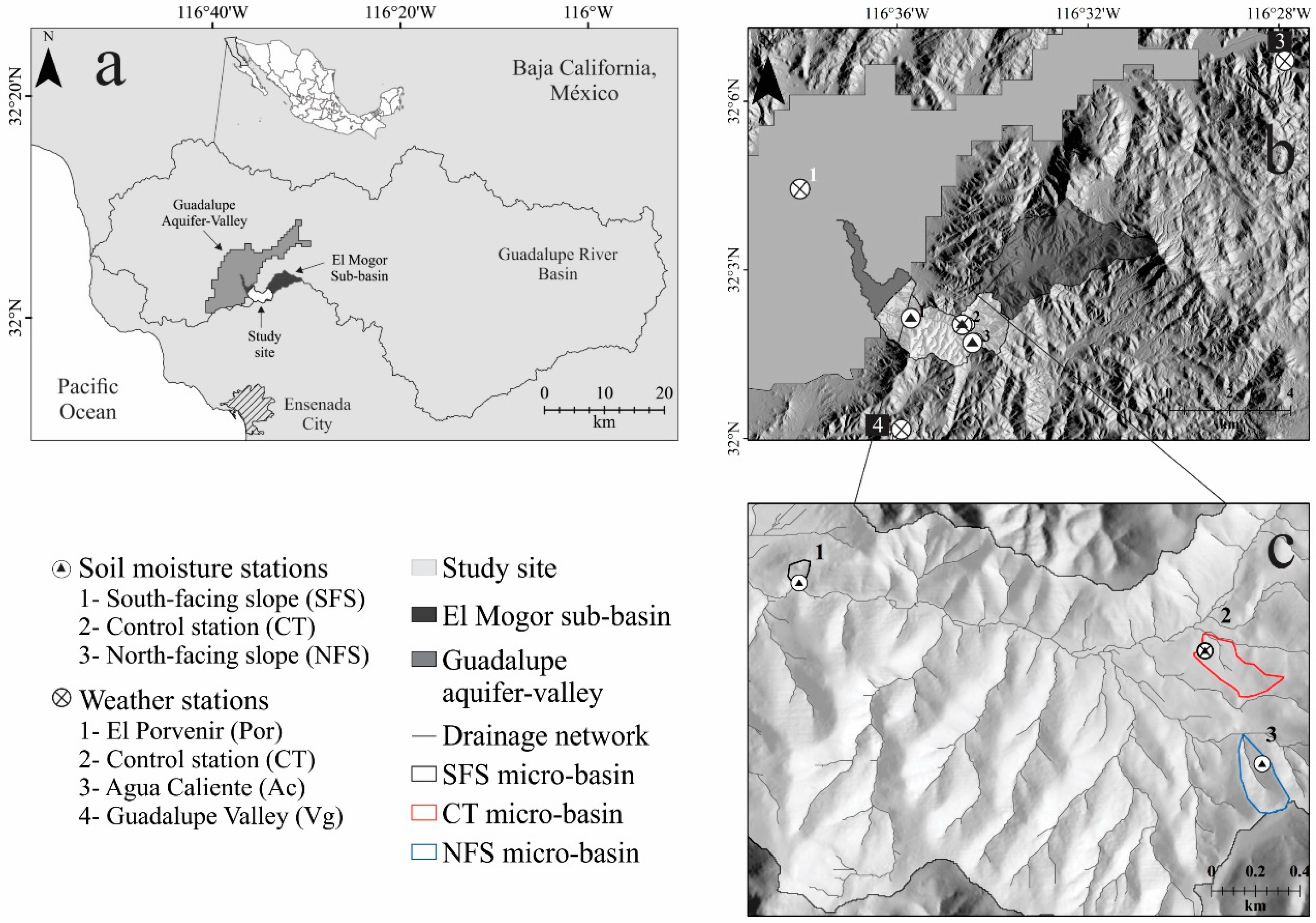
2.1. Geographic and Climatic Setting

This study was conducted in the sub-basin “El Mogor” (~1929 ha) located 26 km northeast of Ensenada, Baja California, Mexico (Figure 1a). The watershed drains towards the west into the Guadalupe Valley, known for its agricultural activities including wine production [33,34]. We selected the central portion of the sub-basin as our study site (~694 ha) because of the access and security provided by a private landowner. There are several research papers that provide detailed descriptions about the characteristics of the study site [19,35,36].

The region has a semiarid Mediterranean-type climate [37]. We calculate an average annual temperature of 17.2 °C and average annual precipitation of 330 mm, using historically recorded data from El Porvenir weather station (1991–2016) from the Mexican National Water Commission, located 7 km northwest of the site at an elevation of 320 masl (Figure 1b). Within El Mogor, climatic data were recorded from a weather station installed at a control site at 430 masl (CT station; Figure 1c) over four hydrologic years (2012–2013 to 2015–2016). During the study period, a below-average P of 228 mm per year was recorded, while the annual temperature of 17.2 °C was the same as at El Porvenir.

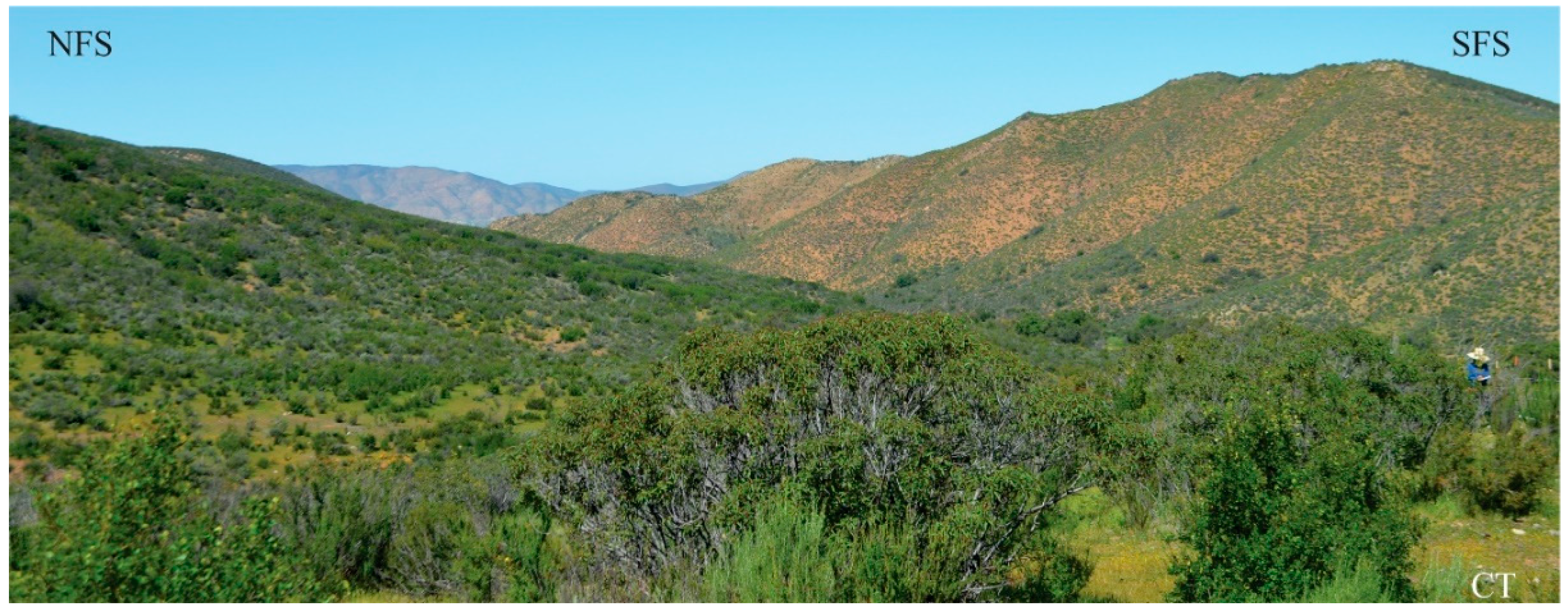
2.2. Site Description

Chaparral shrubs cover entirely the study site of the sub-basin and the micro-basins under analysis (~10.3 ha). The natural ecosystem was clearly structured by variations in aspect. Figure 2 shows the vegetation differences between pole-facing and equator-facing slopes in our study site. In this case, a more xeric vegetation exists on the equator-facing slopes, while a more mesic vegetation prevails in the pole-facing slopes. The northern micro-basin (0.82 ha) is composed exclusively of SFS, which leads to sparse and xeric vegetation, small shrubs (less than 1 m) and the absence of grasses even in wet season. Dominant plant species are Eriogonum fasciculatum (California buckwheat) and Bahiopsis laciniata (San Diego County viguiera) [32,35]. In contrast, the southern micro-basin (4.53 ha) is dominated by NFS which cover about 80% of the area while the 20% remaining includes west-facing slopes. Here, vegetation is denser (more mesic), small and medium shrubs prevail, and herbaceous plants appear at ground level in wet season. Higher woody plant diversity is present, including Eriogonum fasciculatum, Fraxinus parryi (Chaparral ash), Condea emoryi (Desert lavender), Malosma laurina (Laurel sumac), Salvia apiana (White sage), Adenostoma fasciculatum (Chamise), Artemisia californica (California sagebrush), Bahiopsis laciniata and Baccharis salicifolia (Mule fat) [35]. The CT micro-basin (4.97 ha) is located in the transition of the southern and northern micro-basins, over a small inter-mountainous valley. At CT, vegetation is similar to the NFS in terms of cover and diversity of plant species. In addition, grasses are present in the wet season and there is a presence of small patches of trees.

Throughout the sites, the soil type is classified as Haplic Phaeozem. Plant roots are evident in the shallow topsoil layer at the three sites. Deeper, soil horizons where poorly differentiated until reaching bedrock on the hillslopes sites. Total soil depth is shallower at SFS site (~0.4 m) than at the NFS site (~1 m), because SFS is more affected by fluvial erosion processes due to lack of vegetation cover. Residual parent material is formed by fractured siliceous rocks (granite, granodiorite and tonalite) [38]. It should be mentioned that the soil depth at the CT site was measured with a drilling machine and reach approximately 7.5 m depth.

2.3. Terrain Attributes

We employed a digital terrain model with a spatial resolution of 5 m derived from an aerial Light Detection and Ranging (LiDAR) survey [39] to calculate terrain characteristics for the study site. We calculated a set of topographic indices to analyze the influence of flow attributes (hypsometry, slope aspect, curvature), nonlocal morphometric variables (catchment area) and combined morphometric variables (topographic wetness index, [40]) on each micro-basin and our observation sites.

2.4. Site Instrumentation and Study Period

Soil moisture was measured with multi-sensor profilers PR2 (Delta-T Devices), with data loggers DL6 or GP2 (Delta-T Devices), recorded every 30 min to obtain θ in m³/m³. A PR2/4 profile probe with 4 sensors at different depth intervals was used at the SFS site (0.1, 0.2, 0.3 and 0.4 m), while at the CT and NFS sites a PR2/6 profile probe with 6 sensors at different depth intervals were installed (0.1, 0.2, 0.3, 0.4, 0.6 and 1 m). Detailed descriptions of sensor operation have been reported in several studies [41,42,43] and in the sensor operation manual [44]. Installation of the sensors was carried out using a drill bit to place an access tube for the multi-sensor probes. This procedure preserved the natural properties of the soil profile and allowed estimating soil thickness (~0.4 m at SFS and ~1 m at NFS). In addition, a Davis weather station was installed at the CT site to record atmospheric conditions (P and temperature) at 30-min intervals. P was measured with a calibrated precipitation gauge. Datasets were analyzed by event, month and hydrological seasons: wet season (WS; December–March), dry season (DS; June–September) and two transitional seasons (TS1 from wet to dry season; April–May; and TS2 from dry to wet season; October–November). The study period began in the middle of TS1 2014 (TS1-14; May) at the SFS and CT sites, while at the NFS site, data collection began at the end of WS 2015 (WS-15; March). Thus, data availability was ~2.3 years at SFS and CT, while ~1.6 years were available at NFS.

2.5. Soil Texture Analysis and Sensor Calibration

For each of the three sites, soil sampling was performed and analyzed to establish textural characteristics and hydraulic properties of each soil layer with hydrometer and sieve analyses (

Table 1. Soil properties for each site by depth. ρ_b (dry bulk density), µ (soil porosity), percentages of sand, silt and clay and soil texture classification.

Site	Depth (m)	ρb (g/cm3)	µ (%)	Sand (%)	Silt (%)	Clay (%)	Texture
SFS	0.1	1.51	43	89	10	1	fine sand
	0.2	1.56	41	89	10	1	fine sand
	0.3	1.56	41	90	9	1	fine sand
	0.4	1.71	36	89	10	1	fine sand
CT	0.1	1.51	43	84	14	2	loamy fine sand
	0.2	1.61	39	85	13	2	loamy fine sand
	0.3	1.56	41	85	13	2	loamy fine sand
	0.4	1.56	41	83	14	3	loamy fine sand
	0.6	1.71	36	87	11	2	fine sand
	1	1.52	43	64	2	34	sandy clay loam
NFS	0.1	1.46	45	85	13	2	loamy fine sand
	0.2	1.41	47	91	7	2	fine sand
	0.3	1.36	49	92	6	2	fine sand
	0.4	1.51	43	94	5	1	fine sand
	0.6	1.61	39	93	6	1	fine sand
	1	1.56	41	95	4	1	fine sand

). Hillslope locations (SFS and NFS) had sand fractions ranging from 85–95%, while CT was only 64–87% in terms of sand fraction (Table 1). In the three soil profiles (0.4 m at SFS; 1 m at NFS; 1 m at CT), the sand fraction was the most dominant, with the remaining soil composed of fine sediments (silt and clay) with a lower percentage of clays (1–1.5% in both sites) (Table 1). Overall soil textural characteristics and relative fractions are consistent in each depth-layer except for the deepest layer at the CT site, composed with 34% of clay fraction (Table 1).

To calibrate the multi-sensors readings, we followed the procedure described in [44] whose methodology is briefly described below. The purpose of calibration is to generate two coefficients (when the soil is moist and when it is dry), which can be used in a linear equation to convert voltage readings into soil moisture from the dielectric properties of the soil (√ε). We collected undisturbed soil samples for each depth-layer (16 samples in total) and measured the field voltage using an HH2 moisture meter and an ML3 sensor from Delta-T Devices. Then, we placed each sample inside of a metallic cylinder (volume~300 cm³) and transported these to a laboratory where wet and dry weights were obtained before and after drying at 105 °C for ~72 h. The output voltage was then measured for dry conditions to obtain both calibration coefficients. To verify the calibration, we related the dielectric soil measurements (√ε) to the sixteen volumetric soil water content samples. The PR2 sensors quoted an error of ~±0.05 m³/m³ or less with a soil-specific calibration.

2.6. Soil Moisture Analyses

We analyzed the temporal variation of θ in terms of SWS in the soil profile at each site during the study period and for the defined seasons. We performed a numerical integration to calculated SWS_ij for site i on day j as:

$$SW{S}_{ij}=1000\ast \left\{\frac{b-a}{c}\ast \left[{\theta }_{ij\left(a\right)}+\cdots +{\theta }_{ij\left(b\right)}\right]\ast d\right\}$$

(1)

where the 1000 is a conversion factor from m to mm, the subscripts indicate the depth of the measurement (θ in m³/m³), a denoting the sensor upper bound, b represents the sensor lowest bound and c is the total length of the sensor rod and d is the length of each profile sensor (0.1 m). We standardized the SWS values by carrying out a transformation:

$$Z_{ij}=\frac{SW{S}_{ij}-{\overline{SWS}}_{ti}}{{\sigma }_{ti}}$$

where $Z_{ij}$ is the standardized variable, subscripts i and j represent the site and day, respectively, ($Z_{ij}$ indicates that at site i conditions were relatively wet if $Z_{ij}$ > 0 or dry if $Z_{ij}$ < 0), the temporal mean (${\overline{SWS}}_{ti})$ and standard deviation (σ_ti) are defined by the total observation days.

Soil moisture analyses at the three sites were related to the precipitation event amount, intensity and monthly accumulation. In total, 14 months were selected with P ranging from 12.6 to 126.6 mm/month. For the remaining months, P pulses were less than 7 mm (29 months). For periods with rainfall, vertical infiltration (Inf in mm) was defined as the total of water amount entering the soil when the wetting front passed the first layer (~0.1 m). Potential recharge (Pr in mm) was then defined as the total of water amount that reached the deepest soil layer in each profile. We calculate both fluxes following [45], where infiltration continues with uniform θ above the wetting front [46] and we estimate infiltration with a modified equation from [46,47], as follows:

$$Inf=\underset{z=0}{\overset{wf}{{\displaystyle \int }}}\left({\theta }_{a\left(z\right)}-{\theta }_{p\left(z\right)}\right)\ast dz\approx 1000\ast \left({\theta }_{a\left(z\right)}-{\theta }_{p\left(z\right)}\right)\ast d$$

(3)

where θ_a is the maximum value of θ recorded after a precipitation pulse (m³/m³), θ_p represents θ measured preceding the pulse (m³/m³), wf is the wetting front depth (m), z symbolizes the terrain surface, 1000 is a conversion factor from m to mm and d is the depth interval (0.1 m). We define the estimation of Inf assuming that θ is uniform at 0.1 m above the depth layer being measured (e.g., at 0.2 m depth, θ is uniform from 0.1 to 0.2 m) and that θ is uniform before the wetting front passage.

3. Results and Discussion

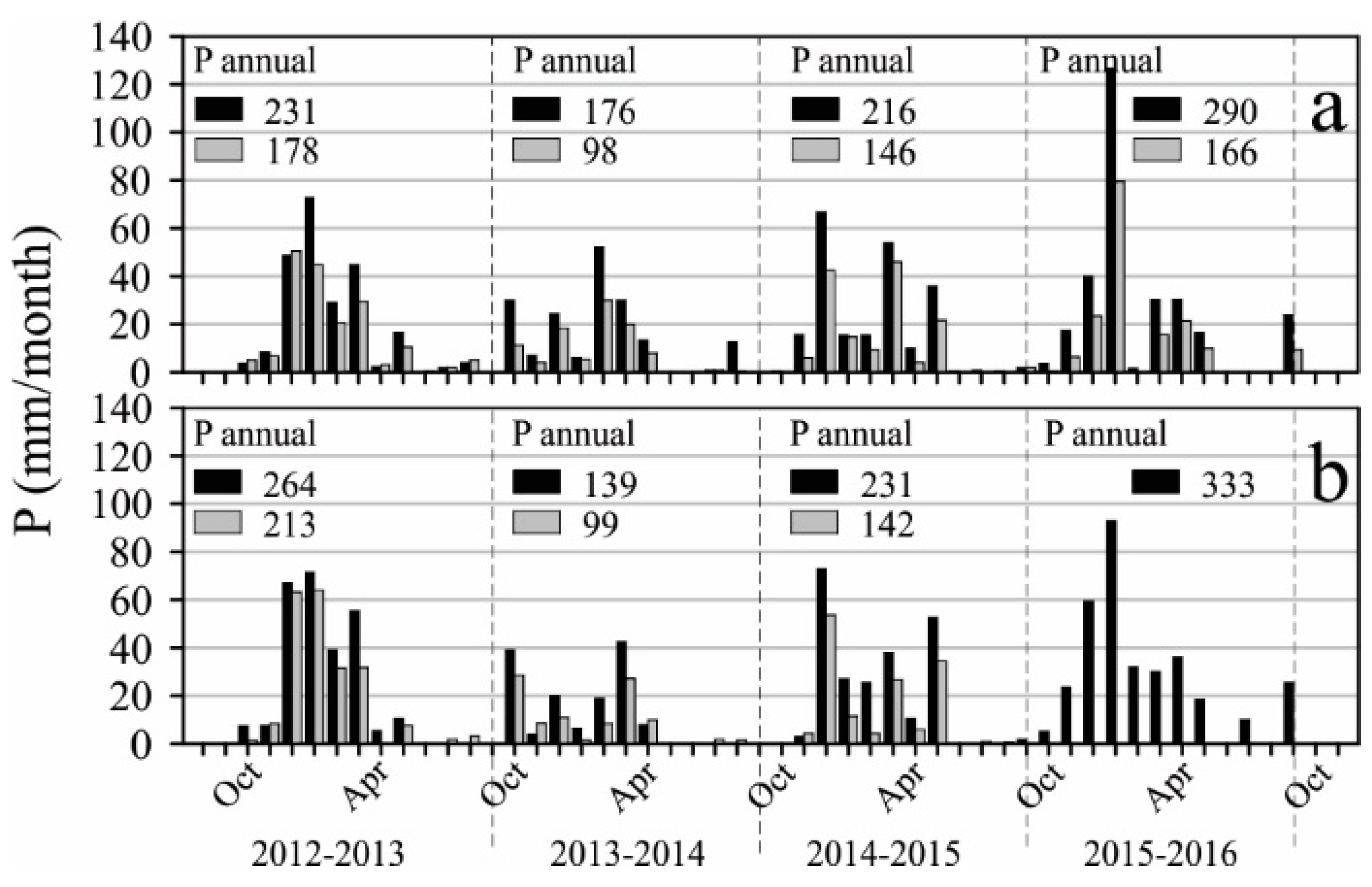
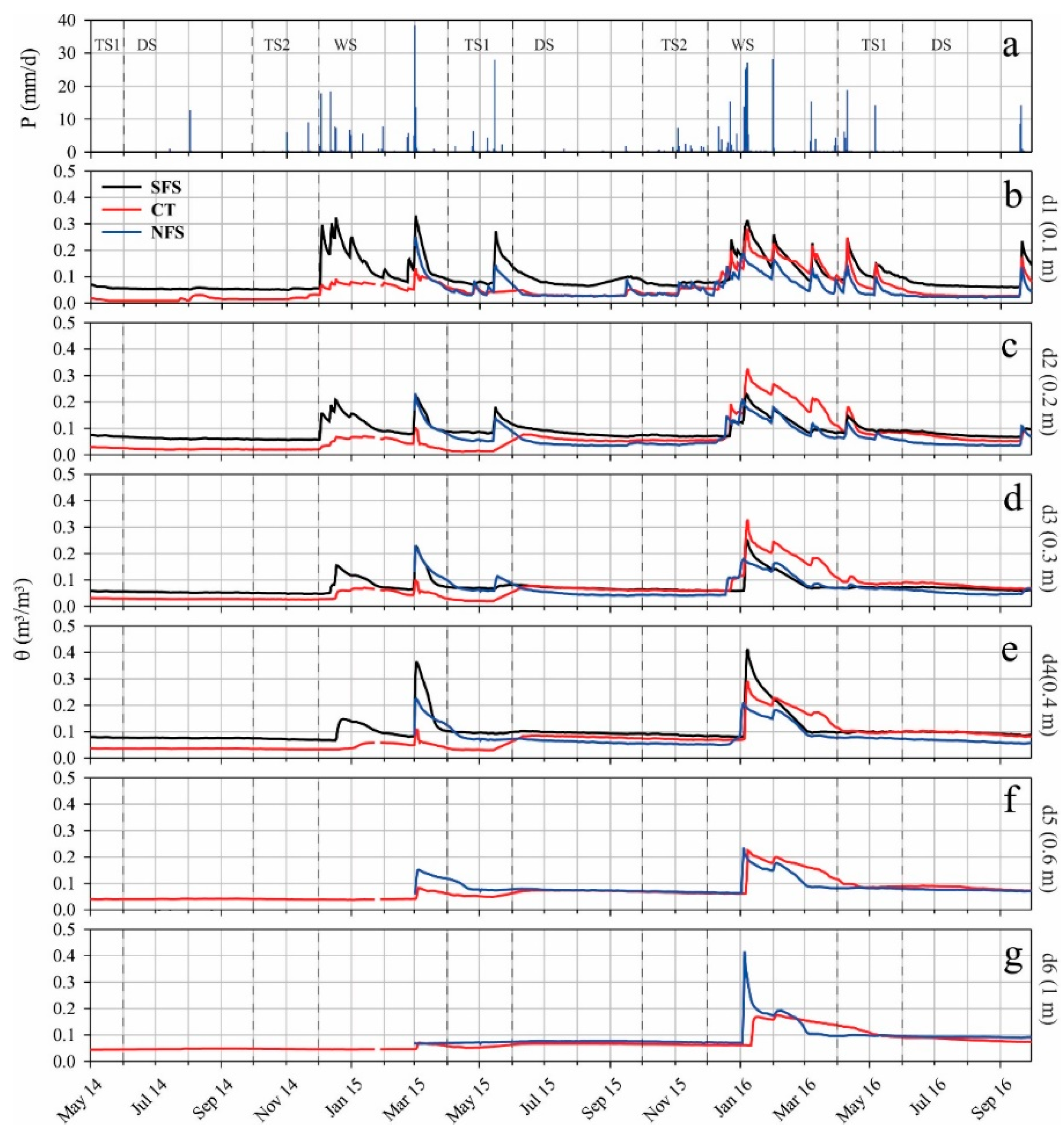
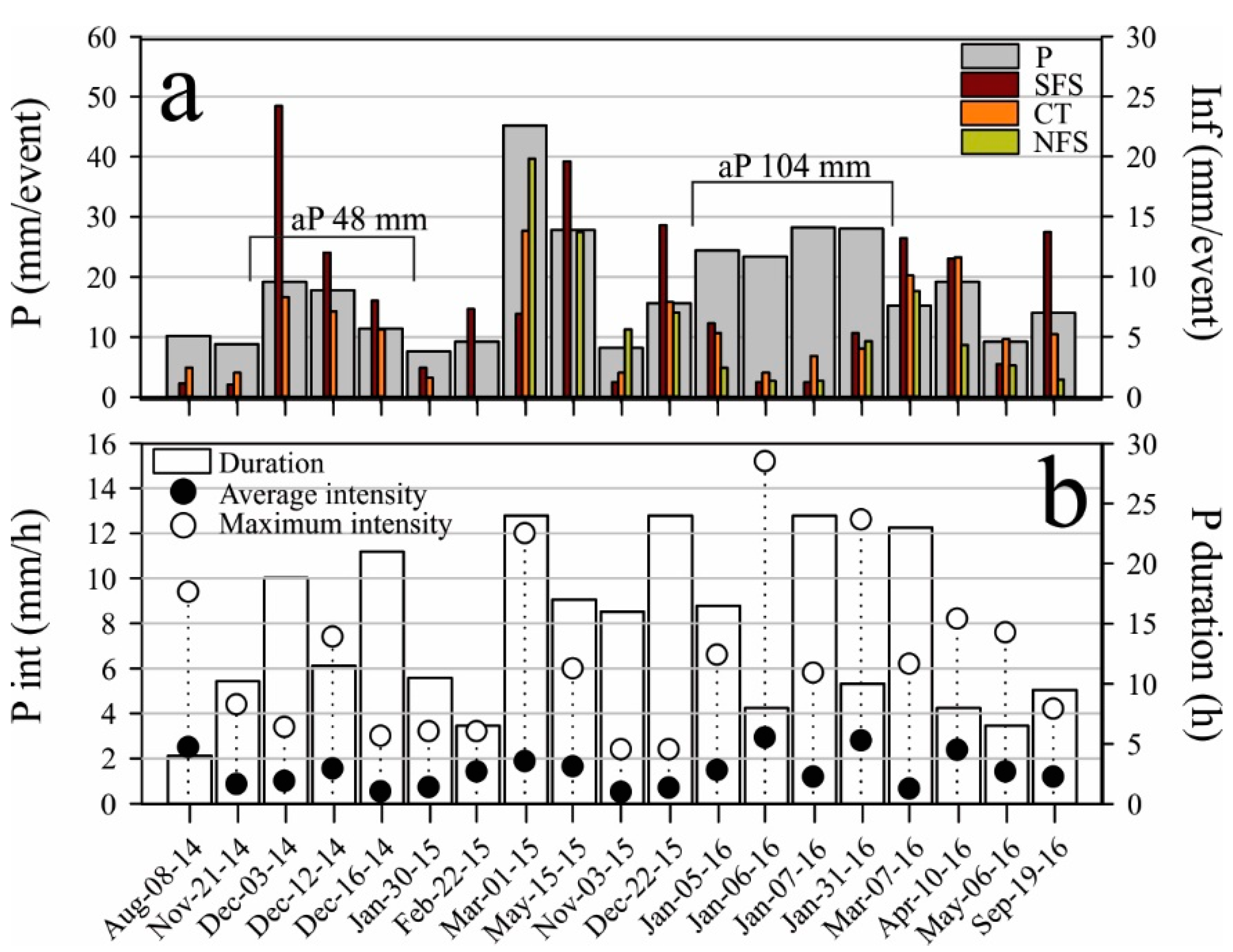
3.1. Precipitation Analyses

Figure 3 shows a monthly and annual P comparison of three surrounding weather stations: El Porvenir (Por), Agua Caliente (Ac), Guadalupe Valley (Vg) and CT in hydrological years 2012 to 2016. Interannual variability was detected except in the dry season (June to September). The total number of precipitation events in the year observed at the CT weather station, varied from 44 to 86 events per year, with a total of 256 days with rainfall from 2012 to 2016 (Figure 3a; black bars). Small precipitation events with P < 2 mm/day were the most representative in the entire period (69% of the total events), while larger events occurred less frequently: P > 2 and <5 mm/day (10%), P > 5 and <10 mm/day (11%), and P > 10 mm/day (10%). The maximum rainfall intensity during the period was 15 mm/h, measured in January 2016. Some days with P > 20 mm/day occurred from January to May.

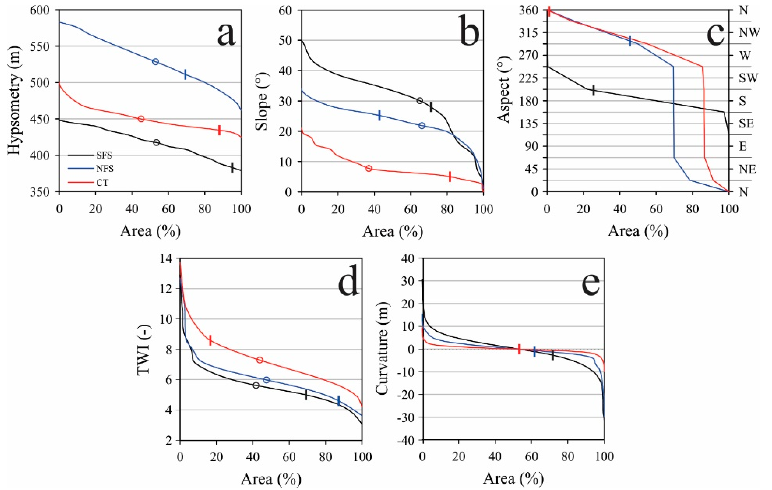
3.2. Terrain Attributes at the Study Sites

We compared the three sites through the distribution of the accumulated area and elevation using hypsometric curves. Convex up profiles of hypsometric curves show active micro-basins at the two hillslope sites (SFS and NFS). Terrain attributes can be used to describe soil erosion and landslide development, as well as to make inferences on soil water and runoff processes [48,49] (Figure 4a,b). The CT site show an intermediate stage basin (Figure 4a,b), wherein a complex interaction of landscape processes is taking place [50,51]. In about 20% of the area, hillslope processes are taking place, while the remaining 80% indicate the development of fluvial processes where mechanisms are different to those described at the hillslope sites. Slope aspect impacts θ due to differences in insolation (SFS tends to have higher radiation than NFS in the northern hemisphere). Slope aspect at SFS basin was clearly south (about 80% area), with SW and SE slopes covering the remaining area. By contrast, the NFS basin had northerly aspects (40% N, 30% NW and 10% NE), with the remaining area characterized with west-facing orientations. At the CT site, NW aspect is dominant (50%), followed by W (20%) and N (20%), with the remaining 10% corresponding to NE facing-slopes (Figure 4c). The topographic wetness index (TWI) is affected by the magnitude of slope and the upslope contributing area. Figure 4d shown the relative trend of TWI in each micro-basin. We observed relatively lower values at hillslope sites than at CT site due to their steeper slope gradients. Curvature (Cur) variations among the micro-basins are shown in Figure 4e. Overall, positive and negative values of curvature are well balanced, although the SFS micro-basin showed more extreme values than NFS. CT micro-basin values tend to be more lineal on the surface (Cur = 0) (Figure 4e). Cur values at SFS, CT and NFS sites show negative values (SFS < NFS < CT), indicating that surface and subsurface flows converge and decelerate, this features indicate that soil moisture content tends to increase at these points, with more potential at the SFS site.

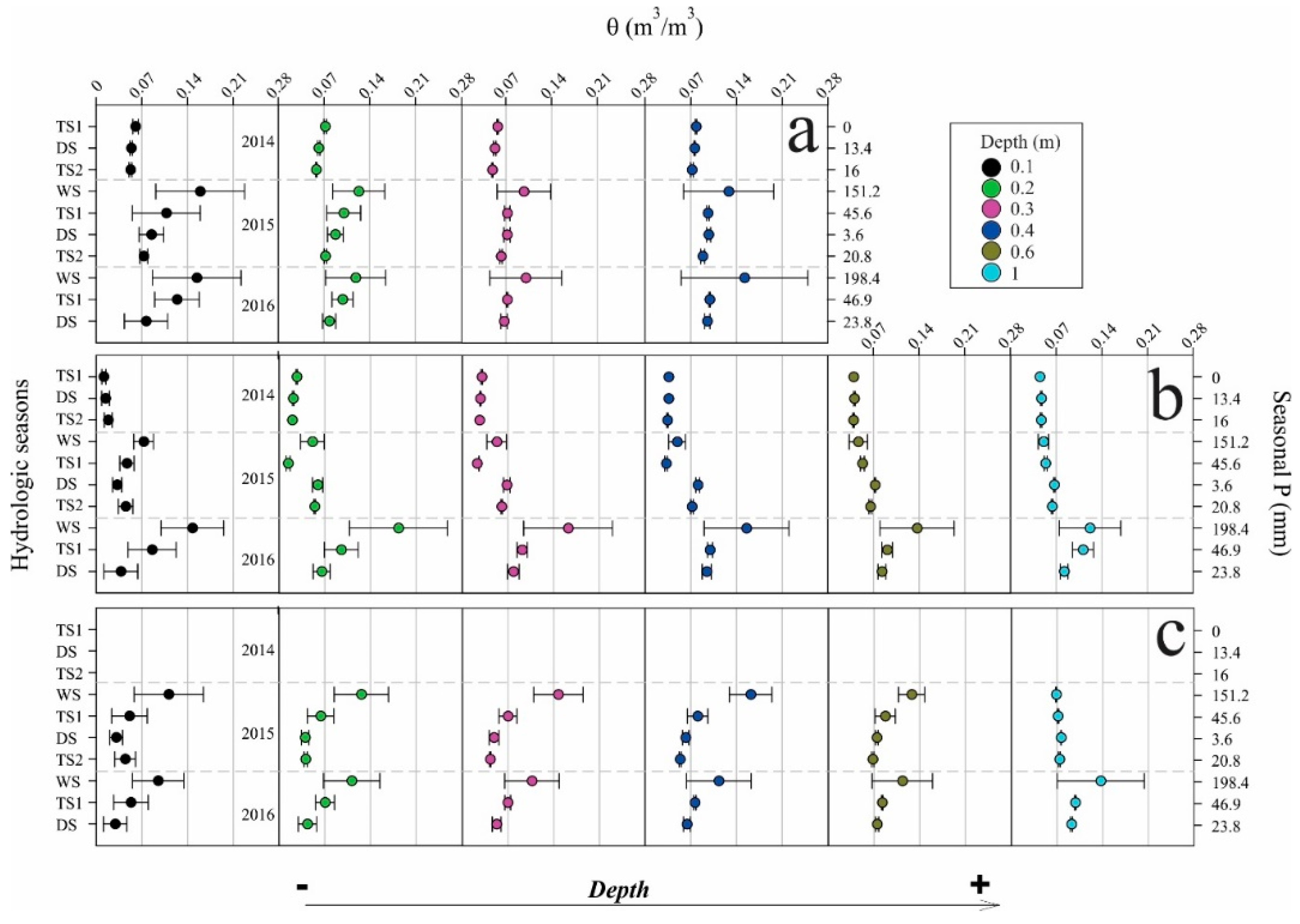
3.3. Temporal Variations of Soil Water Content with Depth

Figure 5 presents daily soil water content for varying depths at the SFS, CT and NFS sites along with daily P during the study period. At the three sites, we found significant differences in daily θ for each soil layer (ANOVA, p < 0.01). High daily θ was observed in winter months (WS) with great precipitation amounts (151.2 and 198.4 mm in WS-15 and WS-16, respectively). Lower θ amounts occurred during transitional seasons (TS1 and TS2) and the summer dry season (DS) with low or no rainfall. TS1 exhibited daily θ superior than TS2 due to more frequent precipitation. Furthermore, daily θ at the monitored depths almost was completely depleted or removed in the dry summer (DS) and in the transition from dry to wet months (TS2) at all sites, indicating a resetting of dry conditions each year. As expected, there was a greater variation of daily θ in the shallower soil layers that were more exposed to precipitation and evaporation. As [12,52,53] showed, for deeper soil layers, the soil water content generally tended to be more stable. Soil moisture observations at hillslope sites show the active response of vertical and lateral θ after a long rainfall pulses of low intensity (e.g., Figure 5; December 2015 at SFS) and long rainfall pulses with medium-high intensity (e.g., Figure 5; March 2015 and January 2016 at SFS and NFS sites; and January 2016 at CT site) respectively. We found at hillslopes sites an atypical increase of θ, near the bottom of the soil profile at the contact with bedrock (e.g., 0.4 m at SFS and 1 m at NFS) (Figure 5e,g). Interestingly, this mechanism was evident at SFS and NFS showing a sharp increase in daily θ that was superior to amounts in shallower (overlying) layers. This could be indicative of gravitational water quickly drained to the soil profile bottom. If bedrock is fractured, this process could promote rapid infiltration towards the mountain block aquifer from that point. However, it could be also indicating a lateral flow from uphill locations transported along the soil-granite bedrock interface, this mechanism has not been documented frequently in opposing slope aspects with varying plant species. For instance, Penna et al. [54] showed the opposite trend, that daily θ on hillslopes decreases with depth up to 20 cm. Gutiérrez-Jurado et al. [55] also showed evidence of lateral water fluxes in different aspect hillslopes after a large storm, but did not attribute this to the effect of the soil–bedrock interface in promoting subsurface transport.

Figure 6 summarizes the temporal dynamics of θ through the mean and standard deviation for each hydrological season and depth. Shallower soil depths had more variable θ across each season, while seasonal variations decreased with soil depth, as noted in other studies (e.g., [16,56]). The decrease and variability in θ at each layer was primarily caused by climatic factors (upper layers) and the uptake of soil water by roots [57] especially in the dry and intermediate seasons, while the larger variation observed in wet seasons is due to lateral flow. For seasons with more cumulative precipitation, the infiltration front reached deeper soil layers. For instance, WS 2016 (P = 198.4 mm) exhibited increased θ throughout the soil profile at all sites. Interestingly, the average seasonal θ during WS 2016 tended to increase with soil depth, reaching maximum values at 0.4 m (SFS), 0.2 m (CT) and 1 m (NFS), with large temporal variations (Figure 6, bars) occurring within the season as well. As noted previously, the high and variable amounts of soil water at depth was an indication of rapid lateral transport at the soil–bedrock interface. Since the overlying shallow layers did not exhibit the same behavior, the soil water during wet seasons is likely to derive from uphill locations. This suggests that steep areas with shallow soils in mountain block systems transport water laterally on the soil–bedrock surface [58,59,60] thus effectively bypassing the shallower soils which are more exposed to evapotranspiration.

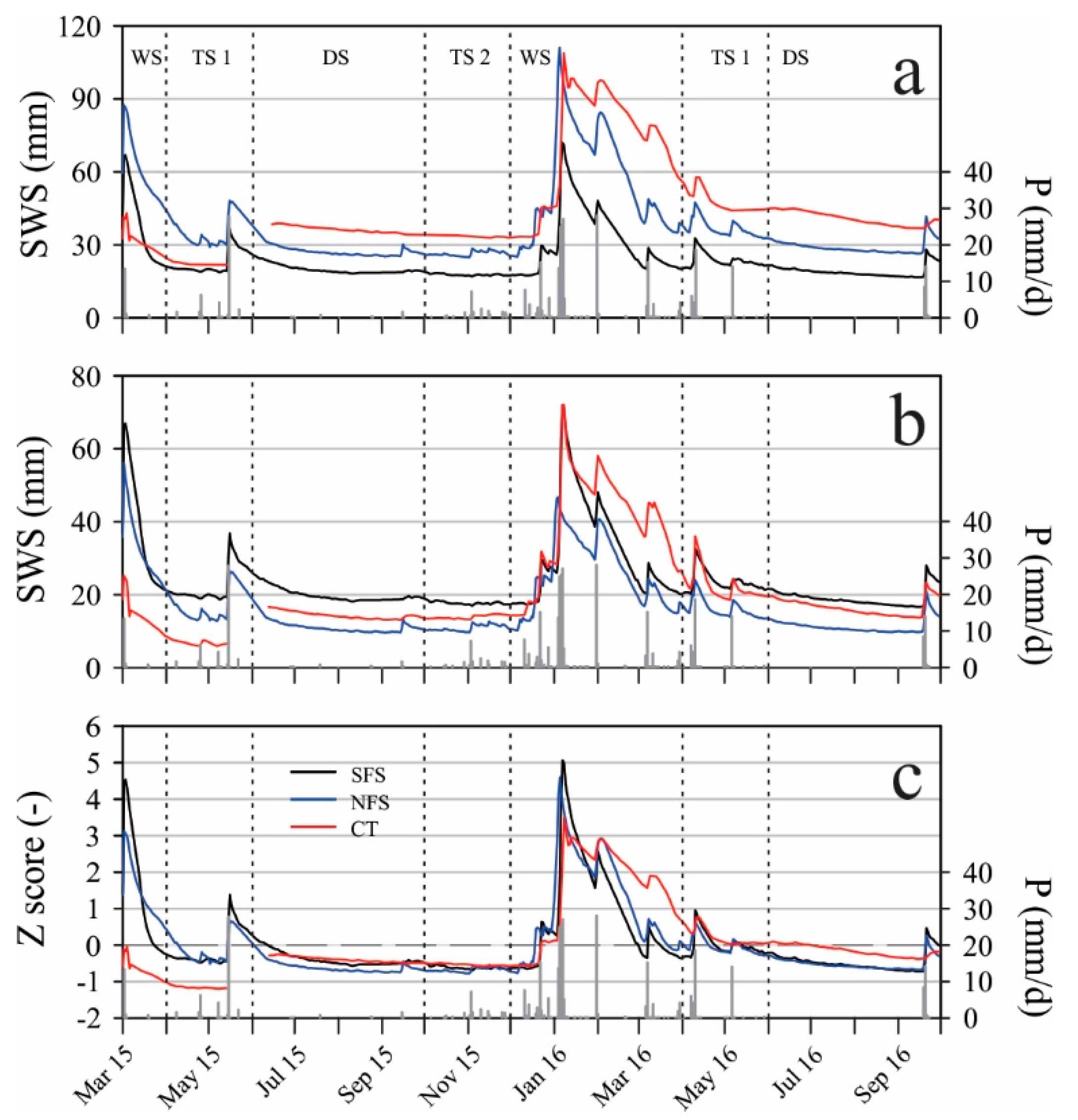
3.4. Comparison of Soil Water Storage Profiles Across Sites

Statistical descriptions of soil water storage (SWS) (up to 1 m at NFS and CT sites, and up to 0.4 m at SFS site) in each profile during the hydrological seasons are presented in

Table 2. Comparison of statistical values of SWS (mm) of each site and hydrological season up to 1 m depth at NFS and CT and 0.4 m at SFS: Min (minimum), Max (maximum), Avg (average), and Avg total (total average).

Stats	Site	WS-15	TS1-15	DS-15	TS2-15	WS-16	TS1-16	DS-16	Avg Total
Min	SFS	21	19	18	17	17	20	17	18
	NFS	45	29	25	25	25	33	26	30
	CT	25	21	32	33	33	44	36	32
Max	SFS	67	37	26	19	72	33	28	40
	NFS	87	48	38	29	111	47	41	57
	CT	43	32	39	34	109	59	45	51
Avg	SFS	37	23	20	18	32	24	19	25
	NFS	61	36	28	26	56	37	29	39
	CT	31	23	36	34	70	48	41	40

. Comparisons across sites are possible for the overlapping periods from WS-15 to DS-16 in terms of average profile water stored conditions. The highest values of SWS occurred during the winter months (rainy season). The NFS and CT sites showed the highest values (39 and 40 mm) over the entire period, and about 37% more SWS than the SFS site (25 mm). This indicates the NFS and CT sites exhibited higher soil water storage capacity over the entire profile. The highest average values of profile water stored during the WS-15 occurred at the hillslope sites (NFS, 61 mm; SFS, 37 mm), while the flat area (CT, 31 mm) exhibited lower values during this hydrological season. As an opposite case, it was observed during the following rainy season (WS-16) that the flat site (CT, 70 mm) had an accumulation of water stored higher than the hillslopes sites (NFS, 56 mm; SFS, 32 mm) (Table 2). Relating the SWS in the three soil profiles, we found that south-facing slope has persistently lower amounts of SWS than north-facing slope and CT site (Figure 7a; Table 2). This suggests that the aspect and slope effects on soil moisture are consistent with expectations in semiarid Mediterranean regions. Some studies have reported that south-facing slopes tend to be drier with lower infiltration rates [30,61,62,63].

Subsequently, temporal SWS patterns were compared under the same soil profile depth at the three sites (up to 0.4 m) (

Table 3. Comparison of statistical values of SWS (in mm) of each site and hydrological season up to 0.4 m depth: Min (minimum), Max (maximum), Avg (average), and Avg total (total average).

Stats	Site	WS-15	TS1-15	DS-15	TS2-15	WS-16	TS1-16	DS-16	Avg Total
Min	SFS	21	19	18	17	17	20	17	18
	NFS	22	13	10	10	10	13	10	13
	CT	9	6	13	13	14	18	14	12
Max	SFS	67	37	26	19	72	33	28	40
	NFS	56	26	18	13	47	24	21	29
	CT	25	13	17	15	72	36	23	29
Avg	SFS	37	23	20	18	32	24	19	25
	NFS	33	17	11	11	26	16	11	18
	CT	14	8	14	14	39	22	16	18

). The average totals of SWS up to 0.4 m, in this case, reveals that south-facing slope allowed more SWS than north-facing slope and CT in the entire period excepting in WS-16 in which CT was more representative. We attribute SWS amount at SFS site due to the lack of vegetation cover, which permits additional water to reach the soil surface and possible lateral subsurface water transport from uphill locations along the soil–bedrock interface.

To further investigate the SWS at hillslope and flat sites, Figure 7 presents the daily variation of SWS profile (Figure 7a), daily variation of SWS up to 0.4 m profile (Figure 7b) and the corresponding standardized values to detect trends equivalent to relatively wetter and drier soil profile regimes (Figure 7c). Dry periods are those whose SWS is lower than the standardized value of Z = 0 (Figure 7c). In general, the soil moisture that accumulates during the winter season dominates the overall wetter conditions of the hydrological seasons in all three sites (Figure 7a,b). An analysis of Pearson’s correlation coefficient indicates that there was a positive linear relation between SWS at the sites due to the probable common presence of precipitation pulses, similar soil textural characteristics, topographical features (SFS and NFS) and common presence of plant cover (at NFS and CT sites): SFS-NFS (R² = 0.92), SFS-CT (R² = 0.61) and NFS-CT (R² = 0.67).

The SWS up to 0.4 m was superior at SFS site than NFS for the entire period and greater than CT excluding WS-16 (Figure 7b). At SFS site, soil water content was highly enriched in the deepest layer (0.4 m), potentially due to rapid flow into the layer from local changes in the soil–bedrock configuration. As a result, increased SWS at SFS persisted along the hydrologic seasons.

A comparison across stations indicated wetter standardized conditions at SFS during rainfall peaks in winter (WS) and wet–dry transition (TS1) seasons in nearly all occurrences as compared to NFS, but soil water depletion occurs more quickly. Likewise, during a prolonged period in WS-16, CT exhibited higher standardized values than the other sites, suggesting water inputs from local precipitation or precipitation excess from surrounding areas. Soil water depletion occurred more rapidly at SFS and NFS during this period with durations of approximately 1 month (Figure 7c), due to steeper slopes and predominance of sandy fractions.

Overall, the soil moisture dynamics in each profile were consistent with prior Mediterranean climate studies showing that soils are generally saturated in the winter and exhibit recessions during the intervening dry periods (e.g., [4,64]). At our sites, dry soil conditions were persistent and lasted for nearly 70% of the time. Furthermore, if precipitation pulses were smaller than 7 mm during the transition seasons, dry conditions extended through those periods. Interestingly, the dry periods did not seem to reset the soil moisture differences across sites that were established during the wet winter seasons. As a result, the north and south-facing slopes had a wetter standardized conditions during P events followed by a faster depletion and the flat area permitted progressive accumulation of SWS after P events which depleted at a slower rate. Above average wet periods could also lead to much higher wetness at the flat CT site as compared to the hillslope locations.

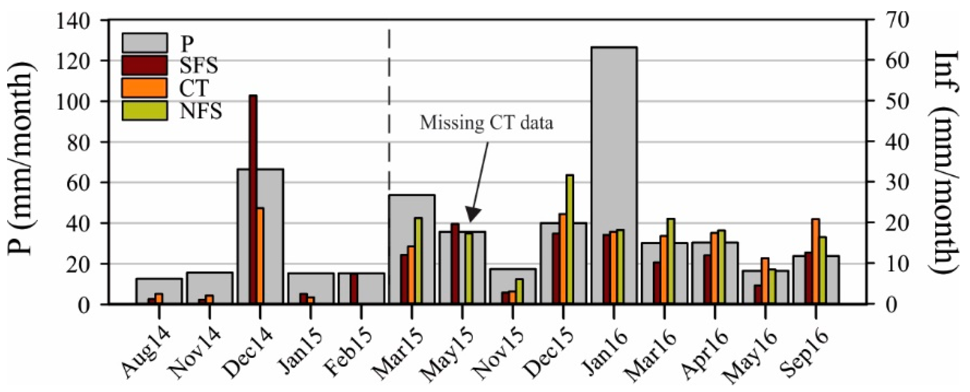
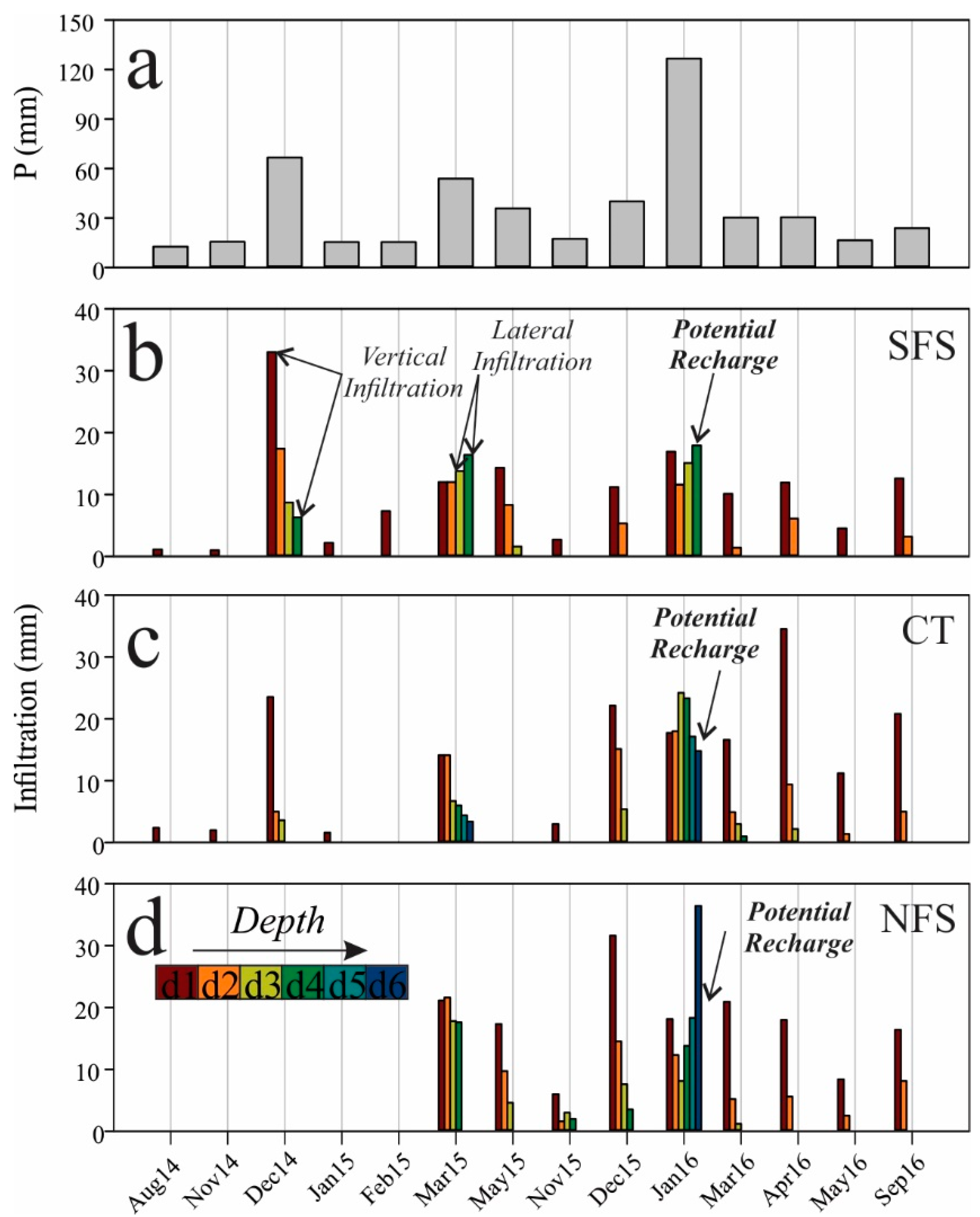
3.5. Infiltration and Potential Recharge During Precipitation Events

Vertical infiltration that reached 0.1 m depth, was estimated at each station for precipitation events larger than 7 mm during the study period. We estimate vertical infiltration in only 14 months, however, the comparison between the totals of the three stations was made since March 2015 to September 2016 (total P = 374 mm) (Figure 8). Figure 8 shown monthly precipitation and monthly infiltration at each site. As a result, at the three sites, monthly totals shown that between 28 and 42% of monthly P was vertically infiltrated into the top soil layer profiles (SFS < CT < NFS) and between 72 (SFS) and 58% (NFS) of the precipitation was lost to other superficial processes such as rainfall interception (not at SFS), evaporation and runoff (SFS > CT > NFS).

In Figure 9a,b, we show the nineteen precipitation events that occurred in the fourteen months under analysis. The cumulative precipitation, precipitation intensities, duration and vertical infiltration for each precipitation event was estimated since March 2015. It is interesting to note the totals of the precipitation-infiltration analysis revealed that water loss at ~0.1 m depth was lower at SFS than NFS and CT (between 15 and 20%,) this mechanism could be driven by a transpiration process at NFS and CT.

Furthermore, we found the fraction of infiltration that passed to underlying soil layers required precipitation events greater than ~10.5 mm for infiltration fronts to pass below the shallow soil layer (underneath 0.1 m; about ~10% of annual P events). Successive events with accumulations between 48 mm (December 2014) and 104 mm (January 2016) (Figure 9a) were needed for θ to increase in deeper layers (Figure 10). When precipitation events were intense (e.g., March 2015, 12 mm/h; 6 January 2016, 15.2 mm/h; 31 January 2016, 12.6 mm/h; Figure 9b; white circles), infiltration was limited substantially because the precipitation rate was greater than the capacity of the soil to transport vertical flow (Figure 10). On the other hand, during a sequence of low-intensity pulses (e.g., December 2014; Figure 9b), infiltration occurred progressively and the wetting front passed gradually to lower layers [60,65]. This mechanism was appreciated mainly during DS and the intermediate seasons TS1 and TS2 without the soil water content reaching the deepest soil layer (Figure 10).

Figure 10 presents infiltration estimates for each soil layer across all selected precipitation events, infiltration patterns (vertical and lateral) and potential recharge. In general, the infiltration decreased with soil depth with most events only having the wetting front reach within the top 0.2 m (d1 and d2). From March 2015, the largest events of P (March 2015, 53.8 and January 2016, 126.6 mm) (Figure 8) led to infiltration reaching the deepest soil layer at hillslope sites and were considered as potentially leading to recharge (Figure 10b, green bar; Figure 10d, dark blue bar). We calculated that these two precipitation events in total generated 34.4 mm considered as potential recharge at SFS site (March 2015, 16.4 mm; January 2016, 18 mm) (Figure 10b; green bars “d4”), 18.3 mm at CT site (March 2015, 3.4 mm; January 2016, 14.9 mm) and 36.5 mm at NFS site (January 2016) (Figure 10c,d; dark blue bars “d6” for CT and NFS). Overall, we estimated that on average about 9.5% of the accumulated precipitation (~374 mm; from March 2015 to September 2016) could contribute to the recharge of the mountain block aquifer at the two sites with opposing aspects (SFS and NFS; 34.5 mm average potential recharge). It is worth mentioning that SFS with less precipitation amounts allows infiltration water to reach the deepest layer of the soil profile, leading to greater probability of potential recharge in that site (e.g., March 2015 = 53.8 mm; Figure 10b) than the opposite NFS (with this amount of P, wetting front could not reach to the last layer “d6”).

4. Conclusions

This study presents a comparison of soil water content measurements, soil water storage, infiltration and potential recharge at three sites representing different topographic positions in a mountain block within a semiarid Mediterranean climate ecosystem. Results of the study reveal:

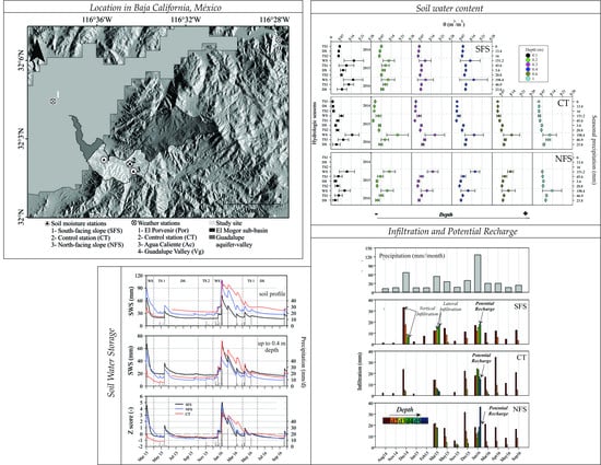
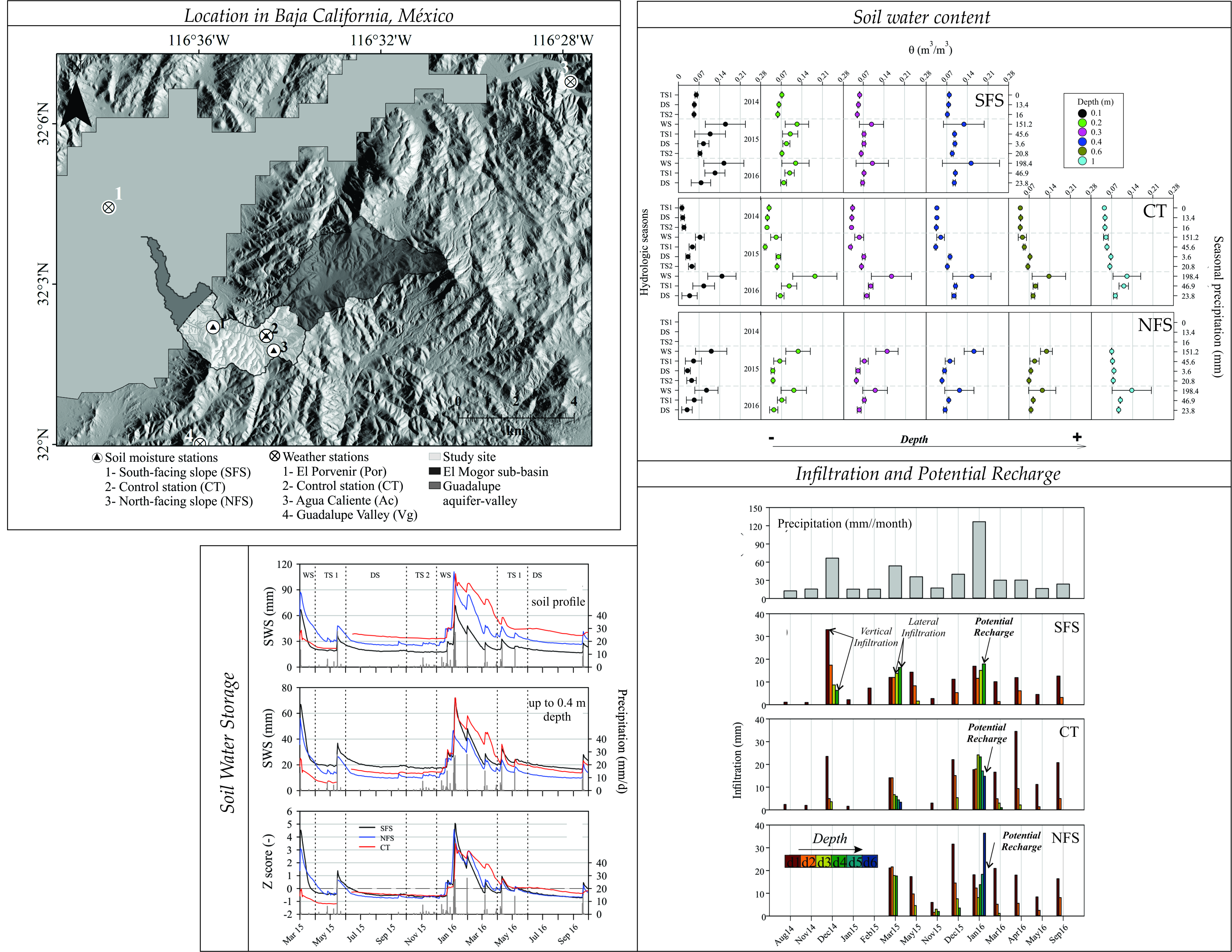
• The evolution of soil water content showed a strong variability on the opposing hillslopes (SFS and NFS) principally in the winter and wet–dry transition seasons in the shallowest depths. Likewise, the hillslope sites exhibit a sudden increase in soil water content during P peaks followed by rapid depletion. In contrast, the flatter site (CT) showed slower soil water content decreases and the accumulation of water from upland areas during significant events. During high-intensity P events, sites with opposing aspects reveal an increase of soil water content at the soil–bedrock interface (~0.4 m in SFS; ~1 m in NFS) suggesting lateral subsurface fluxes, while vertical soil infiltration decreases noticeably, signifying the production of surface runoff.
• The seasonal patterns of SWS were similar at the three sites. Precipitation in winter (WS) and wet–dry transition months (TS1) replenish SWS at each location, which is depleted in the summer–fall months most notably at the hillslope sites. NFS and CT sites exhibit relatively high SWS due to their larger soil profile thickness, but SWS comparison until 0.4 m revealed higher values at SFS sites. This is attributed to the lack of vegetation cover, which permits additional water to reach the soil surface and infiltrate in vertical and horizontal directions, and the possible effect of lateral subsurface water transport from uphill locations at the soil–bedrock interface.
• The relation of SWS at hillslope sites showed strong positive correlation. Soil water storage was completely depleted in the soil profiles at hillslope sites after WS, meaning that there is no water available in the soil until the next WS. Water deficit occurred in summer months (DS) and dry–wet transition months (TS2) and lasted for nearly 70% of the study period at the three sites.
• Potential recharge occurred only in WS with P events greater than 50 mm/month at SFS site and greater than 120 mm/month at NFS site, indicating that soil depth and lack of vegetation cover play a critical role in the transport of water towards the soil–bedrock interface. We calculate that on average, around 9.5% of accumulated precipitation (~374 mm; from March 2015 to September 2016) could contribute to the recharge of the aquifer by the two sites with opposing aspects (~34.5 mm).

The results presented here provide insights into the dynamics, storage and transport of soil water content at different temporal scales. This is the first research work carried out with these objectives in the region, and although results are spatially limited, they allow inferences to be made about the potential contribution of the hillslopes sites towards aquifer recharge in the mountain block.

References

1. Ines, A.V.M.; Mohanty, B.P. Near-surface soil moisture assimilation for quantifying effective soil hydraulic propertis using generic algorithm: 1. Conceptual modeling. Water Resour. Res. 2008, 44, W06422. [Google Scholar] [CrossRef]
2. Phuong Tran, A.; Bogaert, P.; Wiaux, F.; Vanclooster, M.; Lambot, S. High-resolution space-time quantification of soil moisture along a hillslope using joint analysis of ground penetrating radar and frequency domain reflectometry data. J. Hydrol. 2015, 523, 252–261. [Google Scholar] [CrossRef]
3. Gomez-Plaza, A.; Alvarez-Rogel, J.; Albaladejo, J.; Castillo, V.M. Spatial patterns and temporal stability of soil moisture across a range of scales in a semi-arid environment. Hydrol. Process. 2000, 14, 1261–1277. [Google Scholar] [CrossRef]
4. Martínez-Fernández, J.; Ceballos, A. Temporal stability of soil moisture in a large-field experiment in Spain. Soil Sci. Soc. Am. J. 2003, 67, 1647–1656. [Google Scholar] [CrossRef]
5. Vivoni, E.R.; Rinehart, A.J.; Mendez-Barroso, L.A.; Aragon, C.A.; Bisht, G.; Cardenas, M.B.; Engle, E.; Forman, B.A.; Frisbee, M.D.; Gutierrez-Jurado, H.A.; et al. Vegetation controls on soil moisture distribution in the Valles Caldera, New Mexico, during the North American monsoon. Ecohydrology 2008, 1, 225–238. [Google Scholar] [CrossRef]
6. Anenkhonov, O.A.; Korolyuk, A.Y.; Sandanov, D.V.; Liu, H.; Zverev, A.A.; Guo, D. Soil-moisture conditions indicated by field-layer plants help identify vulnerable forests in the forest-steppe of semi-arid Southern Siberia. Ecol. Indic. 2015, 57, 196–207. [Google Scholar] [CrossRef] [Green Version]
7. Zhang, T.; Berndtsson, R. Temporal patterns and spatial scale of soil water variability in a small humid catchment. J. Hydrol. 1988, 104, 111–128. [Google Scholar] [CrossRef]
8. Cantón, Y.; Solé-Benet, A.; Domingo, F. Temporal and spatial patterns of soil moisture in semiarid badlands of SE Spain. J. Hydrol. 2004, 285, 199–214. [Google Scholar] [CrossRef]
9. Cleverly, J.; Eamus, D.; Restrepo Coupe, N.; Chen, C.; Maes, W.; Li, L.; Faux, R.; Santini, S.N.; Rumman, R.; Yu, Q.; et al. Soil moisture controls on phenology and productivity in semi-arid critical zone. Sci. Total Environ. 2016, 568, 1227–1237. [Google Scholar] [CrossRef]
10. Zhao, Y.; Peth, S.; Wang, X.Y.; Lin, H.; Horn, R. Controls of surface soil moisture spatial patterns and their temporal stability in a semi-arid steppe. Hydrol. Process. 2010, 24, 2507–2519. [Google Scholar] [CrossRef]
11. Choi, M.; Jacobs, J.M. Soil moisture variability of root zone profiles within SMEX02 remote sensing footprints. Adv. Water Resour. 2007, 30, 883–896. [Google Scholar] [CrossRef]
12. Gao, L.; Shao, M.; Peng, X.; She, D. Spatio-temporal variability and temporal stability of water contents distributed within soil profiles at a hillslope scale. Catena 2015, 132, 29–36. [Google Scholar] [CrossRef] [Green Version]
13. Zhou, J.; Fu, B.; Gao, G.; Lü, N.; Lü, Y.; Wang, S. Temporal stability of surface soil moisture of different vegetation types in the Loess Plateau of China. Catena 2015, 128, 1–15. [Google Scholar] [CrossRef] [Green Version]
14. Porporato, A.; Laio, F.; Ridolfi, L.; Rodriguez-Iturbe, I. Plants in water-controlled ecosystems: Active role in hydrologic processes and response to water stress: III. Vegetation water stress. Adv. Water Resour. 2001, 24, 725–744. [Google Scholar] [CrossRef]
15. Legates, D.R.; Mahmood, R.; Levia, D.F.; DeLiberty, T.L.; Quiring, S.M.; Houser, C.; Nelson, F.E. Soil moisture: A central and unifying theme in physical geography. Prog. Phys. Geogr. 2011, 35, 65–86. [Google Scholar] [CrossRef]
16. Yang, L.; Wei, W.; Chen, L.; Chen, W.; Wang, J. Response of temporal variation of soil moisture to vegetation restoration in semi-arid Loess Plateau, China. Catena 2014, 115, 123–133. [Google Scholar] [CrossRef] [Green Version]
17. Reynolds, J.F.; Kemp, P.R.; Ogle, K.; Fernández, R.J. Modifying the pulse-reserve paradigm for deserts of North America: Precipitation pulses, soil water and plant responses. Oecología 2004, 141, 194–210. [Google Scholar] [CrossRef]
18. Vivoni, E.R.; Gutiérrez-Jurado, H.A.; Aragón, C.A.; Méndez-Barroso, L.A.; Rinehart, A.J.; Wyckoff, R.L.; Rodríguez, J.C.; Watts, C.J.; Bolten, J.D.; Lakshmi, V.; et al. Variation of hydrometeorological conditions along a topographic transect in northwestern Mexico during the North American monsoon. J. Clim. 2007, 20, 1792–1809. [Google Scholar] [CrossRef]
19. Del Toro-Guerrero, F.J.; Kretzschmar, T.; Hinojosa-Corona, A. Hydric balance in a semi-arid basin, El Mogor, Baja California, Mexico. Technol. Water Sci. 2014, 5, 69–81. (In Spanish) [Google Scholar]
20. Foster, S.S.D.; Smith-Carington, A. The interpretation of tritium in the chalk unsaturated zone. J. Hydrol. 1980, 46, 343–364. [Google Scholar] [CrossRef]
21. Phillips, F.M. Environmental tracers for water movement in desert soils of the American Southwest. Soil Sci. Soc. Am. J. 1994, 58, 15–24. [Google Scholar] [CrossRef]
22. Izbicki, J.A.; Radyk, J.; Michel, R.L. Water movement through a thick unsaturated zone underlying an intermittent stream in the western Mojave Desert, Southern California, USA. J. Hydrol. 2000, 238, 194–217. [Google Scholar] [CrossRef]
23. Walvoord, M.A.; Plummer, M.A.; Phillips, F.M. Deep arid system hydrodynamics 1. Equilibrium states and response times in thick desert vadose zones. Water Resour. Res. 2002, 38, 1–15. [Google Scholar] [CrossRef]
24. Wilson, J.L.; Guan, H. Mountain-Block hydrology and Mountain-Front recharge. In Groundwater Recharge in a Desert Environment: The Southwestern United States; Phillips, F.M., Hogan, J., Scanlon, B., Eds.; AGU: Washington, DC, USA, 2004; pp. 113–138. [Google Scholar]
25. Gutiérrez-Jurado, H.A.; Vivoni, E.R.; Harrison, J.B.J.; Guan, H. Ecohydrology of root zone water fluxes and soil development in complex semiarid rangelands. Hydrol. Processes 2006, 20, 3289–3316. [Google Scholar] [CrossRef]
26. Gutiérrez-Jurado, H.A.; Vivoni, E.R.; Cikoski, C.; Harrison, J.B.J.; Bras, R.L.; Istanbulluoglu, E. On the observed ecohydrologic dynamics of a semiarid basin with aspect-delimited ecosystems. Water Resour. Res. 2013, 49, 8263–8284. [Google Scholar] [CrossRef] [Green Version]
27. Bennie, J.; Hill, M.O.; Baxter, R.; Huntley, B. Influence of slope aspect on long-term vegetation change in British chalk grasslands. J. Ecol. 2006, 94, 355–368. [Google Scholar] [CrossRef]
28. Warren, R.J. An experimental test of well-described vegetation patterns across slope aspects using woodland herb transplants and manipulated abiotic drivers. New Phytol. 2010, 185, 1038–1049. [Google Scholar] [CrossRef] [Green Version]
29. Dubayah, R.; Rich, P.M. GIS-based solar radiation modeling. In GIS and Environmental Modeling: Progress and Research Issues; Goodchild, M.F., Steyaert, L.T., Parks, B.O., Johnston, C., Maidment, D., Crane, M., Glendinning, S., Eds.; GIS World Books: Fort Collins, CO, USA, 1996; pp. 129–137. [Google Scholar]
30. Bennie, J.; Huntley, B.; Wiltshire, A.O.; Hill, M.; Baxter, R. Slope, aspect and climate: Spatially explicit and implicit models of topographic microclimate in chalk grassland. Ecol. Model. 2008, 216, 47–59. [Google Scholar] [CrossRef]
31. Albaba, I. The effects of slope orientations on vegetation characteristics of Wadi Alquf forest reserve (WAFR) West Bank-Palestine. Int. J. Agric. Soil Sci. 2014, 2, 118–125. [Google Scholar]
32. Del Toro-Guerrero, F.J.; Hinojosa-Corona, A.; Kretzschmar, T. A comparative study of NDVI values between North-and South-Facing slopes in a semiarid mountainous region. IEEE J. Sel. Top. Appl. Earth Obs. Remote Sens. 2016, 9, 5350–5356. [Google Scholar] [CrossRef]
33. Kurczyn-Robledo, A.; Kretzschmar, T.; Hinojosa-Corona, A. Surface runoff evaluation in the northwest of Guadalupe Valley, B.C., México, using the numbered curves method and satellite data. Rev. Mex. Cienc. Geol. 2007, 24, 1–14. (In Spanish) [Google Scholar]
34. Del Toro-Guerrero, F.J.; Kretzschmar, T. Identifying periods of historical drought in a region of semiarid mediterranean climate type. Rev. Mex. Cienc. Agríc. 2016, 7, 1311–1320. [Google Scholar] [CrossRef]
35. Flores-Zavala, R. Evaporación y Transpiración Según tres Patrones Espaciales y Estacionales en un Ecosistema Mediterráneo en la Subcuenca de El Mogor, Ensenada, Baja California. Tesis de Maestría, Centro de Investigación Científica y de Educación Superior de Ensenada, Baja California (CICESE), Ensenada, Mexico, 2016; p. 36. [Google Scholar]
36. Villarreal, S.; Vargas, R.; Yepez, E.A.; Acosta, J.S.; Castro, A.; Escoto-Rodriguez, M.; Lopez, E.; Martínez-Osuna, J.; Rodriguez, J.C.; Smith, S.V.; et al. Contrasting precipitation seasonality influences evapotranspiration dynamics in water-limited shrublands. J. Geophys. Res. Biogeosci. 2016, 121, 494–508. [Google Scholar] [CrossRef]
37. Pražnikar, J. Particulate matter time-series and Köppen-Geiger climate classes in North America and Europe. Atmos. Environ. 2017, 150, 136–145. [Google Scholar] [CrossRef]
38. Castro-Escárrega, J.J.; Terán-Martínez, G.E.; Siqueiros-López, C. Geological-Mining Chart Tijuana I11-11 Baja California. Mexican Geological Service. 2003. Available online: http://www.sgm.gob.mx (accessed on 12 June 2018).
39. Mexican National Institute of Statistics and Geography (INEGI). High Resolution Digital Elevation Model LiDAR, Terrain Type; I11D82XX (Data and Metadata); INEGI: Baja California, Mexico, 2008. [Google Scholar]
40. Beven, K.J.; Kirkby, M. A physical based variable contributing area model of basin hydrology. Hydrol. Sci. Bull. 1979, 24, 43–79. [Google Scholar] [CrossRef]
41. International Atomic Energy Agency (IAEA). Field Estimation of Soil Water Content; IAEA: Vienna, Austria, 2008; p. 131. [Google Scholar]
42. Qi, Z.; Helmers, M.J. The conversion of permittivity as measured by a PR2 capacitance probe into soil moisture values for Des Moines lobe soils in Iowa. Soil Use Manag. 2010, 26, 82–92. [Google Scholar] [CrossRef]
43. Kargas, G.; Kerkides, P.; Pouovassilis, A. Infiltration of rain water in semi-arid areas under three land surface treatments. Soil Tillage Res. 2012, 120, 15–24. [Google Scholar] [CrossRef]
44. Delta T-Devices, Ltd. User Manual for the Profile Probe Type PR2; Delta T-Devices, Ltd.: Cambridge, UK, 2016. [Google Scholar]
45. Green, W.H.; Ampt, G.A. Studies in soil physics. I. The flow of air and water through soils. J. Agric. Sci. 1911, 4, 1–24. [Google Scholar] [CrossRef]
46. Bhark, E.W.; Small, E.E. Association between plant canopies and the spatial patterns of infiltration in shrubland and grassland of the Chihuahuan Desert, New Mexico. Ecosystems 2003, 6, 185–196. [Google Scholar] [CrossRef]
47. Moran, M.S.; Hamerlynck, E.P.; Scott, R.L.; Stone, J.J.; Holifield Collins, C.D.; Keefer, T.O.; Bryant, R.; DeYoung, L.; Nearing, G.S.; Sugg, Z.; et al. Hydrologic response to precipitation pulses under and between shrubs in the Chihuahuan Desert, Arizona. Water Resour. Res. 2010, 46, 1–12. [Google Scholar] [CrossRef]
48. Zakharov, S.A. Importance of slope aspect and gradient for soil and vegetation distribution in the Great Caucasus. Bot. J. Acad. Sci. USSR 1940, 25, 378–405. [Google Scholar]
49. Florinsky, I.V. Digital Terrain Analysis in Soil Science and Geology, 2nd ed.; Academic Press-Elsevier: London, UK, 2016; p. 486. [Google Scholar]
50. Willgoose, G.; Hancock, G. Revisiting the hypsometric curve as an indicator of form and process in transport-limited catchment. Earth Surf. Process. Landf. 1998, 23, 611–623. [Google Scholar] [CrossRef]
51. Kirkby, M.J.; Chorley, R.J. Throughflow, overland flow and erosion. Bull. Int. Assoc. Sci. Hydrol. 1967, 12, 5–21. [Google Scholar] [CrossRef]
52. Hu, W.; Shao, M.A.; Reichardt, K. Using a new criterion to identify sites for mean soil water storage evaluation. Soil Sci. Soc. Am. J. 2010, 74, 762–773. [Google Scholar] [CrossRef]
53. Gao, L.; Shao, M. Temporal stability of soil water storage in diverse soil layers. Catena 2012, 95, 24–32. [Google Scholar] [CrossRef]
54. Penna, D.; Brocca, L.; Borga, M.; Dalla Fontana, G. Soil moisture temporal stability at different depths on two alpine hillslopes during wet and dry periods. J. Hydrol. 2013, 477, 55–71. [Google Scholar] [CrossRef]
55. Gutiérrez-Jurado, H.A.; Vivoni, E.R.; Istanbulluoglu, E.; Bras, R.L. Ecohydrological response to a geomorphically significant flood event in a semiarid catchment with contrasting ecosystems. Geophys. Res. Lett. 2007, 34, L24S25. [Google Scholar] [CrossRef]
56. Rosenbaum, U.; Bogena, H.R.; Herbst, M.; Huisman, J.A.; Peterson, T.J.; Weuthen, A.; Western, A.W.; Vereecken, H. Seasonal and event dynamics of spatial soil moisture patterns at the small catchment scale. Water Resour. Res. 2012, 48, 1–22. [Google Scholar] [CrossRef]
57. Jia, X.; Shao, M.; Wei, X.; Wang, Y. Hillslope scale temporal stability of soil water storage in diverse soil layers. J. Hydrol. 2013, 498, 254–264. [Google Scholar] [CrossRef]
58. McIntosh, J.; McDonnell, J.J.; Peters, N.E. Tracer and hydrometric study of preferential flow in large undisturbed soil cores from the Georgia Piedmont, USA. Hydrol. Process. 1999, 13, 139–155. [Google Scholar] [CrossRef]
59. Lin, H.; Zhou, X. Evidence of subsurface preferential flow using soil hydrologic monitoring in the Shale Hills catchment. Eur. J. Soil Sci. 2008, 59, 34–49. [Google Scholar] [CrossRef]
60. Takagi, K.; Lin, H.S. Changing controls of soil moisture spatial organization in the Shale Hills Catchment. Geoderma 2012, 173–174, 289–302. [Google Scholar] [CrossRef]
61. Famiglietti, J.S.; Rudnicki, J.W.; Rodell, M. Variability in surface moisture content along a hillslope transect: Rattlesnake Hill, Texas. J. Hydrol. 1998, 210, 259–281. [Google Scholar] [CrossRef] [Green Version]
62. Brocca, L.; Morbidelli, R.; Melone, F.; Moramarco, T. Soil moisture spatial variability in experimental areas of central Italy. J. Hydrol. 2007, 333, 356–373. [Google Scholar] [CrossRef]
63. Moeslund, J.E.; Arge, L.; Bocher, P.K.; Dalgaard, T.; Odgaard, M.V.; Nygaard, B.; Svenning, J. Topographically controlled soil moisture is the primary driver of local vegetation patterns across a lowland region. Ecosphere 2013, 4, 91. [Google Scholar] [CrossRef]
64. Ceballos, A.; Martínez-Fernández, J.; Santos, F.; Alonso, P. Soil-water behavior of sandy soils under semi-arid conditions in the Duero Basin (Spain). J. Arid Environ. 2002, 51, 501–519. [Google Scholar] [CrossRef]
65. Grayson, R.B.; Western, A.W.; Chiew, H.S.; Blöschl, G. Preferred states in spatial soil moisture patterns: Local and nonlocal controls. Water Resour. Res. 1997, 33, 2808–2897. [Google Scholar] [CrossRef]
Figure 1. (a) Location of the study site in Baja California, Mexico. (b) Shaded relief map, with monitoring sites and surrounding weather stations shown. (c) South-facing slope (SFS), control (CT) and north-facing slope (NFS) micro-basins are presented.
Water 10 01844 g001
Figure 2. Contrasts between vegetation on north-facing slopes (NFS), south-facing slopes (SFS) and control (CT) sites during the wet season.
Water 10 01844 g002
Figure 3. (a) Comparative analysis of monthly and annual precipitation patterns between CT (black bars), Guadalupe Valley (Vg; gray bars), (b) El Porvenir (Por; black bars) and Agua Caliente (Ac; gray bars) weather stations with information from 2012–2016.
Water 10 01844 g003
Figure 4. Topographic indices and morphometric analysis derived from a 5 m digital terrain model for the SFS, CT and NFS micro-basins and its relation with respective area: (a) hypsometry, (b) slope, (c) aspect, (d) topographic wetness index (TWI) and (e) curvature. Vertical solid lines represent morphometric values at soil moisture stations and circles represents mean morphometric values of each micro-basin.
Water 10 01844 g004
Figure 5. (a) Daily precipitation. (bg) Daily-averaged soil water content at depths of 0.1 m, 0.2 m, 0.3 m, 0.4 m, 0.6 m and 1 m for each site. Dashed vertical lines indicate the hydrological seasons.
Water 10 01844 g005
Figure 6. Relation of seasonal evolution of average θ in the hydrological seasons at different depths and the seasonal precipitation at sites: (a) SFS, (b) CT and (c) NFS. The horizontal dashed lines represent the boundary between the hydrological years and the lines in the circles represent the seasonal standard deviation.
Water 10 01844 g006
Figure 7. (a) Daily soil water storage in each profile up to 1 m depth, (b) daily soil water storage in each profile up to 0.4 m depth and (c) standardized daily SWS (Z) value for each profile-site, along with daily precipitation.
Water 10 01844 g007
Figure 8. Monthly precipitation at CT weather station and monthly infiltration at SFS, CT and NFS. The vertical discontinuous line represents the beginning of the comparative period of the three monitoring sites.
Water 10 01844 g008
Figure 9. (a) The measured precipitation (gray bars) and estimated vertical infiltration at 0.1 m depth (color bars) per event at the three monitoring sites. (b) The average and maximum precipitation intensity (black and white circles, respectively) and the time duration of the selected precipitation events (white bars). aP represents accumulated precipitation.
Water 10 01844 g009
Figure 10. (a) Accumulated monthly precipitation and (bd) total infiltration for each soil depth interval (d1 to d6) for events with P > 7 mm. Note that SFS is limited to 0.4 m (d4), while CT and NFS extend to 1 m (d6). SFS (b), CT (c) and NFS (d).
Water 10 01844 g010