Combining an R-Based Evolutionary Algorithm and Hydrological Model for Effective Parameter Calibration

Abstract

The hydrological model assessment and development (hydromad) modeling package is an R-based package that can be applied to simulate hydrological models and optimize parameters. As the hydromad package is incompatible with hydrological models outside the package, the parameters of such models cannot be directly optimized. Hence, we proposed a method of optimizing the hydrological-model parameters by combining the executable (EXE) file of the hydrological model with the shuffled complex evolution (SCE) algorithm provided by the hydromad package. A physically based, spatially distributed, grid-based rainfall–runoff model (GRM) was employed. By calibrating the parameters of the GRM, the performance of the model was found to be reasonable. Thus, the hydromad can be used to optimize the hydrological-model parameters outside the package if the EXE file of the hydrological model is available. The time required to optimize the parameters depends on the type of event, even for the same catchment area.

1. Introduction

Theoretically, a physically based, distributed hydrological model can be applied to simulate runoffs by extracting the required values of the parameters from the characteristics of a catchment, without requiring parameter calibration. However, the parameters are generally optimized using optimization algorithms because of factors such as spatial scale problems due to the difference between the scale of the measurement data and the model grid scale, error in the observed data, and lack of data for estimating parameters that are difficult to measure [1,2,3,4,5]. Moreover, it is difficult to incorporate various optimization algorithms into the modeling package when the number of parameters in the distributed hydrological model to be optimized is considerable. Therefore, previous studies have optimized the parameters of a distributed hydrological model using the trial-and-error method in cases where the required optimization algorithms were not included in the modeling package [6,7,8,9,10]. However, parameter calibration using the trial-and-error method can be time consuming; moreover, the reliability of the results is affected [3].

The hydrological model assessment and development (hydromad) [11] is a widely used R-based hydrological modeling package [12,13,14,15,16,17,18,19,20,21]. The hydromad package can be used to simulate conceptual hydrological models, optimize parameters, and analyze uncertainties. It provides various parameter optimization techniques. However, because the existing hydromad package is incompatible with hydrological models outside the package, the parameters of such models cannot be automatically optimized. To address this issue, several studies have optimized the parameters of the hydrological models using only the source code of the optimization algorithms provided in the hydromad package [22,23,24,25,26]. Hydromad is an open-source software package, which can be downloaded from http://hydromad.catchment.org.

The aim of this paper is to demonstrate that hydromad package can be used as a general auto calibration tool for hydrologic models. In this study, we used the R-based shuffled complex evolution (SCE) [27,28] algorithm code (SCEoptim) and a connection code (fitBySCE) included in the hydromad package. We demonstrated that the parameters of the distributed hydrological model could be estimated in a relatively easy manner by modifying the fitBySCE function and linking the executable (EXE) file of a distributed hydrological model outside the package with the SCEoptim. We employed the grid-based rainfall–runoff model (GRM) [29] for illustrative purposes. If a hydrological model other than the GRM has an EXE file (e.g., HEC-HMS, VIC, and HBV model) that can be executed in console window mode without graphical user interface (GUI), the parameters of the model can be calibrated using the R language-based SCE algorithm shown in this study. The GRM is available for free download at https://github.com/floodmodel/GRM.

The rest of this paper is organized as follows. Section 2 explains the SCE algorithm, the GRM used in this study, and the R-based interworking code. Section 3 introduces the catchments and the data inputted to the GRM. Section 4 presents the results and discussion. Finally, the conclusions of this study are given in Section 5.

2. Combining the R-Based SCE Algorithm and GRM

2.1. Shuffled Complex Evolution Algorithm

The SCE algorithm is one of the most widely used algorithms for parameter optimization [30] and has been used in various studies [31,32,33,34]. The SCE algorithm was developed using four different methods: Simplex procedure [35], controlled random search [36], competitive evolution [37], and complex shuffling [27]. The parameter optimization process of the algorithm is briefly described as follows. First, the initial population is randomly selected within a given parameter range. In the second step, the selected population is divided into complexes. Here, the complexes represent communities having parents who can reproduce an offspring. In the third step, each complex is independently evolved using a competitive complex evolution strategy. In the fourth step, all evolved complexes are mixed into a single population. This mixing process signifies the exchange of information. Finally, steps 2–4 are repeated until the pre-selected convergence condition is satisfied.

In this study, the convergence condition is met either if the difference between the objective functions of the previous and current iterations is lower than 0.00001 or if the pre-selected maximum number of iterations (herein five) is reached. The objective function used for the parameter optimization is the Nash–Sutcliffe efficiency (NSE) coefficient [38].

$$NSE=1-\frac{{\displaystyle {\sum }_{i=1}^n{\left(Q_{obs,i}-Q_{sim,i}\right)}^2}}{{\displaystyle {\sum }_{i=1}^n{\left(Q_{obs,i}-\overline{Q_{obs}}\right)}^2}}$$

(1)

where $Q_{obs,i}$ and $Q_{sim,i}$ are the observed and simulated runoffs at the ith time, respectively, and $\overline{Q_{obs}}$ denotes the mean value of the observed runoffs. The NSE values range from −∞ to 1, where 1 implies that the simulated and observed runoffs are equal. The objective function is obtained as the square of the difference between the observed and simulated values; therefore, it focuses on fitting larger flows in a hydrograph [39]. Thus, it is appropriate for simulating storm events, such as the ones presented in this study. Note that the SCE algorithm can automatically optimize the parameters of the hydrological model using various objective functions such as root mean squared error, relative bias, NSE using square-root transformed data, and NSE using log transformed data (see “Calculate objective function value” in Step 4 of Box A1 in Appendix A for usage of other objective functions). However, the purpose of this paper is to link the R-based SCE algorithm with the EXE file of the hydrological model. Thus, although additional objective functions can be used, this study is based on the use of one objective function for illustrative purposes. In addition, users can refer to the R code presented in this study and use additional objective functions for their research purposes.

In addition, we used correlation coefficient (CC) and normalized root mean square error (nRMSE) to investigate the fitness of simulated runoffs using the R-based SCE algorithm. Higher values of CC indicate more correlation between the observed and simulated runoffs, and lower values of nRMSE indicate less residual variance.

$$CC=\frac{Cov\left(Q_{obs},Q_{sim}\right)}{{\sigma }_{Q_{obs}}{\sigma }_{Q_{sim}}}$$

(2)

$$nRMSE=\frac{1}{Q_{obs,max}-Q_{obs,min}}\sqrt{\frac{{\displaystyle {\sum }_{i=1}^n{\left(Q_{obs,i}-Q_{sim,i}\right)}^2}}{n}}$$

(3)

where $Cov(Q_{obs},Q_{sim})$ is the covariance of the observed and simulated runoffs, ${\sigma }_{Q_{obs}}$ and ${\sigma }_{Q_{sim}}$ are the standard deviation of the observed and simulated runoff, respectively, and $Q_{obs,max}$ and $Q_{obs,min}$ are maximum and minimum value of the observed flow, respectively.

2.2. Grid-Based Rainfall–Runoff Model

The GRM is a grid-based, physically distributed, hydrological model used for simulating rainfall–runoff events. A kinematic wave model is used for the runoff analysis, and the Green–Ampt model [40] is used to simulate infiltration, sub-surface runoff, and baseflow. In addition, the effects of river-flow control facilities, such as dams and reservoirs, can be analyzed. The detailed theory and functions of the GRM are given in the manual provided by Choi and Kim [41].

The GRM is provided in the form of an EXE file, which runs in the console window mode. To run the model, the GRM project file (.gmp) is used as the switch argument. The GRM project file contains the path and the name of the input file used for the runoff simulation, modeling settings, and model parameters. Therefore, to execute the GRM using multiple parameter sets, it is necessary to either (1) prepare GRM project files corresponding to each parameter set in advance, or (2) perform the runoff analysis while dynamically modifying the parameters contained in a GRM project file. In this study, method (2) was applied.

Table 1. Parameters of the grid-based rainfall–runoff model (GRM) to be calibrated using the shuffled complex evolution (SCE) algorithm.

Parameter	Lower	Upper	Description
IniSaturation	0	1	Initial soil saturation ratio
MinSlopeOF	0.0001	0.01	Minimum slope of land surface
MinSlopeChBed	0.0001	0.01	Minimum slope of channel bed
ChRoughness	0.008	0.2	Channel roughness coefficient
CalCoefLCRoughness	0.6	1.3	Correction factor for land cover roughness coefficient
CalCoefPorosity	0.9	1.1	Correction factor for soil porosity
CalCoefWFSuctionHead	0.25	4	Correction factor for soil wetting front suction head
CalCoefHydraulicK	0.05	20	Correction factor for soil hydraulic conductivity
CalCoefSoilDepth	0.8	1.2	Correction factor for soil depth

lists the parameters to be calibrated and the physically applicable range of each parameter in this study.

2.3. Combination of the GRM and the SCE Algorithm

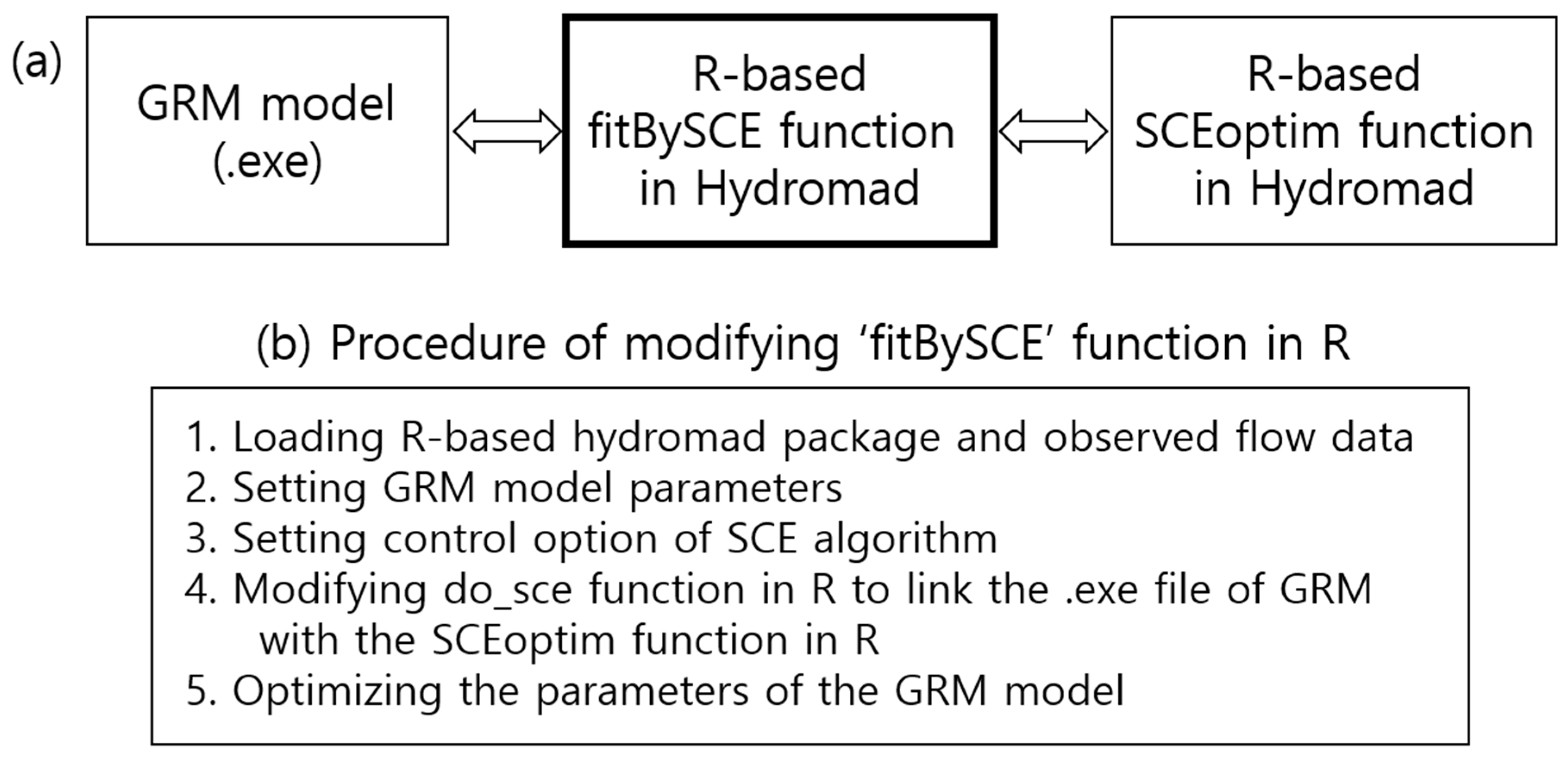
Figure 1 shows the schematic of the combination of the GRM and the SCE algorithm provided in the hydromad package and a brief description of the procedure for modifying the link code in R. The fitBySCE function in R in the hydromad package is used to link the SCEoptim function in R, i.e., the main code of the SCE algorithm, with the various hydrological models in the hydromad package. We modified the R code in the fitBySCE function to match the GRM with the SCEoptim function, as shown in Figure 1b and Box A1 in Appendix A. Steps 1–5 in Box A1 are identical to those shown in Figure 1b. The original codes for the fitBySCE and SCEoptim functions can be found on the hydromad website (http://hydromad.catchment.org).

The explanation of Box A1 in Appendix A, for the connection of GRM and SCEoptim function is as follows.

• First, users download the hydromad package from the website (http://hydromad.catchment.org) and install it. Users then use the “library” function to load the hydromad package. After that, users read the observed flow time series data for parameter calibration using R. The SCE algorithm adjusts the parameter values so that the simulated flow time series is as close as possible to this observed flow time series.
• Second, users set a range of parameters for the hydrological model using the R script in the second step. Since the SCE algorithm finds optimal parameter values within selected ranges of parameters, careful consideration should be given to whether the ranges of parameters are physically valid. Users can create a parameter list using the R script in the second step (see “parlist”) and set the upper, lower and initial values of the parameters for parameter calibration.
• Third, users can control the options of the SCE algorithm, such as the number of complexes and the maximum number of iterations. In this study, we used 20 number of complexes and 5 maximum number of iterations by considering the complexity of GRM. Users must select a function scale of −1 (see “control”) to ensure that the parameters have the optimal values when the value of the objective function is maximum. Users can also use the trace option to check the parameter tracking process in real time (see “control$trace”).
• The fourth step is the step of linking the EXE file of the GRM with the R-based SCE algorithm. Users can perform this process by modifying the source code of the R-based SCE algorithm in the hydromad package. For a detailed description of this step, first set the initial best model (“bestModel” that is a model simulation) and best objective function values (“bestFunVal”) using the R script (see “Set best model and best objective function values”). Then we modified the “do_sce” function in the hydromad package to update the GRM’s 9 initial parameter values to the GRM project file (.gmp) (see “Update GRM parameters” and “Read ‘.gmp’ file that contains information including parameter values and location of geophysical input data”). After that, we used the updated GRM parameters (ds500_E201107.gmp) and the EXE file of the GRM (GRM.exe) for GRM simulation by “system” function (see “Run GRM”). The result of GRM simulation is stored in “thisMod”. Then, the observed flow time series (Q) and simulated flow time series by GRM (X) are used to calculate the objective function value (“r.squared” that is the NSE of this study) by “hmadstat” function in the hydromad package. The calculated objective function value is stored in “thisVal”. If “thisMod” and “thisVal” are best values for each iteration, they are updated as “bestModel” and “bestFunVal”, respectively.
• Finally, the modified do_sce function, upper limit, lower limit, initial parameter values, and control option are put into the SCEoptim function and the optimal parameter values are estimated through the evolution process.

Note that the original function fitBySCE provided in the hydromad package is not used in this study, because we directly executed the script in terms of the modified fitBySCE function in R. The script in terms of the modified fitBySCE function (Box A1 in Appendix A) is represented as an example of an event.

3. Catchments and Input Data

3.1. Catchments

In this study, the Danseong and Seonsan catchments, which are major tributary catchments of the Nakdong River in South Korea, were selected for the calibration of the GRM, as shown in Figure 2. The area of the Danseong catchment is approximately 1710 km². Most regions in the Danseong catchment have steep mountains (approximately 73%), and agricultural land is distributed near the mountain stream (approximately 21%). The area of the Seonsan catchment is approximately 980 km², constituting approximately 65% of low mountainous area. Moreover, the farmland is relatively flat (approximately 28%) throughout the catchment, except in the mountainous regions. The Seonsan catchment is flatter than the Danseong catchment but is relatively closer to natural catchments and includes an urban area of approximately 4% of the catchment area.

3.2. Geographical and Hydrological Data

Table 2. Geographical and hydrological input data for the GRM.

Data (ASCII Raster)	Usage
DEM	Used in drainage analysis and to obtain the raster data (catchment, flow direction, flow accumulation, stream, and slope) for the GRM
Land cover map	Used to obtain the land cover data for the GRM
Detailed soil map	Used to obtain the soil texture and soil depth data for the GRM

lists the input data of the GRM used in this study. The GRM uses spatial information in raster format. The hydrological terrain factors, such as the catchment, flow direction, flow accumulation, stream, and slope layers were extracted from a digital elevation model (DEM), which is provided by the National Geographic Information Institute (http://www.ngii.go.kr). The land cover and soil information (soil texture and soil depth) were obtained with the help of the major land cover map (Ministry of Environment, http://www.me.go.kr) and a detailed soil map (National Academy of Agricultural Science, http://www.naas.go.kr) of South Korea, respectively. In this study, the spatial data were constructed in ASCII raster format with a resolution of 500 m × 500 m, for the two studied catchments.

Two storm events were selected for each study area (

Table 3. Storm events for each catchment.

Catchment	Event Number	Period	Rainfall (mm)	Peak Flow (m3/s)
Danseong	1	3 July 2011 20:00–5 July 2011 12:00	43	687
	2	14 July 2012 15:00–16 July 2012 15:00	63	1232
Seonsan	1	11 August 2010 00:00–12 August 2010 20:00	66	1361
	2	9 July 2011 11:00–12 July 2011 20:00	154	1814

). The average rainfall in each catchment was generated by the Thiessen Polygon method using the observed rainfall of the rainfall stations shown in Figure 2. These rainfall stations are operated by the Ministry of Land, Infrastructure and Transport (www.molit.go.kr). The time interval for the rainfall and flow data is 10 min.

4. Results and Discussion

Figure 3 shows the observed and simulated flows of the four storm events for parameter calibration in the Danseong and Seonsan catchments. Overall, the simulated flow is in good agreement with the observed flow. In the cases of the two events in Danseong, as shown in Figure 3a,b, the simulated flow is in very good agreement with the observed flow; however, the simulated value is slightly lower at the peak flow. In the cases of the two events in Seonsan, as shown in Figure 3c,d, the simulated flow peak showed an increased time delay relative to the observed flow. However, the peak flow values were similar, and the simulation performed using the GRM was relatively good, even for the rising and falling limbs of the hydrograph.

Table 4. Model performance statistics ^a.

Catchment	Period	NSE		CC		nRMSE
		Par. Event 1	Par. Event 2	Par. Event 1	Par. Event 2	Par. Event 1	Par. Event 2
Danseong	Event 1	0.994	0.688	0.997	0.841	0.021	0.158
	Event 2	0.831	0.993	0.922	0.997	0.124	0.024
Seonsan	Event 1	0.966	0.904	0.988	0.965	0.052	0.087
	Event 2	0.953	0.973	0.978	0.986	0.053	0.040

^a Calibration results are shown in bold and validation results are underlined.

lists the simulation results for parameter calibration and validation periods. The split-sample test [42] was used to calibrate and validate the parameters. For example, the parameter calibration results for Event 1 of Danseong catchment are shown in Table 4 as the result of “Event 1” period and “Par. Event 1” parameter (0.994 NSE, 0.997 CC, and 0.021 nRMSE). The results of the parameter validation are the result of “Event 2” period and “Par. Event 1” parameter (0.831 NSE, 0.922 CC, and 0.124 nRMSE).

For the calibration period, the NSE values corresponding to the four events were quite high, approximately 0.96. In addition, the CCs were high, approximately 0.98, and the nRMSEs were low, approximately 0.05. For the validation period, all of the NSE values were satisfactory except for one event (0.688 NSE for “Event 1” period and “Par. Event 2” parameter). However, this event had a satisfactory CC value (0.841) and nRMSE value (0.158).

Table 5. Best parameter values.

Parameter	Danseong	Danseong	Seonsan	Seonsan
	Event 1	Event 2	Event 1	Event 2
IniSaturation	0.29	0.49	0.94	0.83
MinSlopeOF	0.0027	0.0044	0.0068	0.0057
MinSlopeChBed	0.0044	0.0073	0.0058	0.0073
ChRoughness	0.076	0.127	0.139	0.174
CalCoefLCRoughness	1.06	0.78	0.97	0.94
CalCoefPorosity	1.07	0.93	0.99	1.00
CalCoefWFSuctionHead	0.43	3.02	1.73	2.37
CalCoefHydraulicK	19.96	16.64	1.78	2.22
CalCoefSoilDepth	0.89	0.97	0.96	0.81

lists the optimum parameter values for the case wherein the model is calibrated individually for each event. Thus, the parameter values for the four events are different. This implies that the parameters can be individually calibrated for each storm event. However, to estimate the optimum physical parameter values that can be used universally for multiple storm events in a single catchment, it is necessary to analyze the rainfall–runoff relationship by employing additional storm events and determining the general optimum parameter values using an objective judgment.

Table 6. Time required for parameter optimization for the GRM per event.

Catchment	Number of Cells	Event Number	Period of Event (h) a	Time Required (1) (h) b	Time Required (2) (h) c	Computational Resources
Danseong	6944	1	40	8.4	5.1	- CPU: Intel® Core™ i7-3970X, 3.5 GHz - Core (thread) count: 6(12) - RAM: 32 GB - OS: Windows 7 Professional K 64 bit
		2	48	7.8	3.9
Seonsan	4024	1	44	6.6	3.6
		2	81	9.8	2.9

^a Value calculated from the period of event, listed in Table 3, in hours. ^b Time required for total simulation. ^c Time required for total simulation when event period is converted into a 24 h format.

lists the time and computational resources required for the parameter optimization in this study. Here, the time required (2 in Table 6) represents the computation time required for the optimization when the event period is converted to a 24 h format to compare the computation times of other events with the same reference. For example, in event 1 of Danseong, the event period is 40 h, and as the time required to optimize the parameters for this event is 8.4 h, the converted time is 5.1 h with the assumption that the event period is in the 24 h format. The time required to optimize the parameters for the Danseong catchment, which has a larger number of runoff analysis grids, was greater than that required to optimize the parameters for the Seonsan catchment. For the Seonsan catchment, the optimization times required for both the events were similar. However, for the Danseong catchment, the optimization time required for event 1 was greater than that required for event 2. This implies that it is more difficult to optimize the parameters for a relatively small flow event when using the SCE algorithm for the parameter optimization of the GRM. In summary, the time required to optimize the parameters depends on the type of event, even for the same catchment area.

5. Conclusions

In this paper, we propose a method of automatically estimating the parameters of a hydrological model using the EXE file of the hydrological model that can be executed in console window mode without GUI and the SCE algorithm based on the R language. The model parameters of the GRM were estimated using the SCE algorithm for illustrative purposes. Moreover, the performance of the model was found to be appropriate. Therefore, the proposed automatic parameter optimization method can be applied to estimate the optimal parameter values of hydrological models. The optimal parameter values of the other hydrological models can be estimated using the SCE method by modifying the R code to fit the selected hydrological model by referring to the method, shown in Figure 1 and Box A1 in Appendix A. In summary, the time required to optimize the parameters depends on the type of event, even for the same catchment area.

Further, owing to the recent improvements in computer resources, such as hardware and software, the computational speed has been drastically increased. Hence, the proposed method can be applied more efficiently to parameter optimization in the future given that computing power continues to increase. In addition, we are developing a tool similar as VIC-ASSIST [43], an auto-calibration tool, and will be available in the near future.

References

- Abbott, M.B.; Bathurst, J.C.; Cunge, J.A.; O’Connell, P.E.; Rasmussen, J. An introduction to the European Hydrological System—Systeme Hydrologique Europeen, “SHE”, 1: History and philosophy of a physically-based, distributed modelling system. J. Hydrol. 1986, 87, 45–59. [Google Scholar] [CrossRef]
- Refsgaard, J.C.; Storm, B. Construction, calibration and validation of hydrological models. In Distributed Hydrological Modelling; Springer: Dordrecht, The Netherlands, 1990; pp. 41–54. [Google Scholar]
- Eckhardt, K.; Arnold, J.G. Automatic calibration of a distributed catchment model. J. Hydrol. 2001, 251, 103–109. [Google Scholar] [CrossRef]
- Lee, H.; McIntyre, N.; Wheater, H.; Young, A. Selection of conceptual models for regionalisation of the rainfall–runoff relationship. J. Hydrol. 2005, 312, 125–147. [Google Scholar] [CrossRef]
- Sahoo, G.B.; Ray, C.; De Carlo, E.H. Calibration and validation of a physically distributed hydrological model, MIKE SHE, to predict streamflow at high frequency in a flashy mountainous Hawaii stream. J. Hydrol. 2006, 327, 94–109. [Google Scholar] [CrossRef]
- Luo, Q. A distributed surface flow model for watersheds with large water bodies and channel loops. J. Hydrol. 2007, 337, 172–186. [Google Scholar] [CrossRef]
- Naik, M.G.; Rao, E.P.; Eldho, T.I. A kinematic wave based watershed model for soil erosion and sediment yield. Catena 2009, 77, 256–265. [Google Scholar] [CrossRef]
- Pianosi, F.; Ravazzani, G. Assessing rainfall–runoff models for the management of Lake Verbano. Hydrol. Process. 2010, 24, 3195–3205. [Google Scholar] [CrossRef]
- Shih, D.S.; Yeh, G.T. Identified model parameterization, calibration, and validation of the physically distributed hydrological model WASH123D in Taiwan. J. Hydrol. Eng. 2010, 16, 126–136. [Google Scholar] [CrossRef]
- Smith, M.B.; Koren, V.; Zhang, Z.; Zhang, Y.; Reed, S.M.; Cui, Z.; Anderson, E.A. Results of the DMIP 2 Oklahoma experiments. J. Hydrol. 2012, 418, 17–48. [Google Scholar] [CrossRef] [Green Version]
- Andrews, F.T.; Croke, B.F.; Jakeman, A.J. An open software environment for hydrological model assessment and development. Environ. Model. Softw. 2011, 26, 1171–1185. [Google Scholar] [CrossRef]
- Shin, M.J.; Guillaume, J.H.; Croke, B.F.; Jakeman, A.J. Addressing ten questions about conceptual rainfall–runoff models with global sensitivity analyses in R. J. Hydrol. 2013, 503, 135–152. [Google Scholar] [CrossRef]
- Hughes, J.D.; Dutta, D.; Vaze, J.; Kim, S.S.H.; Podger, G. An automated multi-step calibration procedure for a river system model. Environ. Model. Softw. 2014, 51, 173–183. [Google Scholar] [CrossRef]
- Vervoort, R.W.; Miechels, S.F.; van Ogtrop, F.F.; Guillaume, J.H. Remotely sensed evapotranspiration to calibrate a lumped conceptual model: Pitfalls and opportunities. J. Hydrol. 2014, 519, 3223–3236. [Google Scholar] [CrossRef]
- Shin, M.J.; Guillaume, J.H.; Croke, B.F.; Jakeman, A.J. A review of foundational methods for checking the structural identifiability of models: Results for rainfall–runoff. J. Hydrol. 2015, 520, 1–16. [Google Scholar] [CrossRef]
- Oyerinde, G.T.; Wisser, D.; Hountondji, F.C.; Odofin, A.J.; Lawin, A.E.; Afouda, A.; Diekkrüger, B. Quantifying uncertainties in modeling climate change impacts on hydropower production. Climate 2016, 4, 34. [Google Scholar] [CrossRef]
- Badjana, H.M.; Fink, M.; Helmschrot, J.; Diekkrüger, B.; Kralisch, S.; Afouda, A.A.; Wala, K. Hydrological system analysis and modelling of the Kara River basin (West Africa) using a lumped metric conceptual model. Hydrol. Sci. J. 2017, 62, 1094–1113. [Google Scholar] [CrossRef]
- Guo, D.; Westra, S.; Maier, H.R. Impact of evapotranspiration process representation on runoff projections from conceptual rainfall–runoff models. Water Resour. Res. 2017, 53, 435–454. [Google Scholar] [CrossRef]
- Oyerinde, G.T.; Fademi, I.O.; Denton, O.A. Modeling runoff with satellite-based rainfall estimates in the Niger basin. Cogent Food Agric. 2017, 3, 1363340. [Google Scholar] [CrossRef]
- Rossi, R.J.; Bain, D.J.; Elliott, E.M.; Divers, M.; O’neill, B. Hillslope soil water flowpaths and the dynamics of roadside soil cation pools influenced by road deicers. Hydrol. Process. 2017, 31, 177–190. [Google Scholar] [CrossRef]
- Stumpf, F.; Goebes, P.; Schmidt, K.; Schindewolf, M.; Schönbrodt-Stitt, S.; Wadoux, A.; Scholten, T. Sediment reallocations due to erosive rainfall events in the Three Gorges Reservoir Area, Central China. Land Degrad. Dev. 2017, 28, 1212–1227. [Google Scholar] [CrossRef]
- Berezowski, T.; Nossent, J.; Chormański, J.; Batelaan, O. Spatial sensitivity analysis of snow cover data in a distributed rainfall–runoff model. Hydrol. Earth Syst. Sci. 2015, 19, 1887–1904. [Google Scholar] [CrossRef]
- Skinner, C.J.; Bellerby, T.J.; Greatrex, H.; Grimes, D.I. Hydrological modelling using ensemble satellite rainfall estimates in a sparsely gauged river basin: The need for whole-ensemble calibration. J. Hydrol. 2015, 522, 110–122. [Google Scholar] [CrossRef]
- Gyasi-Agyei, Y. Realistic sampling of anisotropic correlogram parameters for conditional simulation of daily rainfields. J. Hydrol. 2016, 556, 1064–1077. [Google Scholar] [CrossRef]
- Hughes, J.D.; Kim, S.S.H.; Dutta, D.; Vaze, J. Optimization of a multiple gauge, regulated river-system model. A system approach. Hydrol. Process. 2016, 30, 1955–1967. [Google Scholar] [CrossRef]
- Guo, D.; Westra, S.; Maier, H.R. An inverse approach to perturb historical rainfall data for scenario-neutral climate impact studies. J. Hydrol. 2018, 556, 877–890. [Google Scholar] [CrossRef]
- Duan, Q.; Sorooshian, S.; Gupta, V. Effective and efficient global optimization for conceptual rainfall–runoff models. Water Resour. Res. 1992, 28, 1015–1031. [Google Scholar] [CrossRef]
- Duan, Q.Y.; Gupta, V.K.; Sorooshian, S. Shuffled complex evolution approach for effective and efficient global minimization. J. Optim. Theory Appl. 1993, 76, 501–521. [Google Scholar] [CrossRef]
- Choi, Y.S.; Choi, C.K.; Kim, H.S.; Kim, K.T.; Kim, S. Multi-site calibration using a grid-based event rainfall–runoff model: A case study of the upstream areas of the Nakdong River basin in Korea. Hydrol. Process. 2015, 29, 2089–2099. [Google Scholar] [CrossRef]
- Nicklow, J.; Reed, P.; Savic, D.; Dessalegne, T.; Harrell, L.; Chan-Hilton, A.; Zechman, E. State of the art for genetic algorithms and beyond in water resources planning and management. J. Water Res. Plan. Manag. 2010, 136, 412–432. [Google Scholar] [CrossRef]
- Serrat-Capdevila, A.; Scott, R.L.; Shuttleworth, W.J.; Valdés, J.B. Estimating evapotranspiration under warmer climates: Insights from a semi-arid riparian system. J. Hydrol. 2011, 399, 1–11. [Google Scholar] [CrossRef]
- Moreno, H.A.; Vivoni, E.R.; Gochis, D.J. Utility of quantitative precipitation estimates for high resolution hydrologic forecasts in mountain watersheds of the Colorado Front Range. J. Hydrol. 2012, 438, 66–83. [Google Scholar] [CrossRef]
- Shin, M.J.; Eum, H.I.; Kim, C.S.; Jung, I.W. Alteration of hydrologic indicators for Korean catchments under CMIP5 climate projections. Hydrol. Process. 2016, 30, 4517–4542. [Google Scholar] [CrossRef]
- Shin, M.J.; Kim, C.S. Assessment of the suitability of rainfall–runoff models by coupling performance statistics and sensitivity analysis. Hydrol. Res. 2017, 48, 1192–1213. [Google Scholar] [CrossRef]
- Nelder, J.A.; Mead, R. A simplex method for function minimization. Comput. J. 1965, 7, 308–313. [Google Scholar] [CrossRef]
- Price, W.L. Global optimization algorithms for a CAD workstation. J. Optim. Theory Appl. 1987, 55, 133–146. [Google Scholar] [CrossRef]
- Holland, J.H. Adaptation in Natural and Artificial System: An Introduction with Application to Biology, Control and Artificial Intelligence; Michigan University Press: Ann Arbor, MI, USA, 1975. [Google Scholar]
- Nash, J.E.; Sutcliffe, J.V. River flow forecasting through conceptual models part I—A discussion of principles. J. Hydrol. 1970, 10, 282–290. [Google Scholar] [CrossRef]
- Legates, D.R.; McCabe, G.J. Evaluating the use of “goodness-of-fit” measures in hydrologic and hydroclimatic model validation. Water Resour. Res. 1999, 35, 233–241. [Google Scholar] [CrossRef]
- Green, W.H.; Ampt, G.A. Studies in soil physics: 1. The flow of air and water through soils. J. Agric. Sci. 1911, 4, 1–24. [Google Scholar]
- Choi, Y.S.; Kim, K.T. Grid Based Rainfall–Runoff Model User’s Manual; Korea Institute of Civil Engineering and Building Technology: Gyeonggi-do, Korea, 2017; pp. 1–39. Available online: https://github.com/floodmodel/GRM (accessed on 20 April 2018).
- Klemeš, V. Operational testing of hydrological simulation models. Hydrol. Sci. J. 1986, 31, 13–24. [Google Scholar] [CrossRef] [Green Version]
- Wi, S.; Ray, P.; Brown, C. A user-friendly software package to ease the use of VIC hydrologic model for practitioners. In AGU Fall Meeting Abstracts; American Geophysical Union: Washington, DC, USA, 2016. [Google Scholar]
Figure 1.
Conceptual diagram of the combination of the GRM and the SCE algorithm in R. (a) is the schematic of the combination of the GRM and the SCE algorithm provided in the hydromad package. (b) is a brief description of the procedure for modifying the link code in R.
Figure 2.
Distribution of catchments, water levels, and rainfall stations.
Figure 3.
Observed and simulated hydrographs for parameter calibration periods. (a,b) show the observed and simulated flow of the rainfall event 1 and 2 of Danseong catchment, respectively. (c,d) show the observed and simulated flow of the rainfall event 1 and 2 of Seonsan catchment, respectively.