Farm Water Productivity in Conventional and Organic Farming: Case Studies of Cow-Calf Farming Systems in North Germany

Abstract

The increase of organic agriculture in Germany raises the question of how water productivity differs from conventional agriculture. On three organic and two conventionally farming systems in Germany, water flows and water related indicators were quantified. Farm water productivity (FWP), farm water productivity of cow-calf production (FWP_livestock), and farm water productivity of food crop production (FWP_{food crops}) were calculated using the modeling software AgroHyd Farmmodel. The FWP was calculated on a mass and monetary basis. FWP_livestock showed the highest productivity on a mass basis occurring on a conventional farm with 0.09 kg m⁻³W_input, whereas one organic farm and one conventional farm showed the same results. On a monetary basis, organic cow-calf farming systems showed the highest FWP_livestock, with 0.28 € m⁻³W_input. Since the productivity of the farm depends strongly on the individual cultivated plants, FWP_{food crops} was compared at the level of the single crop. The results show furthermore that even with a precise examination of farm water productivity, a high bandwidth of temporal and local values are revealed on different farms: generic FWP for food crops and livestock are not within reach.

1. Introduction

In the year 2015, 6.5% of the agricultural area and 8.7% of the farms in Germany were farmed in accordance with EU legislation regulating organic farming, with an increasing trend in recent years [1]. Organic farming systems (OFS) are systems with a minimal use of off-farm inputs into the system, relying on natural internal sources of nutrients and using ecological principles and processes for plant protection and pest management [2,3]. Livestock plays a fundamental role for nutrient cycling in organic farming and husbandry systems strongly prioritize animal welfare [3]. Depending on the region, between 30 and 100% of the suckler-cows in Germany are farmed conventionally. In the state of Brandenburg, 75% of the suckler-cows are farmed conventionally; 65% in the State of North Rhine-Westphalia are farmed conventionally [4]. The “suckler cow” in the cow-calf farming systems investigated in this study means a cow belonging to a meat breed, or born of a cross with a meat breed, belonging to a herd intended for rearing calves for meat production. Suckler-cow numbers in Germany increased immensely from 1990 to 2000 from approximately 210,000 to 720,000, which is a growth rate of more than 300%. The development of the suckler-cow numbers was affected by political decisions, namely the BSE crisis in Europe, which was followed by sinking prices for beef, and increasing prices for farmland.

Because of the minimal use of off-farm inputs, the organic livestock farming systems are characterized by producing the feed consumed by animals (or most of it) on the farm, which results in a low percentage of virtually imported water in the water consumption in livestock production [5]. Other prominent goals of organic farming are the sustainable cultivation of the land and a focus on soil and water protection as well as on biodiversity [1]. Organic carbon is the central element of organic crop production.

A conversion of a conventional farming system (CFS) to OFS leads to a reduction of nutrient pollution, reduced loss of biodiversity, less wind and water erosion, fossil fuel use, and greenhouse warming potential [2]. The agro-ecological characteristics of organic agriculture are yield reduction of 10–15% relative to conventional agriculture. However, yield reduction are generally compensated for by a lower input cost and higher gross margins [2]. Milk yields on organic dairy farms are typically 30–40% lower per hectare of milk, due to lower milk yields per cow and lower stocking rates [2]. In areas of Europe where crop production is intensive, for example, Germany, Denmark, and the Netherlands, organic agriculture yields averaged 30–40% lower than the conventional ones [2].

Several studies have shown that under drought conditions crops in OFS produce significantly higher yields than comparable crops [6,7] in [2]. Higher water holding capacities and more abundant mycorrhizal associations in the roots [8] in [2], both found in OFS, relative to CFS, may play a role here [2]. Due to the different method of cultivation, there is several other water related aspects that distinguish organic farming from conventional cultivation. These include, for example, higher levels of organic material in soil [4] or higher water holding capacity of organically managed soils, resulting in larger yields under conditions of water scarcity [9]. Humus accumulation results in a spatial enlargement of the water reservoir and a reduction of soil density. These conditions enable strong root formation [10], which in turn adds to a larger water reservoir. Furthermore, the organic matter reduces the high percolation rate in sandy soils [11], which leads to an increase of the water reservoir. Harvest residues have an impact on the energy exchange between the soil surface and the atmosphere, due to the albedo, the aerodynamic coefficient and the exchange of air moisture. They can preserve residual soil moisture and increase the seasonal water reservoir as well [12].

Climate change impacts agricultural production processes. Possible solutions against crop losses due to drought are published by [13]. To support planning reliability for the farmers an all-risk insurance and the already existing governmental drought relief programme (German: Dürrehilfsprogramm) could be helpful. Furthermore, as an adaptation strategy to the expected local and temporal water scarcity in the future, cropping pattern will be of high importance. In addition to several agricultural management practices aiming at a more efficient use of rainwater, irrigation might be a beneficial adaptation mechanism to the changes even in climate extremes in the future [12]. Regional climate change is affecting the increasingly strained water balance in northern Germany, which means challenges will have to be faced in the agricultural sector in Germany. Hydrologically, Germany is associated with a humid climate with an average annual precipitation of 789 mm/year [14]. Precipitation decreases from the west to east. Trömel and Schönwiese (2008) [15] found that summer precipitation in Germany from 1901 to 2000 showed negative trends in most of the climate stations; the time series did not detect negative precipitation trends in the southern part of Germany. Schönwiese and Janoschitz (2008) and Drastig et al. (2016) [16,17] found a discrepancy while comparing west/southwest Germany, with its increasing precipitation, with northeast Germany, which had decreasing precipitation in spring and summer. The authors detected a band formed by the highest actual evapotranspiration and highest irrigation water demand reaching from the southwest to the northeast of Germany [17]. Owing to the low level of annual precipitation, Brandenburg ranks among the driest regions in Germany and Europe [18]. In recent years, spring droughts were often responsible for a reduction in yield on all the farms examined here. Irrigation in Germany is supplementary and used to optimize production in dry springs and summers, especially when water stress occurs during a sensitive crop growth stage. With the local sandy soils and the resulting low water-storage capacity, local German sites could lose their productivity if they are subjected to more frequent and long-lasting droughts without the use of irrigation. In livestock husbandry an expected rise in temperature will lead to higher standards in temperature regulation of animal housing and a higher demand for drinking water [12]. To maintain and develop the competitiveness and sustainability of agriculture in northern Germany, it is necessary to deal thoroughly with water productivity in plant production and livestock.

The problems associated with water stress necessitate further investigations into the possibility of improving water use productivity in farming. To reach the goal of a reduction in water consumption or an increase in water productivity in agricultural production, firstly, causes of the high water use need to be identified. A consideration at the farm scale can show farmers directly and more accurately where, when and how much water resources were used and how an optimizing of water use in agriculture could be achieved [19]. Up to now, water flows and water productivity of various farms, crops as well as animal husbandry, were examined within different studies [19,20,21,22]. However, up to now there are to our knowledge only two studies on relating water input to farm output which compare organic and conventional farming: Krauß et al. [21] and Palhares et al. [5] examined organic and conventional dairy production systems.

The water consumption following ISO 14046:2014, which is often used to describe water removed from, but not returned to the same drainage basin [23], can differ due to changes in transpiration or evaporation. Water productivity varies on farms which are managed differently. Hence, the comparable study that is presented here seems appropriate. For this purpose, water flows and water productivity are determined on OFS and are compared with results of CFS. Thus, the aim of this paper is to contribute to the scientific debate in the field of water productivity at the farm level and to take a further look at differences between OFS and CFS. Relating to the lower yield of OFS mentioned above, lower water productivities are expected for these systems in comparison to conventional agriculture. However, lower input costs and favorable price premiums could offset reduced mass yields and make the water productivities of OFS even higher than the water productivities of CFS, especially if considering a monetary basis as the output.

The objective of the presented study is (i) to identify the main fractions of water use in crop and beef cattle production as well as (ii) to estimate and analyze FWP of different cultivation and animal husbandry farms on a farm scale under local German conditions in Lower Saxony and in Brandenburg, which is one of the driest regions of Europe.

This study presents the first farm water productivity (FWP) calculation in OFS in comparison to CFS in Germany using data from farms located in different regions partly experiencing water scarcity.

2. Materials and Methods

2.1. General Approach

For the assessment of water use in livestock production, a variety of methods have been developed in recent decades, mainly on the product level. However, despite broad acceptance in the scientific community, harmonization of water productivity-efficiency indicators for livestock production systems has not yet been pursued. To provide impact assessments of fresh water use on the product level, life cycle assessment (LCA) is used. To provide an ‘output-water input relationship’, water productivity and volumetric water footprint methods are used.

Three main method-categories available for the assessment of water use in livestock production can be distinguished:

• Water Footprint

  (a)

  Volumetric/virtual footprint (e.g., [24,25,26,27,28] based on the virtual water concept [29]), taking into account evapotranspiration of technical water and of rainwater. Formula used: Water input over farm output.

  (b)

  Water scarcity footprint (LCA-based/ISO 14046:2014 [23]) taking into account evapotranspiration of technical water. Following the ISO 14046 standard, the water input in the studies following ISO 14044 or ISO 14046 [30,31] is part of an Inventory Analysis (LCI) in LCA and thus can be reported in a paper. The final number to be reported and compared is on impact equivalents. Formula used: Water input over farm output.

• Water productivity (e.g., [32,33,34,35,36]), taking into account evapotranspiration of technical water and of rainwater or transpiration of rainwater and technical water [19]. Formula used: Farm output over water input.

This manuscript presents the results of a water productivity study in order to identify best practices and opportunities for a consistent water productivity-methodology improvement. With this manuscript we would like to move the discussion forward. The main purpose of this study was the improvement of the water use, taking into account the whole amount of technical water and transpiration water stemming from precipitation as water input on a farm scale.

Why on a farm scale? The reason is that agriculture is the largest sector of water consumption. However, investigations are needed on the smallest level of observation in order to provide practical recommendations for sustainable management. Thus, a small-scale consideration on a farm scale can show farmers directly and more accurately where, when and how much water resources were used and how an optimizing of water use in agriculture could be achieved.

Why total amount of technical water? Irrigation water withdrawal, distribution, and application are technical processes partly or entirely controlled by the farmers. All irrigation water managed by the farmers themselves is input into the production process. Farmers have to pay for all the withdrawn water, not only for the fraction available to the plants, and it is in their hands to reduce the percentages of unproductive irrigation water [19].

Why only transpiration? The basic idea is that it is included because it is the fraction of precipitation that contributes to plant biomass generation. That fraction is the transpiration of the feed crops. The total amount of precipitation is a natural process, on which farmers have no influence. They can only affect, within certain limits, the fraction of precipitation that infiltrates into the soil and how much of this fraction is transpired by plants. Soil evaporation is excluded from the water input, as it is not involved in biomass generation and should be minimized. For these reasons, the farm water productivity (FWP) was calculated according to [19], using the Agrohyd Farmmodel [37].

2.2. Water Related Indicators

2.2.1. System Boundaries and Data

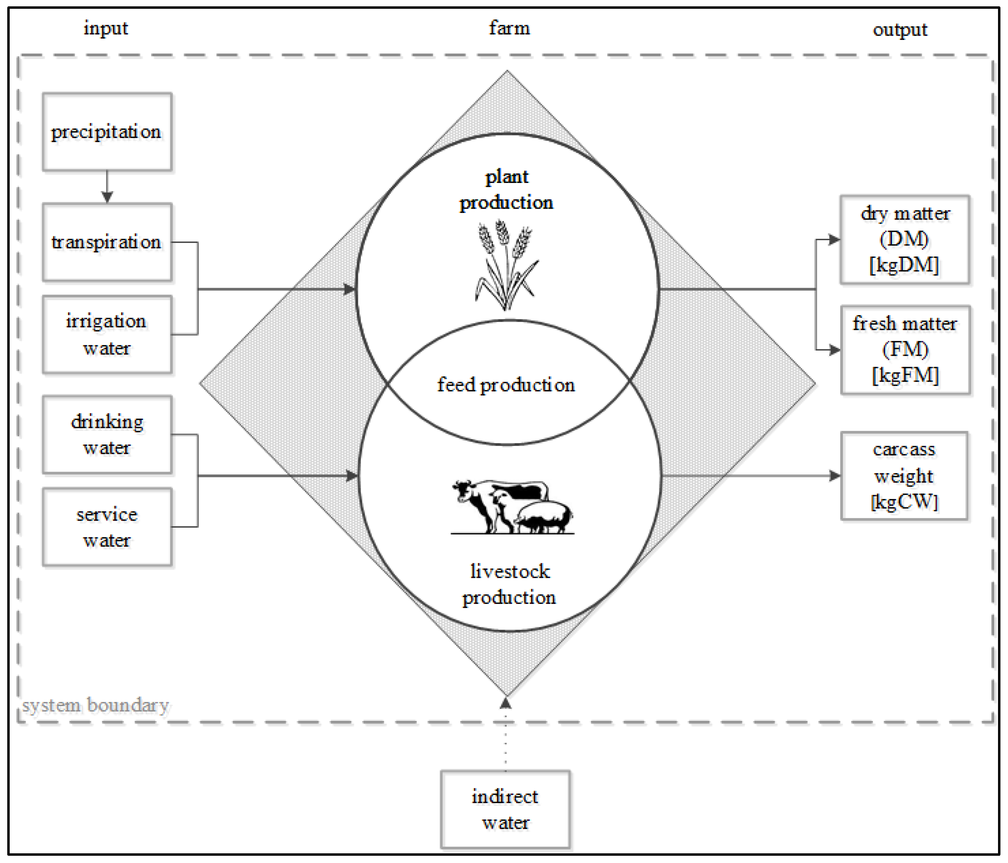
This study analyzed the water productivity for beef production in cow-calf farming systems from cradle-to-farm-gate. The system comprises a defined number of beef cattle and their replacement. The replacements are calves and heifers, which are reared to recreate the dairy herd and to improve the genetics of the herd [38]. The system includes cow specific parameters, such as age at first calving, but also herd specific parameters, such as replacement rate. The replacement rate reflects the ratio of animals coming into the dairy herd to the average herd size [39]. Pre-chains for the production of fertilizer, machines and buildings were excluded as well as transport and processing of livestock products and the water for cleaning, since they were found to be negligible [40,41].

The study considered cow-calf organic farming systems and cow-calf conventional farming systems in north Germany. On the OFS, all beef cattle are born and raised on site.

The spatial boundaries of the system were set from an institutional perspective in the sense that any physical thing that belongs to the farm also belongs to the system (Figure 1) [19]. To obtain the volume of water for purchased feed production, the amount of the feedstuffs purchased from the external suppliers was recorded. Water inflow is, for example, precipitation, which enters through the air and is taken into account in the system after it reaches the plant or soil; surface water and subsurface flows, which enter via the ground, for instance, from areas close to the farm or temporary flooding, or irrigation; tap water, which enters through the plumbing and can be obtained from groundwater or surface water, and which also includes the water used for drinking and cleaning in livestock husbandry; and indirect water, which is used for producing feedstuffs outside the farm, which is then purchased.

2.2.2. Calculation of Indicators

The following indicators were used according to Prochnow et al. [19]:

• Farm water Productivity (FWP)
• Degree of water utilization (DWU)
• Specific technical water inflow (STW)

The Farm water productivity (FWP) was derived from general economic principles and describes the relationship between input and output levels of water in relation to fixed systems. The indicator was used to show weaknesses in production to achieve maximum output with the lowest input [19]. In the case of FWP, the input is water and the output mass of product (on fresh mass base in kg_FM m⁻³W_input or dry mass base in kg_DM m⁻³W_input), food energy or monetary income (€ m⁻³W_input). In this study, energy-base was not considered. Total results of FWP were calculated as weighted average in terms of cultivated area. The farm water productivity was given for the whole farm, for food crops, and for livestock. Farm water productivity of food crops (FWP_{food crops}) were used to examine food crops; farm water productivity of feed crops (FWP_{feed crops}) were used to examine feed crops and farm water productivity livestock (FWP_livestock) were used to examine livestock production.

$${\mathrm{FWP}}_{\mathrm{mass}}=\frac{{\mathrm{Mass}}_{\mathrm{output}}}{{\mathrm{W}}_{\mathrm{input}}}$$

(1)

$${\mathrm{FWP}}_{\mathrm{mon}}=\frac{{\mathrm{Revenues}}_{\mathrm{output}}}{{\mathrm{W}}_{\mathrm{input}}}$$

(2)

The water input (W_input) includes all water which contributes to the generation of output, thus all water which is used for crop growth. It contains water transpired from precipitation (W_prec-transp), all technical (W_tech) and indirect water (W_indirect). All W_tech was considered, because in contrast to W_prec, the farmers have to pay for the entire quantity of water and have to manage it themselves. They are thus responsible for the productivity of this part of water input. W_indirect includes all the water that is used externally for the production of feed as well as the water demand for the construction of machines or of buildings or that is needed to produce energy, fertilizers, pesticides or herbicides. In this paper, this indirect water, except for the off-farm produced feed, was not taken into consideration, since it was assumed to be negligible [20,40,41].

W_input = W_prec-transp + W_tech + W_indirect

(3)

As mentioned above, only transpiration stemming from precipitation contributing to biomass production was considered for calculating the water productivity beside technical water and indirect water. Water evaporating from soil was excluded. This differs from other authors dealing with the virtual water concept, such as water footprint, where generally evapotranspiration from precipitation is included [19]. Evaporation was excluded from W_input, but should be minimized [19].

To characterize the fraction of water which is directly committed to biomass generation, Prochnow et al. [19] introduced the Degree of water utilization (DWU). The DWU shows the relation of productive water W_prod (m³) to the total water inflow W_inflow (m³).

$$\mathrm{DWU}=\frac{{\mathrm{W}}_{\mathrm{prod}}}{{\mathrm{W}}_{\mathrm{inflow}}}$$

(4)

W_prod = W_transp + W_drink + W_feed

(5)

W_inflow = W_prec + W_surf + W_subsurf + W_tech

(6)

The water inflow is the sum of water that enters the system (W_inflow) [m³] via precipitation, surface and subsurface flows or technical water. This includes tap water and irrigation water.

Specific technical water inflow (STW) is composed of irrigation water and further technical water supply such as tap water. This refers to the used technical water per hectare of operating farm area (A_farm)

$$\mathrm{STW}=\frac{{\mathrm{A}}_{\mathrm{farm}}}{{\mathrm{W}}_{\mathrm{tech}}}$$

(7)

W_tech = W_irri + W_tap

(8)

2.3. Calculation of Crop Transpiration

To calculate water flows and water productivity on the farms, crop transpiration was calculated. Therefore, the AgroHyd Farmmodel according to Drastig et al. [14] was used: the model components for the calculation of crop transpiration are based on physically based equations, e.g., the Penman-Monteith equation [42,43]. The AgroHyd Farmmodel takes a variety of input data into account, which range from large datasets on local climate and soils to specific operating data of the investigated farms. The Agrohyd Farmmodel is based on the FAO 56 dual crop coefficient method, according to Allen et al. [40]. Therefore, a reference evapotranspiration (ET₀), the potential crop transpiration (T_c) and the actual transpiration (T_act) from three different datasets climate, plants and soil were calculated. The transpiration of each crop was modeled for the preceding fallow period and for the respective vegetation period.

Thereby climate includes regional climate data of the nearest DWD weather station–temperature, relative humidity, sunshine hours, wind speed, precipitation and global radiation in daily resolution. With these data, ET₀ of a grass reference surface was calculated using the FAO Penman-Monteith equation [22]. T_c was calculated using ET₀ for the individual crop with the plant-specific parameters: crop coefficient, basal crop coefficient, vegetation period, rooting depth, leaf area index, depletion fraction, yield response factor, length of the vegetation period stages, vegetation height. Soil parameters included regional soil data, defined according to official geological soil maps (BÜK 300) or USDA-soil class. Water content at field capacity, water content at wilting point and available water [22] was taken into account.

The water stress coefficient that reduces T_c to T_act was determined through a daily water balance approach combined with regional soil and precipitation data [22]. Therefore, T_act considered the effect of daily water stress, due to water-limited conditions.

As the crop grows, the ground cover, crop height, rooting depth, and the leaf area index changed. Due to differences in transpiration during the various growth stages, the K_cb for a given crop varies over the growing period. The growing period can be divided into four different growth stages: initial, crop development stage, mid-season and late season. The plant-specific parameters for different development stages, basal crop coefficient, leaf area index, rooting depth, average fraction of available soil water, and plant height of each specific crop, were used as parameters in the AgroHyd Farmmodel [20]. The start day and end day describe the length of each of the three development stages.

For the calculation of water flows and water productivity next to transpiration, the amount of irrigation and other tap water was taken into account. Together with farm data such as sowing and harvest date (

Table 1. Date of sowing and harvesting (time period) ¹.

Crop	Sowing Date	Harvest Date
Potato	20 April	15 September
Sown grassland 2	-	-
Oat	7 April	28 July
Winter Rye	10 October	2 August
Summer Rye	12 March	25 July
Spelt	15 October	25 July
Maize	15 April	14 September
Triticale	29 September	7 August
Wheat	17 September	30 July
Rapeseed	28 August	2 August

¹ Varies each year ± 15 days. ² First cutting/consecutive cutting as well as perennial cultivation considered. 2–4 cuts, harvest time varies in every year.

), harvest date of the previous crop or yield, a precise modeling at the scale of the field could be done. For a further and detailed model description, see Drastig et al. [44] and Prochnow et al. [19]. In context, the specific crop yield and the above-mentioned aspects, the specific water use of the single crop and the water productivity could be calculated. In the case of soy, which was mainly imported from Brazil or Argentina, typical Brazilian conditions were assumed for a virtual farm, due to the fact that it was impossible to determine the exact location of the soy farms [19].

2.4. Calculation of Water Demand in Livestock

To calculate water flows and water productivity on the farms, water demand in livestock was calculated. Therefore, the AgroHyd Farmmodel according to Drastig et al. [37] was used. The water demand in livestock includes the drinking and service water, transpired water within the production of feed as well as water stored in feed. The model components for the calculation of water demand in livestock were based on algorithms based on measurements and equations from the literature. Technical water, e.g., as drinking water, was calculated per animal according to [45,46]. This is dependent on the ambient temperature (used in daily resolution) and the weight of the animals [47].

$${\mathrm{W}}_{\mathrm{drink}-\mathrm{cow}}=6.46+0.0728\times {\mathrm{m}}_{\mathrm{b}}$$

(9)

where the daily drinking water intake of cows is W_drink-cow [L d⁻¹], the live weight of the animals m_b.

Service water was taken from farm data; transpired water was calculated as described in Section 2.3; water in feed was calculated based on

Table 2. Dry matter content and average producer prices for crops of OFS and CFS farms.

	Dry Matter Content (% in FM)	Producer Price (€ t−1) OFS	Producer price (€ t−1) CFS
Plant
Potato	23	330	-
Sown Grassland 1	30	56–59	42
Oat	14	380	103
Winter Rye	14	325	98
Summer Rye	14	289	-
Spelt	14	550	-
Maize 1	28	-	46
Triticale	14	-	102
Wheat	14	-	111
Rapeseed	9	-	263

¹ Used as silage.

.

2.5. Farm Data

This study considered three organic farms and two conventional farms with regard to their respective water input for feed production, drinking, cleaning, and cooling (Figure 1). The time frame considered was the period between 2010 and 2015 for crop production. The reference period for the analysis of arable land was calculated at the single field scale from the day after harvesting the preceding main crop and ended with the day of harvest of the main crop in the calendar year being studied [37]. The period of preceding fallows and cover crops were thus included. In the case of animal husbandry, seasonal variations were not necessary due to a smaller annual variation. The reference period was therefore set with the calendar year.

Farm data was collected using a questionnaire in direct personal interviews with the responsible persons during visits to each farm.

Farm 1 (OFS1) and Farm 2 (OFS2) were located in Lower Saxony, having similar structures, and natural conditions. Both farms were located about 70–80 m above sea level in an area that was shaped by the glacial period. Sandy soils predominated with relatively low soil fertility, with soil rating points ranging between 17 and 35 (

Table 3. Site conditions of examined farms.

	Farm 1 (OFS1)	Farm 2 (OFS2)	Farm 3 (OFS3)	Farm 4 (CFS1)	Farm 5 (CFS2)
Federal State	Lower Saxony	Lower Saxony	Brandenburg	Brandenburg	Brandenburg
Temperature (°C)	9.2	9.5	9.2	9.4	9.3
Precipitation (mm)	770	660	521	581	571
Soil	Sandy soil	Sandy soil	Sandy soil	Sandy soil	Sandy soil
Soil Rating Points	17–35	17–35	15–35	15–35	15–35
Size Total Farmland	140	250	500	1000	1083
Type of Farming	OFS: field crops, suckler-cow husbandry	OFS: mixed crops-livestock	OFS: field crop, suckler-cow husbandry	CFS: mixed crops, suckler-cow husbandry	CFS: field crops, suckler-cow husbandry

).

Farm 3 (OFS3), Farm 4 (CFS1), and Farm 5 (CFS2) were located in Brandenburg, embossed through end moraine as well as ground moraine. Hence, the fields were characterized by heterogeneous sandy soil and stones. Soil fertility was also comparatively low, rating points varied between 15 and 35. To calculate the water productivity of the crops and pasture, the data of the nearest German Weather Service (DWD) climate stations were used in daily resolution. The data was provided by the AgroHyd Farmmodel.

The OFS where chosen following certain criteria:

• The three OFS where selected in relation to their location in northern Germany, having comparable site conditions and operational structure (e.g., they cultivated the same crops) in order to give an overview of the water flows and water productivity in organic farming. Two of the three farms keep beef cattle.
• CFS where mainly selected by the criteria that the site conditions fit to the OFS as well as keeping beef cattle in order to give an overview of the differences between organic and conventional farming in beef cattle production.

2.5.1. Data Crop Production

All three OFS operated with a versatile crop rotation with cover crops such as Oil Radish, Serradella, Phacelia, Lupin or Wintercanola. These plants were taken into account in the balance sheet and accounted to the following main crop since it was assumed that they serve as erosion protection as well as humus enrichment and thus improve soil fertility.

In

Table 4. Area on the farms and yields of the individual crops.

	OFS1		OFS2		OFS3		CFS1		CFS2
	Size	Yield	Size	Yield	Size	Yield	Size	Yield	Size	Yield
Area (ha)	62.1	-	51.8	-	130	-	600	-	842	-
Plant Ø yield (tFM)
Potato	12.9	21.4	21.0	25.5	0.5	9.8	-	-	-
Sown grassland	14.9	18.4	10.0	11	11.1	11.8	175	9.2	271	13.2
Oat	12.4	3.5	-	-	54.0	1.0	7.5	1.5	-	-
Winter rye	-	-	14.5	3.1	-	-	142	6.1	-	-
Summer rye	10.8	2.5	-	-	29.7	1.1	-	-	-	-
Spelt	11.0	3.0	6.4	2.5	35.1	1.4	-	-	-	-
Maize	-	-	-	-	-	-	205	32.1	285	30.6
Triticale	-	-	-	-	-	-	71	4.5	-	-
Wheat	-	-	-	-	-	-	-	-	104	4.7
Rapeseed	-	-	-	-	-	-	-	-	182	3.2

the area on the farms are shown in hectare by the individual crop and the average yield. Data of OFS1-3 were collected for the years 2012–2015. For CFS1 data for the years 2011 and 2012 was collected. For CFS2 data for the year 2010 was collected.

Whereas OFS1 and OFS2 used irrigation stemming from groundwater when required, all other farms had no irrigation systems installed. Thus, data on irrigation water withdrawal was collected for OFS1 and OFS1 and considered in the water balancing as water input.

Table 2 shows the moisture content of the crop as well as the producer price, which was used for the calculation of the water productivity on a monetary basis. Conventional producer prices are significantly lower than those of organic farms.

2.5.2. Data Livestock Farming

The number of examined animals and carcass yield of livestock can be seen in

Table 5. Balanced period, number of examined suckler cows.

	OFS1	OFS2	OFS3	CFS1	CFS2
Balanced Period	20 June 2015–19 April 2016	-	20 June 2015–19 April 2016	1 January 2012–31 December 2012	1 January 2010–31 December 2010
Race	Gelbvieh		Gelbvieh	Uckermärker, Simmental	Hybrid (Fleischrind × Fleischrind)
Herd Seize	18	-	30	129	190
CW 1	2436		3480	32,944	52,000
Producer price € kg−1	4.10	-	5.00	2.63	2.63

¹ Ø CW: carcass weight t.

. The drinking water, irrigation water withdrawal and precipitation water which has been transpired in the production of feed, as well as the water stored in feed, were taken into account when balancing the water demand of animal production. To calculate the carcass yield for the calculation of the demand of output, a slaughtering yield of 58% [48,49] was assumed.

On the basis of the diets, the water demand in feed production, and thus also the FWP, was calculated. On the organic farms, two diets were considered to meet the demands of the summer and winter periods because livestock is grazes on pasture during the summertime. Diet components and proportions can be seen in

Table 6. Diet components and proportions of components.

	Diet Components	Diet Proportion Summer (%)	Diet Proportion Winter (%)
OFS1	Grassland Grass silage Hay Potato	95 4 1 -	- 67 30 3
OFS2	-	-	-
OFS3	Hay Straw Grass silage Grassland	- - - 100	24 24 49 3
CFS1	Maize silage Rapeseed meal Soy meal Concentrate Straw	77.84 7.19 3.59 8.38 2.99	See diet proportion summer
CFS2	Grass silage Maize silage Straw Concentrate	34.24 58.7 2.17 4.89

. The daily weight gain according to Rahmann [50] and Golze et al. [51] was used for organic farms and Spiekers et al. [52] for conventional farms. Water use of straw was not accounted for as it is a crop residue. On the OFS all beef cattle are born and raised on site. They are kept as fattening beef cattle with a fattening period of 15–20 months.

Diet components such as soy meal and concentrate, fed on the conventional farms, were not produced on the same farm, thus imported or indirect water was used.

2.6. Comparability of the Farms

Similarities and dissimilarities of the five examined farms are explained in the following. All farms were of the mixed crops—livestock type, according to the Official Journal of the European Union [53]. As shown in Table 3, site conditions were, with respect to mean temperature, soil, and soil rating points, relatively similar. The three farms located in the German federal state of Brandenburg had fewer amounts of yearly precipitation compared to the farms located in the German federal state of Lower Saxony; this could limit comparability concerning the site conditions. Concerning food crop yields, all farms are at the lower end of average yields in Germany, both organic and conventional farms [36], whereas OFS3 has the lowest yields. Thus, the operational structure was well suited for comparison. Regarding the size of the farms, all three farms located in the state of Brandenburg are structurally larger than the two farms located in Lower Saxony with respect to crop production.

On all OFS, beef cattle are kept on grassland during the summer, whereas livestock was in the barns all year on conventional operating farms. As no beef cattle were kept on OFS2, livestock is not considered in this farm.

3. Results

The results of all examined farms are presented as follows: firstly, water flows on the farm scale are pointed out. Secondly, the farm water indicators of plant production, and lastly the water productivity of livestock farming, is shown and compared with the results of plant production.

3.1. Water Flows at Farm Scale

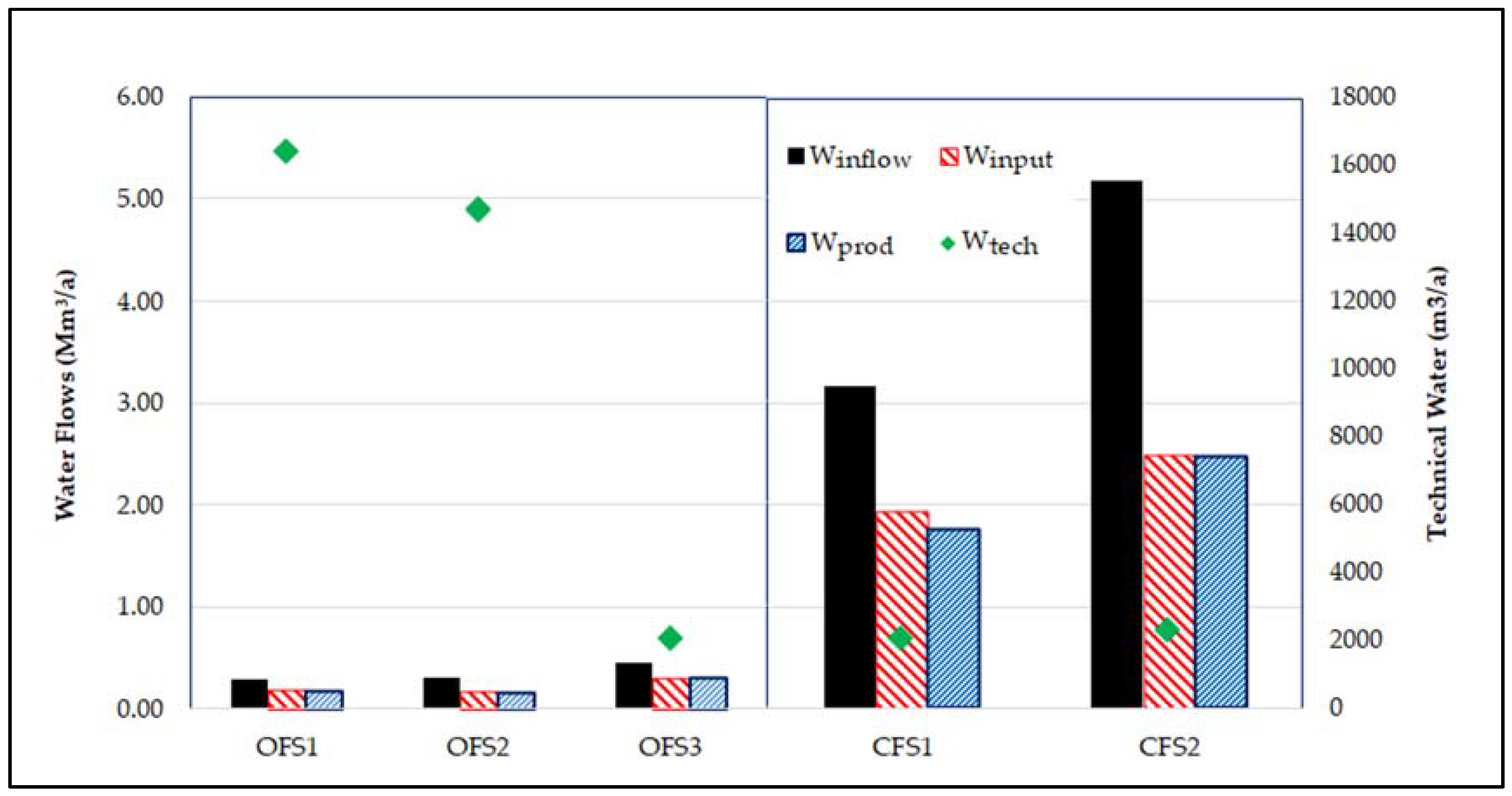
Mean yearly water flows of all examined farms are shown in Figure 2. On farms with irrigation (OFS1, OFS2), precipitation accounts for around 95% of all water inflows. Nearly 5% of water inflow is the result of irrigation. On all other farms without irrigation, precipitation accounts for more than 99% of all water inflows. Tap water in comparison to precipitation is negligible.

The W_input into farms with irrigation (OFS1, OFS2) is composed of around 91% of transpiration from precipitation; on OFS3 (without irrigation) it accounts for 99.9%. On CFS1 and CFS2 indirect water is used through purchased feed (10% of all water input on Farm CFS1 and 1.4% on CFS2 is imported and thus “used” somewhere else). The relation of water input into the farm and all farm water inflows varies between 48% (CFS2) and 66% (OFS3).

Productive water is mainly water transpired by plants (on all farms around 99.7%); around 0.1% is drinking water for animals (except OFS2). Water in product varies, depending on the cultivated crops, between 0.03% (OFS3) and 0.36% (CFS1).

Figure 2 gives an overview on the mean annual water flows of plant production and livestock.

3.2. Farm Water Productivity Food and Feed Crop

The farm water indicators of all examined farms are shown in

Table 7. Farm water productivity food crops (FWP_{food crops}) on a mass basis, monetary basis and farm water productivity feed crops (FWP_{food crops}) on a mass basis using fresh matter (FM). Note: examined crops on farms vary; for detailed comparison, same crops are compared (see Table 8 and Table 9).

	Unit	OFS1	OFS2	OFS3	CFS1	CFS2
FWPfood crops,mass	kgFM m−3Winput	2.40	4.27	0.59	1.14	1.12
FWPfood crops,mon	€m3Winput	0.89	1.44	0.20	0.13	0.22
FWPfeed crops,mass	kgFMm−3Winput	3.73	2.18	3.98	8.60	9.53

. On the following farm, the water productivity of food crop production (FWP_{food crops}) and farm water productivity of feed crop production (FWP_{feed crops}) are used for water productivity of examined crops because they include only parts of the FWP. The highest FWP_{food crops} in FM as well as DM are reached on organic farms (OFS1, OFS2). On the basis of monetary revenues, FWP_{food crops} on organic OFS1 and OFS2 are higher than on CFS1, CFS2, and OFS3. CF1 has the lowest FWP_{food crops} on a monetary basis. On the basis of FWP_{feed crops}, conventional farms show higher water productivity. Nevertheless a comparison between the farms should be made at the level of single crops because the selection of cultivated plants mainly determines the farm water productivity and therefore does not give any indication of the water productivity of the cultivation method (organic or conventional). High yielding crops (maize, potatoes or sown grassland) generally have higher water productivity than crops with lower yield (e.g., spelt, triticale or wheat). Detailed FWP_{food crops} are shown in

Table 8. Farm water productivity of food crops (FWP_{food crops}) on a mass basis, using dry matter (DM) and a monetary basis for the five examined farms. Total values as weighted average by cultivated area.

	Plant	OFS1	OFS2	OFS3	CFS1	CFS2
FWPfood crops,mass [kgDM m−3Winput]	Potato	1.44 1.1 0.9	2.86	1.12	-	-
	Oat	0.92	-	0.57	0.40	-
	Winter Rye	-	1.06	-	1.10	-
	Summer Rye	0.63	-	0.39	-	-
	Spelt	0.86	0.64	0.45	-	-
	Triticale	-	-	-	0.78	-
	Wheat	-	-	-	-	1.19
	Rapeseed	-	-	-	-	0.89
	Crops Total	0.98	1.9	0.49	0.97	1.0
FWPfood crops,mon [€ m−3Winput]	Potato	2.09	2.46	1.16	-	-
	Oat	0.41	-	0.16	0.05	-
	Winter Rye	-	0.4	-	0.15	-
	Summer Rye	0.21	-	0.13	-	-
	Spelt	0.55	0.42	0.29	-	-
	Triticale	-	-	-	0.70	-
	Wheat	-	-	-	-	0.15
	Rapeseed	-	-	-	-	0.26
	Crops Total	0.86	1.44	0.2	0.13	0.22

for the single crops and are discussed later.

As mentioned above, detailed FWP_{food crops} and FWP_{feed crops} are shown in

Table 9. Temperature, precipitation, farm water productivity (FWP) of single food and feed crops in using fresh matter (FM) for examined farms in single year and in total. Total values as weighted average by cultivated area.

		OFS1					OFS2					OFS3					CFS1			CFS2
		2012	2013	2014	2015	Total	2012	2013	2014	2015	Total	2012	2013	2014	2015	Total	2011	2012	Total	2010	Total
Ø Temp. (°C)		9.70	9.40	10.90	10.40	9.20	9.20	9.00	10.60	10.0	9.50	9.70	9.20	9.10	10.4	9.20	10.20	9.60	9.40	8.10	9.30
Ø Prec. (mm)		681	677	639	730	770	697	678	555	711	658	591	543	483	404	525	607	606	581	701	571
FWP Food Crops (kgFM m−3Winput)	Potato	7.53	8.86	4.73	4.0	6.27	7.43	7.79	6.9	7.69	7.45	4.64	4.95	5.07	-	4.89	-			-
	Oat	-	1.30	1.30	0.70	1.10	-	-	-	-	-	-	0.52	0.75	0.71	0.66	0.46	-	0.46	-
	Winter rye	-	-	-	-	-	1.33	1.00	1.38	1.25	1.24	-	-	-	-	-	0.93	1.66	1.29	-
	Summer rye	0.79	0.91	0.76	0.46	0.73	-	-	-	-	-	0.41	0.34	0.59	0.47	0.45	-			-
	Spelt	-	-	-	1.00	1.00	-	0.61	0.48	1.16	0.75	0.46	0.47	0.63	0.55	0.53	-			-
	Triticale	-	-	-	-	-	-	-	-	-	-	-	-	-	-	-	0.88	0.95	0.92	-
	Wheat	-	-	-	-	-	-	-	-	-	-	-	-	-	-	-	-	-	-	1.39
	Rapeseed	-	-	-	-	-	-	-	-	-	-	-	-	-	-	-	-	-	-	0.97
	Food crops Total	4.12	3.70	2.49	1.63	2.40	5.25	4.44	4.18	4.12	4.27	0.47	0.47	0.74	0.57	0.59	0.90	1.37	1.14	1.12
FWP Feed Crops (kgFM m−3Winput)	Sown Grassland	2.13	5.39	5.50	1.89	3.73	2.57	1.64	2.29	2.23	2.18	-	3.46	4.69	3.81	3.98	5.53	6.23	5.60	8.00
	Maize	-	-	-	-	-	-	-	-	-	-	-	-	-	-	-	12.36	7.84	10.1	10.98
	Feed crops Total	2.13	5.39	5.50	1.89	3.73	2.57	1.64	2.29	2.23	2.18	-	3.46	4.69	3.81	3.98	10.31	7.12	8.60	9.53

in FM. For DM and on a monetary basis, see Table 8. The detailed data show that sown grassland clearly has a higher FWP_{food crops} on FM and DM base on conventional farms, whereas there are large differences between the farms: FWP_{food crops} of organic grassland range between 2.18 kg_FM m⁻³W_input and 3.98 kg_FM m⁻³W_input, and on conventional farms between 5.6 kg_FM m⁻³W_input and 8 kg_FM m⁻³W_input.

For winter rye, the comparison of the two cultivation systems shows that the FWP_{food crops} is slightly higher on conventional farms, whereas for oat, the FWP for single crop products is clearly higher on organic farms.

Results show that the differences between organic and conventional agriculture are more pronounced the higher the crop yields of the examined crops are. This also reflects the comparison with the results from Prochnow et al. [20], where the FWP_{food crops} of potatoes, as a high yielding crop, reaches FWP_{food crops}, which is up to twice as high compared to the lowest FWP_{food crops} of potatoes (OFS3) in organic farming, whereas the FWP_{food crops} of winter rye has higher values on organic farms.

On a monetary basis, sown grassland has higher productivity on conventional farms, whereas the differences are less extended compared to the FWP_{food crops} on a mass basis. Oat and winter rye have clearly higher monetary FWP_{food crops} on organic farms.

In Table 9, the temperature and precipitation of the specific examined year as well as the mean average of the farms can be seen. Together with the agricultural meteorology conditions of the year, impacts are discussed later in this paper.

However, it is important to point out that there are large differences in water productivity on organic farms as well as differences on conventional farms, also at the level of the same crops. For example, OFS3 has comparatively low water productivity, except for sown grassland; the water productivity is higher than all other values of organic sown grassland. This makes it difficult to give specific statements on the water productivity of organic or conventional farming in general. Nevertheless, in this study it can be seen that high yielding crops show higher water productivity in conventional farming, whereas considering FWP_{food crops} of grains as lower yielding crops, there is no clear trend to one farming method. Compared to results from Prochnow et al. [20], the same pattern can be seen. There is a trend to higher CWP in conventional farming but this does not apply without exception. On the basis of monetary revenues, the FWP_{food crops} is mainly higher on organic farms—here too, with exceptions. In general, higher selling prices increase the productivity of organic crops.

3.3. Livestock Water Productivity

The WP of the five farming systems are shown in

Table 10. Farm water productivity livestock (FWP_livestock) of the five farming systems using carcass weight (CW), fresh matter (FM) and dry matter (DM).

Indicator	Unit	OFS1	OFS2	OFS3	CFS1	CFS2
Race		Gelbvieh		Gelbvieh	Uckermärker, Simmental	Hybrid (Fleischrind × Fleischrind)
FWPlivestock,mass	kg CW m−3Winput	0.069	-	0.054	0.066	0.090
FWPlivestock,mon	€ m−3Winput	0.283	-	0.269	0.173	0.237

. Farm water productivity of beef cattle production (FWP_livestock) on a mass basis (in carcass weight, CW) varies between 0.09 and 0.05 kgCWm⁻³W_input. The lowest FWP_livestock of beef cattle is reached on organic OFS3 with the Gelbvieh breed; the highest on conventional CFS2 that has the Hybrid breed (Fleischrind × Fleischrind). A plus of 67% compared to OFS3 was found. OFS1 also has the Gelbvieh breed and CFS1 has the Uckermärker breed, Simmental have nearly the same WP in beef cattle production (both around minus 25% compared to CFS2).

On a monetary basis, the FWP_livestock range between 0.17–0.28 € per m³ water input. Thereby FWP_livestock is clearly higher on organic farms (up to plus 63%). Thus, a higher monetary outcome per m³ W_input is reached.

The FWP_livestock in cow-calf farming systems, on a basis of mass compared to the water productivity of crop production, is low. On the farms examined here, on average 0.07 kg CW meat is produced per m³ water input (0.06 kg on organic, 0.08 kg on conventional farms) compared to an average 1.9 kg in crop production (2.42 kg organic and 1.13 kg on conventional farms). This differs from the monetary base, whereas on conventional farms higher monetary revenues from crop production are reached per m³ water input. On organic farms, higher revenues are reached from beef cattle per m³ water input.

3.4. Farm Water Indicators Whole Farm

Farm water indicators are represented in

Table 11. Farm water productivity (FWP_mass) on a mass basis (fresh matter, FM), Degree of water utilization (DWU), and Specific technical water inflow (STW) of the five investigated farms.

	Unit	OFS1	OFS2	OFS3	CFS1	CFS2
FWPmass	kgFM m−3Winput	2.14	-	0.48	0.64	0.45
DWU	-	0.57	0.50	0.66	0.55	0.47
STW	m3 Wtech ha−1 year−1	260.8	276.8	2.40	3.40	2.70

. They consist of FWP (in FM), degree of water utilization (DWU, dimensionless) and specific technical water inflow (STW, m³ per year and ha).

FWP considers crop and beef cattle production of the examined farms, except for OFS2 where livestock has not been examined. FWP clearly shows the highest values on OFS1. As OFS1 has, compared to OFS3, CFS1, and CFS2, a small number of beef cattle, the FWP is not as much affected by the lower water productivity of beef cattle compared to the other farms. Again, a comparison between the farms should be made at the level of single crops or FWP_livestock because the selection of cultivated plants, including or excluding livestock, mainly determines the FWP. The FWP does not allow for a statement about the water productivity of the cultivation method (organic or conventional).

The DWU ranges from 0.47 (CFS2) to 0.66 (OFS3). Thus, OFS3 with comparatively low crop water productivity, has the highest degree of water utilization. These results come from a combination of the rainfall capture efficiency and the soil water use efficiency [19]. Thus, OFS3 has a comparatively low water inflow (precipitation), but the available water is used relatively productively. The DWU value of the farm examined according to Prochnow et al. [19] is 0.56, and thus in the middle of the values of this study.

The STW is the highest on farms with irrigation systems installed (around 270 m³ per year and ha) with respect to farms without an irrigation system (between 2 and 4 m³ per ha and year).

4. Discussion

To enhance productivity and yield stability of organic farming systems, a strategy termed “eco-functional intensification” has been proclaimed by scientists and organic interest groups [3,54,55,56]. This term is loosely based on the paradigm of “sustainable intensification” [57], which is also used by the Food and Agriculture Organization (FAO). In this context, the discourse on water productivity in agricultural production that is aiming at a reduction of water consumption needs to be brought forward. This study seeks to fill the research gap of small-scale considerations on a farm scale, contrasting organic- and conventional agricultural practices.

Findings on water flows, farm water indicators of plant production, livestock and crop water productivity are discussed following the logical structure of Section 3. A methodological discussion pointing out limitations of the study will follow.

Water flows of examined farms give an overview, especially to farmers, of how much and where water is used on their farms. Thereby, the special position of precipitation as W_input as well as irrigation as technical water on farms with installed irrigation system can be seen. The distributions of water flows are similar to the results of [19]. The special position of purchased feed as indirect water used on conventional farms can be seen within the water use in cow-calf farming systems. In particular, the indirect water, which is imported in form of purchased feed, for example soy from Brazil or Argentina and concentrate from different places in Germany, must be underlined. On CFS1 this accounts for around 186,000 m³ or 37.4% (28.3% soy, 9.1% concentrate) of all water transpired in food production. On CFS2 this accounts for 5.4% or nearly 31,000 m³ in the form of concentrate. All three organic farms used no purchased feed within the considered period. However, imported water has unpredictable consequences for the environment and the population in other regions of the world, which must be considered when results are used in impact assessments.

A closer examination of the DWU shows that not the farm with the highest WP has the highest degree of water utilization; it is the farm with the lowest yearly precipitation and also the lowest rates of WP. In the literature, the DWU was calculated from [19] and is similar to the results of this study.

The consideration of the STW shows clearly that the highest technical water per area is used on the two farms with irrigation. Thereby the STW give only the amount of water which is used and no environmental impact of water use.

Regarding FWP_{food crops}, despite small-scale examinations, large differences in the results can be seen, both in the yearly variability within the single farms as well as when comparing the different farms. Looking, for example, at water footprint studies, examinations of total volumes of water used globally or by nation [25,58,59] for crop production are often calculated. Considering the large variation of results of our study, a generic value of water productivity on a farm scale, or even for regions, countries or globally is clearly out of reach.

FWP_{food crops} are closely connected to crop yields. In turn, yields depend on many factors such as specific agro-meteorology, soil fertility, management or, especially in organic agriculture, fungal or insect infestation. For example, on OFS1, FWP_{food crops} of potatoes are relatively low in the years 2014 and 2015. In both years there was a relatively early leaf blight (Phytophthora infestans) with negative effects on yield, and therefore, also on FWP for single crop products. Within this small scale consideration, especially farmers, as they have the whole knowledge about all yield reducing factors, can use the information of water productivity of the single crop and year to reduce water consumption on their farms and in agriculture.

The impact of irrigation, especially using groundwater, is not considered in this study and neither are the negative impacts from intensive livestock husbandry on groundwater bodies and surface water. Regarding the agro-meteorology, it can be assumed that especially spring droughts in recent years were yield-reducing factors, whereas irrigation on OFS1 and OFS2 can be seen as yield guarantees. OFS3, without any irrigation system, has the lowest FWP_{food crops} of all farms and the farm also has the lowest water availability from precipitation (see Table 9). Thus, the farmers on this farm, as well as on CFS1 and CFS2, have no means of responding directing to dryness because no irrigation is used. Nevertheless, the environmental impact, especially of technical water, could be considered, e.g., by using a water scarcity impact assessment such as the AWARE method according to Boulay et al. [60] or the Blue Water Scarcity Index (BWSI) [56].

The greatest potentials to increase water productivity in livestock husbandry are a proliferous feed production and diet selection. On all farms, around 99% of the water used for livestock husbandry is water that has been used for feed production. This correlates to other studies, calculating the WP [13], or water footprint, where around 98% of the total animal footprint comes from their consumed feed [45]. Only approx. 1% consists of technical water. Nevertheless, technical water should not be neglected, due to its special effects, namely, the withdrawal from the environment [19] and its impact. This is an important factor, especially in water scarce ecosystems where the decline of natural water resources eventually reduces the availability of water for terrestrial systems, which consequently affects the diversity of species [40].

The water demand on crop production inputs are not considered in the presented case studies. The management techniques used in OF are considered to be less water consuming than the practices used in CF. The following management practices are used by organic farmers in weed management, pest management, and disease management. Weeds are clearly the biggest problem of OA crop systems. The weed management techniques most commonly used are mechanical cultivation (mechanical tillage, crop rotations, weeding, cover crops). The use of pesticides is minimal—fewer than 10% of OFs use botanical insecticides on a regular basis, 12% use sulfur, and 7% use copper-based compounds. The pest management techniques most commonly used in OA production are crop rotations. Beneficial arthropod and vertebrate habitat, and Bacillus thuringiensis are the most frequently used arthropod pest management strategies. Crop rotations, resistant crop varieties, compost or compost tea applications, Sulfur/sulfur-based materials, copper-based materials, and companion planting were the most commonly cited disease management strategies [1]. Further research on quantifying the water demand on crop production inputs is required.

The results of examined beef cattle cannot be directly compared with the results from Prochnow et al. [20] because in that study water flows and FWP of dairy cows, veal calves and heifers were examined together. Nevertheless, it can be shown that FWP is significantly higher with the inclusion of milk as a product (the FWP for livestock in that case study is 1.32 kg_FM m⁻³W_input). Palhares et al. [5] examined the water footprint of organic and conventional dairy production systems. Thereby an equal green water scarcity was calculated for organic and conventional agriculture and a lower blue water scarcity for conventional farming was calculated, concluding that a product with a lower water footprint could be more damaging to the environment than one with a higher water footprint, depending on water availability. The examination of FWP in cow-calf farming systems shows a similar picture to FWP_{food crops} where the highest farm water productivity on a mass basis occurs on a conventional farm, whereas the second conventional farm has values comparable to examined organic farms. Due to higher selling prices, FWP_{food crops} on a monetary basis are significantly higher on organic farms.

Both the results of this paper and the methodology used are difficult to compare to other authors’ works: different scales are used (e.g., the water footprint concept or life cycle assessments consider the product scale) as well as different basic assumptions, as e.g., a different handling of transpiration and evapotranspiration as well as taking water withdrawal as irrigation water into account. Other farms examined according to the method of Prochnow et al. [19] consider different agricultural branches such as broiler production [20], wine production [22] or milk production [57] and are therefore not suitable for a comparison with this study.

As mentioned earlier, organic agriculture distinguishes itself in various aspects from conventional agriculture: e.g., the sustainable improvement of soil fertility and the humus accumulation in organic agriculture, which leads to a higher water holding capacity and, especially during droughts, ensures yields [9]. Within this study, this aspect could not be demonstrated, due to the short period examined. However, further investigations in long-term studies under, using the AgroHyd Farmmodel, could illustrate the differences between organic and conventional farming, due to the small-scale examination of farms.

Methodological Discussion

This study presents the first farm water productivity calculation in organic farming in Germany. The method has been used for calculating FWP on several farms with different investigation topics. In general, it is difficult to find similar organic and conventional farms which can be compared in any operational direction. In the best case, various farms should be found with the same crop rotation and same livestock husbandry within the same region and same site conditions.

Environmental impacts of production are not yet involved within the method of Prochnow et al. [19]. Environmental impacts of agriculture have many different levels, such as e.g., biodiversity, eutrophication, nitrogen or nitrate leaching, nitrous oxide or ammonia emissions, to name just a few. As organic farming practice has generally positive impacts on the environment per unit of area, but not necessarily per unit of product [61], environmental impacts of farms should be considered on a farm scale. Within a region characterized by intensive agriculture, the benefits of organic farming can significantly differ from the environmental impact within extensively used agro-ecosystems. Therefore, an indicator which considers the environmental impact and the benefits of the specific cultivation method should be added.

In this study, water use and hydrological information is generally estimated/modelled for all scales of assessments; this results in data uncertainty [61,62]. Hence, a tiered approach of uncertainty assessment should be made to give information about data accuracy of the investigation. Thereby, this study reaches tier level 3 with the highest spatial and temporal scale as well as data sources. Nevertheless, there are several aspects which limit the accuracy of these models:

• Growth rate of beef cattle were estimated in daily rates according to values from the literature, since not the entire stock could be weighed. Livestock generally does not grow homogeneously, whereas in this case this was assumed to reduce complexity.
• During the modeling, a fixed date has to be defined for seed date as well as harvest date to calculate the precipitation and transpiration rate of the main crop. In practice, harvests of, e.g., potatoes do not take place in one day. Therefore, the middle date of harvest of the main crop was estimated.

5. Conclusions

Water flows and water productivity of crop and beef cattle production of different cultivation methods were examined and determined within this study on a farm scale. The results can reveal possibilities to farmers on how to optimize the water productivity on their farms.

Due to large differences within water productivity of different cultivation methods, no generalized statement can be made about the more proliferous cultivation method in crop production in Germany. Nevertheless, results show that higher mass farm water productivity can be achieved in conventional farming within higher yielding crops, whereas lower yielding crops are in some cases associated with higher farm water productivity in organic farming. On a monetary basis, mainly organic farms reach a higher income per m³ water input; here, too, with exceptions. The same applies to beef cattle production on a mass basis. There are great differences in farm water productivity, whereas the highest farm water productivity can be found in conventional farming, the lowest in organic farming. One conventional farm and one organic farm reach almost the same values. On a monetary basis, the highest water productivity is reached on organic farms.

Results show that even with a precise examination of water productivity on a farm scale, a high bandwidth of values are revealed on different farms, although some of the farms have similar natural and operating conditions: generic FWP for food crops and livestock are not within reach.

Additional support for water footprint management policies in the farming through using sustainable practices for water footprint mitigation present [63]. Future research is required for the building up of a database of water indicators from farms using different management practices (including different crop varieties) for specific regions. The evaluation of differences in water productivity between different farm systems can be achieved through this. The main research topics in OFS are: organic plant breeding, site-specific tillage practices and crop patterns, cropping strategies for leguminous crops etc. [64].

Examined organic farms use no purchased feed within their diet in cattle production, whereas the two conventional farms do. Especially CFS2 uses soy from Brazil or Argentine and thus not only shifts possible water use but also environmental impacts to other regions in the world.

In general, the method shows a high accuracy, due to the collection of data on a farm level. This gives a high resolution in terms of the water which is used in the production of crops and beef.

The main goal of organic farming is the sustainable cultivation of the land and a focus on soil and water protection as well as species and animal protection. Therefore, high water productivity in organic agricultural production is also a priority target as is the environmental effect of the farm. This study shows the water productivity performance of three organic farms and two conventional farms in crop and beef cattle production in Germany.

So far, environmental impacts are not considered within the applied method. Since environmental impact can vary from region to region, and from farm to farm, an indicator that takes into account major environmental impacts should be applied on a farm level.

References

- BMEL. Biologischer Landbau. Available online: https://www.bmel.de/DE/Landwirtschaft/Nachhaltige-Landnutzung/Oekolandbau/_Texte/OekologischerLandbauDeutschland.html (accessed on 10 July 2018).
- Lotter, D.W. Organic agriculture. J. Sustain. Agric. 2003, 21, 59–128. [Google Scholar] [CrossRef]
- Siegmeier, T.; Blumenstein, B.; Möller, D. Farm biogas production in organic agriculture: System implications. Agric. Syst. 2015, 139, 196–209. [Google Scholar] [CrossRef]
- Stolze, M. The Environmental Impacts of Organic Farming in Europe; Inst. für Landwirtschaftliche Betriebslehre: Stuttgart-Hohenheim, Germany, 2000; p. 127. [Google Scholar]
- Palhares, J.C.P.; Pezzopane, J.R.M. Water footprint accounting and scarcity indicators of conventional and organic dairy production systems. J. Clean. Prod. 2015, 93, 299–307. [Google Scholar] [CrossRef]
- Dormaar, J.; Lindwall, C.; Kozub, G. Effectiveness of manure and commercial fertilizer in restoring productivity of an artificially eroded Dark Brown Chernozemic soil under dryland conditions. Can. J. Soil Sci. 1988, 68, 669–679. [Google Scholar] [CrossRef]
- Stanhill, G. The comparative productivity of organic agriculture. Agric. Ecosyst. Environ. 1990, 30, 1–26. [Google Scholar] [CrossRef]
- Sylvia, D.M.; Williams, S.E. Vesicular-arbuscular mycorrhizae and environmental stress. Mycorrhizae Sustain. Agric. 1992, 54, 101–124. [Google Scholar]
- Gomiero, T.; Pimentel, D.; Paoletti, M.G. Environmental Impact of Different Agricultural Management Practices: Conventional vs. Organic Agriculture. Crit. Rev. Plant Sci. 2011, 30, 95–124. [Google Scholar] [CrossRef]
- Li, S.-X.; Wang, Z.-H.; Malhi, S.S.; Li, S.-Q.; Gao, Y.-J.; Tian, X.-H. Nutrient and Water Management Effects on crop Production, and Nutrient and Water use Efficiency in Dryland Areas of China. In Advances in Agronomy; Academic Press: Cambridge, MA, USA, 2009; pp. 223–265. [Google Scholar]
- Withers, B.; Vipomd, S.; Lecher, K. Bewässerung; Paul Parey: Berlin, Germany, 1978. [Google Scholar]
- Drastig, K.; Prochnow, A.; Baumecker, M.; Berg, W.; Brunsch, R. Agricultural water management in Brandenburg. DIE ERDE–J. Geogr. Soc. Berl. 2011, 142, 119–140. [Google Scholar]
- Fusco, G.; Miglietta, P.P.; Porrini, D. How Drought Affects Agricultural Insurance Policies: The Case of Italy. J. Sustain. Dev. 2018, 11, 1. [Google Scholar] [CrossRef]
- DWD. Zahlen und Fakten zum Klima in Deutschland. Available online: https://www.dwd.de/DE/presse/pressekonferenzen/DE/2015/PK_10_03-2015/zundf_zur_pk.pdf;jsessionid=723D4B00CF437C727093ABB3C2651437.live21074?__blob=publicationFile&v=3 (accessed on 10 July 2018).
- Trömel, S.; Schönwiese, C.D. Robust trend estimation of observed German precipitation. Theor. Appl. Climatol. 2008, 93, 107–115. [Google Scholar] [CrossRef]
- Schönwiese, C.; Janoschitz, R. Klimatrendatlas Deutschland 1901–2000 [The Climate Trend Atlas Germany 1901–2000]; Institut für Atmosphäre und Umwelt: Frankfurt, Germany, 2008. [Google Scholar]
- Drastig, K.; Prochnow, A.; Libra, J.; Koch, H.; Rolinski, S. Irrigation water demand of selected agricultural crops in Germany between 1902 and 2010. Sci. Total Environ. 2016, 569–570, 1299–1314. [Google Scholar] [CrossRef] [PubMed]
- Köstner, B.; Surke, M.; Bernhofer, C. Klimadiagnose der Region Berlin/Barnim/Uckermark/Uecker-Randow für den Zeitraum 1951 bis 2006.-Materials of the Interdisciplinary Research Group, Options for a Future-Oriented Land-Use of Rural Areas; IAG Landinnovation Berlin Brandenburg Academy of Sciences and Humanities: Berlin, Germany, 2007; p. 51. [Google Scholar]
- Prochnow, A.; Drastig, K.; Klauss, H.; Berg, W. Water use indicators at farm scale: Methodology and case study. Food Energy Secur. 2012, 1, 29–46. [Google Scholar] [CrossRef]
- Drastig, K.; Palhares, J.C.P.; Karbach, K.; Prochnow, A. Farm water productivity in broiler production: Case studies in Brazil. J. Clean. Prod. 2016, 135, 9–19. [Google Scholar] [CrossRef]
- Krauss, M.; Keßler, J.; Prochnow, A.; Kraatz, S.; Drastig, K. Water productivity of poultry production: The influence of different broiler fattening systems. Food Energy Secur. 2015, 4, 76–85. [Google Scholar] [CrossRef]
- Peth, D.; Drastig, K.; Prochnow, A. Quantity-and quality-based farm water productivity in wine production: Case studies in Germany. Water 2017, 9, 88. [Google Scholar] [CrossRef]
- ISO. ISO 14046: Environmental Management, Water Footprint—Principles, Requirements and Guidelines; ISO: Geneva, Switzerland, 2014; p. 72. [Google Scholar]
- Garrido, A.; Llamas, M.R.; Varela-Ortega, C.; Novo, P.; Rodríguez-Casado, R.; Aldaya, M.M. Water Footprint and Virtual Water Trade in Spain: Policy Implications; Springer Science & Business Media: Berlin/Heidelberg, Germany, 2010; Volume 35. [Google Scholar]
- Hoekstra, A.Y.; Mekonnen, M.M.; Chapagain, A.K.; Mathews, R.E.; Richter, B.D. Global monthly water scarcity: Blue water footprints versus blue water availability. PLoS ONE 2012, 7, e32688. [Google Scholar] [CrossRef] [PubMed]
- Miglietta, P.P.; De Leo, F.; Ruberti, M.; Massari, S. Mealworms for food: A water footprint perspective. Water 2015, 7, 6190–6203. [Google Scholar] [CrossRef]
- Miglietta, P.P.; Morrone, D.; Lamastra, L. Water footprint and economic water productivity of Italian wines with appellation of origin: Managing sustainability through an integrated approach. Sci. Total Environ. 2018, 633, 1280–1286. [Google Scholar] [CrossRef] [PubMed]
- Owusu-Sekyere, E.; Jordaan, H.; Chouchane, H. Evaluation of water footprint and economic water productivities of dairy products of South Africa. Ecol. Indic. 2017, 83, 32–40. [Google Scholar] [CrossRef]
- Allan, J.A. Fortunately there are substitutes for water otherwise our hydro-political futures would be impossible. Prior. Water Resour. Alloc. Manag. 1993, 13, 26. [Google Scholar]
- ISO. ISO 14040: Environmental Management-Life Cycle Assessment-Principles and Framework; International Organization for Standardization (ISO): Geneva, Switzerland, 2006; p. 20. [Google Scholar]
- ISO. ISO 14044: Environmental Management-Life Cycle Assessment-Requirements and Guidelines; International Organization for Standard (ISO): Geneva, Switzerland, 2006; p. 46. [Google Scholar]
- Descheemaeker, K.; Amede, T.; Haileslassie, A. Livestock and Water Interactions in Mixed Crop-Livestock Farming Systems of Sub-Saharan Africa: Interventions for Improved Productivity; IWMI: Colombo, Sri Lanka, 2009. [Google Scholar]
- Haileslassie, A.; Peden, D.; Gebreselassie, S.; Amede, T.; Descheemaeker, K. Livestock water productivity in mixed crop–livestock farming systems of the blue nile basin: Assessing variability and prospects for improvement. Agric. Syst. 2009, 102, 33–40. [Google Scholar] [CrossRef]
- Kebebe, E.; Oosting, S.; Haileslassie, A.; Duncan, A.; de Boer, I. Strategies for improving water use efficiency of livestock production in rain-fed systems. Animal 2015, 9, 908–916. [Google Scholar] [CrossRef] [PubMed]
- Molden, D.; Oweis, T.; Steduto, P.; Bindraban, P.; Hanjra, M.A.; Kijne, J. Improving agricultural water productivity: Between optimism and caution. Agric. Water Manag. 2010, 97, 528–535. [Google Scholar] [CrossRef]
- Rockström, J.; Karlberg, L.; Wani, S.P.; Barron, J.; Hatibu, N.; Oweis, T.; Bruggeman, A.; Farahani, J.; Qiang, Z. Managing water in rainfed agriculture—The need for a paradigm shift. Agric. Water Manag. 2010, 97, 543–550. [Google Scholar] [CrossRef]
- Drastig, K.; Kraatz, S.; Libra, J.; Prochnow, A.; Hunstock, U. Implementation of hydrological processes and agricultural management options into the ATB-modeling database to improve the water productivity at farm scale. Agron. Res 2013, 11, 31–38. [Google Scholar]
- Thornton, P.K. Livestock production: Recent trends, future prospects. Philos. Trans. R. Soc. B 2010, 365, 2853–2867. [Google Scholar] [CrossRef] [PubMed]
- Kraatz, S. Energy intensity in livestock operations–modeling of dairy farming systems in Germany. Agric. Syst. 2012, 110, 90–106. [Google Scholar] [CrossRef]
- De Boer, I.J.; Hoving, I.E.; Vellinga, T.V.; Van de Ven, G.W.; Leffelaar, P.A.; Gerber, P.J. Assessing environmental impacts associated with freshwater consumption along the life cycle of animal products: The case of Dutch milk production in Noord-Brabant. Int. J. Life Cycle Assess. 2013, 18, 193–203. [Google Scholar] [CrossRef]
- Döring, K.; Kraatz, S.; Prochnow, A.; Drastig, K. Indirect water demand of dairy farm buildings. Agric. Eng. Int. CIGR J. 2013, 15, 16–22. [Google Scholar]
- Allen, R.G.; Pereira, L.S.; Raes, D.; Smith, M. Crop Evapotranspiration: Guidelines for Computing Crop Water Requirements; FAO Irrigation and Drainage Paper 56; FAO: Rome, Italy, 1998. [Google Scholar]
- Monteith, J.L. Evaporation and environment. Symp. Soc. Exp. Biol. 1965, 19, 205–234. [Google Scholar] [PubMed]
- Drastig, K.; Prochnow, A.; Kraatz, S.; Libra, J.; Krauß, M.; Döring, K.; Müller, D.; Hunstock, U. Modeling the water demand on farms. Adv. Geosci. 2012, 32, 9–13. [Google Scholar] [CrossRef] [Green Version]
- Krauss, M.; Drastig, K.; Prochnow, A.; Rose-Meierhofer, S.; Kraatz, S. Drinking and cleaning water use in a dairy cow barn. Water 2016, 8, 302. [Google Scholar] [CrossRef]
- Meyer, U.; Everinghoff, M.; Gädeken, D.; Flachowsky, G. Investigations on the water intake of lactating dairy cows. Livest. Prod. Sci. 2004, 90, 117–121. [Google Scholar] [CrossRef]
- KTBL. Wasserversorgung in der Rinderhaltung: Wasserbedarf-Technik-Management; Kuratorium für Technik und Bauwesen in der Landwirtschaft (KTBL): Frankfurt, Germany, 2008; p. 60. [Google Scholar]
- Geuder, U.; Pickl, M.; Scheidler, M.; Schuster, M.; Götz, K. Mast-, Schlachtleistung und Fleischqualität bayerischer Rinderrassen. Zuechtungskunde 2012, 84, 485–499. [Google Scholar]
- Omlor, M. Schlachtausbeute B1 Schlachttiere; BLE: Berlin, Germany, 2010; p. 10. [Google Scholar]
- Rahmann, G. Ökologische Tierhaltung: 63 Tabellen; Ulmer: Stuttgart, Germany, 2004; p. 136. [Google Scholar]
- Golze, M.; Balliet, U.; Balitzer, J.; Görner, C.; Pohl, G.; Stockinger, C.; Triphaus, H.; Zens, J. Extensive Rinderhaltung. Fleischrinder–Mutterkühe, Rassen, Herdenmanagement, Wirtschaftlichkeit; BLV Verlagsgesellschaft mbH: München, Germany, 1997; p. 159. [Google Scholar]
- Spiekers, H.; Nußbaum, H.; Potthast, V. Erfolgreiche Milchviehfütterung:[mit Futterkonservierung]; DLG Verlag: Frankfurt, Germany, 2009; p. 576. [Google Scholar]
- EU. Regulations Commission Delegated Regulation (EU) no 1198/2014 of 1 August 2014 Supplementing Council Regulation (EC) no 1217/2009. Available online: https://eur-lex.europa.eu/legal-content/EN/TXT/PDF/?uri=CELEX:32014R1198&from=en (accessed on 10 July 2018).
- Niggli, U.; Slabe, A.; Schmid, O.; Halberg, N.; Schlüter, M. Vision for an Organic Food and Farming Research Agenda 2025. Organic Knowledge for the Future. 2008. Available online: http://orgprints.org/13439/1/niggli-etal-2008-technology-platform-organics.pdf (accessed on 10 July 2018).
- Rahmann, G.; Oppermann, R.; Paulsen, H.M.; Weißmann, F. Good, but not good enough? Research and development needs in organic farming. Landbauforsch 2009, 59, 29–40. [Google Scholar]
- Schmid, O.; Padel, S.; Halberg, N.; Huber, M.; Darnhofer, I.; Micheloni, C.; Koopmans, C.; Bügel, S.; Stopes, C.; Willer, H. Strategic Research Agenda for Organic Food and Farming; TP Organics: Brussels, Belgium, 2009. [Google Scholar]
- Pretty, J.N.; Noble, A.D.; Bossio, D.; Dixon, J.; Hine, R.E.; Penning de Vries, F.W.; Morison, J.I. Resource-conserving agriculture increases yields in developing countries. Environ. Sci. Technol. 2006, 40, 1114–1119. [Google Scholar] [CrossRef] [PubMed]
- Hoekstra, A.Y.; Chapagain, A.K.; Aldaya, M.M.; Mekonnen, M.M. The Water Footprint Assessment Manual: Setting the Global Standard; Taylor & Francis: London, UK; Washington, DC, USA, 2009; p. 203. [Google Scholar]
- Mekonnen, M.M.; Hoekstra, A.Y. The green, blue and grey water footprint of crops and derived crop products. Hydrol. Earth Syst. Sci. 2011, 15, 1577–1600. [Google Scholar] [CrossRef] [Green Version]
- Boulay, A.-M.; Bare, J.; Benini, L.; Berger, M.; Lathuillière, M.J.; Manzardo, A.; Margni, M.; Motoshita, M.; Núñez, M.; Pastor, A.V.; et al. The WULCA consensus characterization model for water scarcity footprints: Assessing impacts of water consumption based on available water remaining (AWARE). Int. J. LCA 2018, 23, 368–378. [Google Scholar] [CrossRef]
- Tuomisto, H.L.; Hodge, I.D.; Riordan, P.; Macdonald, D.W. Does organic farming reduce environmental impacts? —A meta-analysis of European research. J. Environ. Manag. 2012, 112, 309–320. [Google Scholar] [CrossRef] [PubMed]
- Goedkoop, M.; Oele, M.; Leijting, J.; Ponsioen, T.; Meijer, E. Introduction to LCA with SimaPro. Available online: https://www.pre-sustainability.com/download/SimaPro8IntroductionToLCA.pdf (accessed on 10 July 2018).
- Aivazidou, E.; Tsolakis, N.; Iakovou, E.; Vlachos, D. The emerging role of water footprint in supply chain management: A critical literature synthesis and a hierarchical decision-making framework. J. Clean. Prod. 2016, 137, 1018–1037. [Google Scholar] [CrossRef]
- BÖLW. Forschungsfragen aus der Praxis: Woran muss Geforscht Werden, um die Ökologische Lebensmittelwirtschaft weiter Voranzubringen? Available online: https://www.boelw.de/themen/wissenstransfer/forschungsbedarf/ (accessed on 10 July 2018).
Figure 1.
System boundaries following [33], adapted.
Figure 2.
Mean annual water flows (2012–2015) of plant production and livestock at, left panel: three organic farms; right panel: two conventional farms. OFS2 without livestock farming.