Communication

Considering a Threshold Energy in Reactive Transport Modeling of Microbially Mediated Redox Reactions in an Arsenic-Affected Aquifer

1
Department of Earth and Environmental Sciences, University of Milano-Bicocca, Piazza della Scienza 1, 20126 Milan, Italy
2
Geological Survey of Denmark and Greenland, Øster Voldgade 10, 1350 Copenhagen, Denmark
*
Author to whom correspondence should be addressed.
Water 2018, 10(1), 90; https://doi.org/10.3390/w10010090
Submission received: 14 November 2017 / Revised: 12 January 2018 / Accepted: 19 January 2018 / Published: 20 January 2018
(This article belongs to the Special Issue Heavy Metals and Potentially Toxic Elements (PTEs) in Water)

Abstract

:
The reductive dissolution of Fe-oxide driven by organic matter oxidation is the primary mechanism accepted for As mobilization in several alluvial aquifers. These processes are often mediated by microorganisms that require a minimum Gibbs energy available to conduct the reaction in order to sustain their life functions. Implementing this threshold energy in reactive transport modeling is rarely used in the existing literature. This work presents a 1D reactive transport modeling of As mobilization by the reductive dissolution of Fe-oxide and subsequent immobilization by co-precipitation in iron sulfides considering a threshold energy for the following terminal electron accepting processes: (a) Fe-oxide reduction, (b) sulfate reduction, and (c) methanogenesis. The model is then extended by implementing a threshold energy on both reaction directions for the redox reaction pairs Fe(III) reduction/Fe(II) oxidation and methanogenesis/methane oxidation. The optimal threshold energy fitted in 4.50, 3.76, and 1.60 kJ/mol e for sulfate reduction, Fe(III) reduction/Fe(II) oxidation, and methanogenesis/methane oxidation, respectively. The use of models implementing bidirectional threshold energy is needed when a redox reaction pair can be transported between domains with different redox potentials. This may often occur in 2D or 3D simulations.

1. Introduction

Arsenic pollution of groundwater is a well-known environmental problem that affects millions of people worldwide [1]. In most cases, the origin of As pollution is related to natural processes occurring in the aquifer system. One of the mechanisms accepted for As release in several alluvial aquifers worldwide is the reductive dissolution of Fe-oxides containing As driven by organic matter (OM) oxidation [1,2]. The OM driving As release can have different sources that could be anthropogenic, e.g., hydrocarbons plumes [3], or natural, e.g., sedimentary (such as peat layers [4,5]) or surface derived OM [6]. Although in some cases (as for South and South East Asia) the identification of the source of OM remains controversial [6,7,8], in other cases, a relative consensus is reached, as for the sedimentary basin of Po Plain (N Italy), where many authors identified peat layers as the source of OM driving As release [9,10,11,12,13]. Beyond the source of OM, what is largely accepted is that the degradation of OM and the reductive dissolution of Fe-oxide, together with other terminal electron accepting processes (TEAPs), are mediated by bacteria [14,15,16,17]. Therefore, microbial activity has a primary role in the processes governing As mobility, so that some treatments for the removal of As from water are based on microbial processes [18,19], in particular, bacteria isolated from natural aquifer systems, such as those belonging to Rhodococcus sp., Achromobacter sp., and Aliihoeflea sp. [19], which have shown good efficiency in As removal processes. Microbes mediate TEAP reactions to obtain energy. The energy is conserved in the form of adenosine triphosphate (ATP), which requires a certain energy to be activated. The stored energy is used for cell maintenance and growth, and biomass synthesis, etc. [20,21,22]. It follows that bacteria are only liable to conduct a TEAP reaction if a minimum Gibbs energy is overcome.
In the last decades, some research efforts were devoted to developing a quantitative understanding of the processes governing As mobility through the implementation of reactive transport modeling [11,23,24,25,26,27]. However, none of these previous modeling efforts implemented the role of bacteria in mediating OM degradation and related TEAPs within the numerical simulations of As mobility. Only a few studies considered the role of bacteria in mediating reactions in reactive transport modeling [28,29,30], through the implementation of a threshold energy for the occurrence of TEAPs [28,29]. This threshold energy represents the minimum Gibbs energy required by bacteria to conduct the reaction [31,32], in order to sustain their life functions. Jakobsen and Cold [29] considered a threshold energy for TEAPs in unidirectional reactions, whereas Jakobsen [28] improved this approach by implementing a threshold energy on both reaction direction for the redox reaction pair methanogenesis/methane oxidation.
This work presents the reactive transport modeling of an aquifer system where As is released by the reductive dissolution of Fe-oxide and attenuated by the co-precipitation in iron sulfide considering a threshold energy for the occurrence of the following TEAPs: (a) Fe-oxide reduction, (b) sulfate reduction, and (c) methanogenesis. This is an improvement of the previous modeling done by Rotiroti et al. [11], where no bioenergetics were implemented. The aim of the present work is to provide a better and more reliable modeling of reduction processes governing As mobility through the implementation of the role played by bacteria in mediating TEAP reactions. Indeed, imposing a threshold energy for the occurrence of Fe-oxide, sulfate reduction, and methanogenesis that drive As release and attenuate it and sustain its release in the studied aquifer, implies, indirectly, that more constraints are applied to the modeling of As mobility. This may lead to a better understanding of the hydro-bio-geochemistry of the aquifer system under analysis. A focus is given to the modeling of Fe-oxide reduction, since it leads to the release of As in groundwater, through the implementation of a threshold energy for both reaction directions for the redox pair Fe(III) reduction/Fe(II) oxidation. To the best of our knowledge, this is the first time that a bidirectional threshold energy for the Fe(III)/Fe(II) redox pair has been used in reactive transport modeling. Furthermore, a bidirectional threshold energy was also implemented for the redox pair methanogenesis/methane oxidation.

2. Materials and Methods

2.1. Study Area

This work refers to the study area of ~150 km2 around the town of Cremona in the Po Plain of N Italy, between longitudes 569,420.6 and 587,240.8 E and latitudes 4,991,333.9 and 5,004,382.3 N (UTM 32 zone 32 N), which was described in detail by previous studies [11,12,33,34], so only a brief summary is given here. The subsurface hosts a multilayer aquifer system constituted by a vertical alternation of sands (i.e., aquifers) with silty clays (i.e., aquitards) that frequently include peat deposits. Within the first 260 m of depth, the system hosts five aquifer units: aquifers U (unconfined, 0–25 m bgl); S (semi-confined, 3–50 m bgl); C1 (confined, 6–85 m bgl); C2 (confined, 10–150 m bgl); and C3 (confined, 16–260 m bgl). Groundwater in shallow aquifers (U and S) mainly flows from N to S, whereas in the deeper confined aquifers (C1, C2, C3), it flows from NW to SE. A component of downward groundwater flow is observed from aquifer U to C2, whereas the flow is directed upwards from C3 to C2. Concerning hydrochemistry, aquifer U has redox conditions that change from oxidizing to reducing in response to local factors, whereas all the other aquifers are anoxic with concentrations of As, Fe, Mn, and NH4 that frequently exceed the regulatory limits (i.e., 10, 200, 50, and 500 µg/L, respectively).

2.2. Hydrogeochemical Conceptual Model

The conceptual model for aquifer hydrogeochemistry of the study area was developed in previous studies [11,12,34], and a brief summary is given below. The aquifer system under analysis is characterized by reducing conditions that are favored by (a) longer groundwater circulation for the deeper confined aquifers [34] and the presence of shallow silty-clay layers capping the shallow aquifers [12] that limit the aquifer recharge by oxygenated waters; and (b) the diffuse presence of peat deposits within silty-clay layers [11] that, when degrading, leads to oxygen consumption, followed by the sequence of TEAPs. There is a tendency toward more reduced conditions over depth.
The high As concentrations found (<183 µg/L) are due to the reductive dissolution of Fe-oxides coupled to the degradation of OM sourced from peat deposits. The peak of As concentrations is attained in intermediate aquifers (~50–100 m bgl) since here the Fe-oxide reduction reaches an advanced stage [12,35]. At increasing depths, the As concentrations are attenuated by the co-precipitation into iron sulfides formed by the products of Fe-oxide and sulfate reduction [11,36,37]. More specifically, the As release and attenuation in the studied system is governed by the Fe-oxide reduction, sulfate reduction, and iron sulfide precipitation that likely occur close to a simultaneous equilibrium [11]. Dissolved Fe in the system is governed by the above mentioned simultaneous equilibrium and by siderite precipitation [11]. Dissolved Mn is governed by Mn-oxide reduction, which does not appear to occur near equilibrium, and by rhodochrosite precipitation close to equilibrium [11].

2.3. Modeling Strategy

This work presents reactive transport modeling with increasing degrees of complexity following a stepwise modeling approach. Four models were implemented:
  • Model 0—this model had no threshold energy for TEAPs and the simpler “partial equilibrium” approach [38] is used; this is the model presented in the previous work by Rotiroti et al. [11].
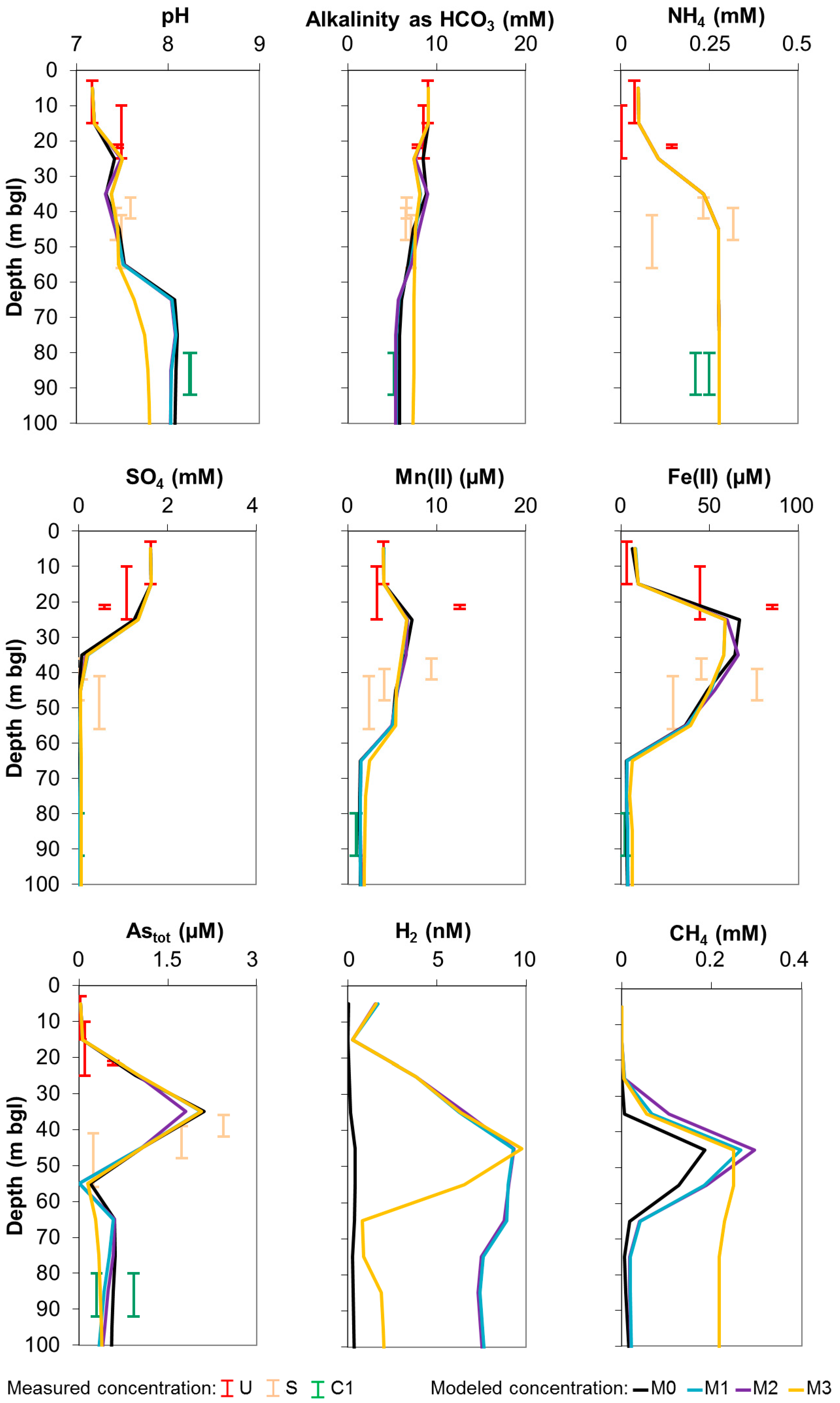
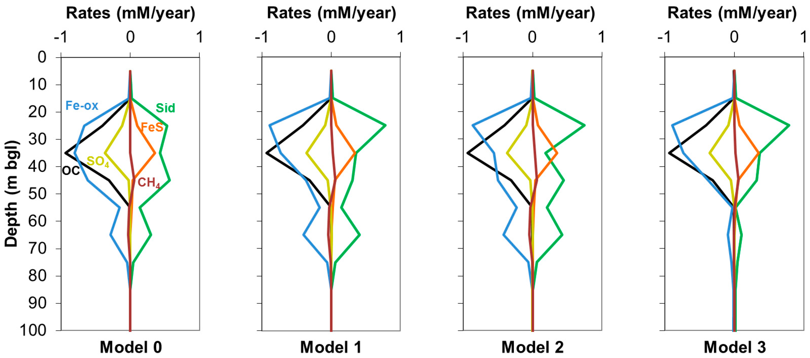
  • Model 1—this model considered a threshold energy for TEAPs (i.e., Fe-oxide reduction, sulfate reduction, and methanogenesis) on a unidirectional reaction using the “extended partial equilibrium” approach [29].
  • Model 2—this model implemented a bidirectional threshold energy for the Fe(III)/Fe(II) redox pair, which is the “extended partial equilibrium” approach with the “energy gap” for this reaction pair, in a similar manner to what Jakobsen [28] considered for the redox reaction pair methanogenesis/methane oxidation; sulfate reduction and methanogenesis were modeled using a unidirectional threshold energy.
  • Model 3—this model implemented a bidirectional threshold energy for the redox pair methanogenesis/methane oxidation; Fe-oxide reduction and sulfate reduction were modeled using a unidirectional threshold energy.
It has not yet been possible to make a working model combining a bidirectional threshold energy for more than one redox reaction pair at a time. All models simulated 1D reactive transport using PHREEQC [39] and the wateq4f database [40], slightly modified for Models 1–3, considering a downward flow through a vertical column composed of 12 cells of 10 m (Table 1). This thickness represents the first 120 m of depth comprising the first three aquifers (i.e., U, S, and C1) and aquitards. Within this domain, coherent hydrogeological properties and hydrodynamics enable a simplification of the system in a 1D model [11]. Model calibration was performed by trial and error adjusting the sensitive parameters in order to fit modeled concentrations to field data. Eight wells were used for the calibration process. These wells are located in a sub-portion of the study area that meets the assumptions for 1D modeling [11].

2.4. Model Settings and Calibration

2.4.1. Model 0

Model 0 refers to the model presented in the previous work by Rotiroti et al. [11]. This was based on the “partial equilibrium” approach [38] that involves the subdivision of the degradation of OM into two steps: (a) the hydrolyzation and fermentation of OM with the production of simpler compounds such as formic acid, acetic acid, H2, and CO2; and (b) the consumption of the fermentative products by TEAPs. The first step controls the overall rate, whereas TEAPs are assumed to approach equilibrium. This approach seems to fit the studied system since the main processes governing As concentrations occur close to a concomitant equilibrium, as highlighted in the conceptual model. In particular, the “partial equilibrium” approach was considered for simulating Fe-oxide reduction, sulfate reduction, and methanogenesis. The stoichiometry of these reactions is shown in Table 2.
A steady-state flow with a constant vertical downward flow was used. The vertical flow velocity was 3.12 m/year, and the diffusion coefficient was 0.3 × 10⁻⁹ m2/s with no dispersion [11]. The total simulation period of ~160 years allowed the biogeochemistry of the system to reach a quasi-steady-state [11].
The hydrogeochemical conceptual model was simulated through the following reaction network [11]:
  • Irreversible reactions: (a) oxidation of OM sourced by peat as (CH2O)106(NH3)4.5(H3PO4), producing inorganic C, NH4, and inorganic P; and (b) the reductive dissolution of Mn-oxide driven by adding Mn-oxide to the reduced system.
  • Equilibrium reactions: (a) the reductive dissolution of Fe-oxide with trace As(V); (b) the precipitation of calcite, dolomite, siderite, and rhodochrosite; and (c) the precipitation of FeS with trace As(III).
Model 0 calibration was done by adjusting: (a) the rate of OM degradation, (b) the SI of the Fe-oxide, (c) the SI of the FeS, and (d) the content of As in both Fe-oxide and FeS (see Rotiroti et al. [11] for details).

2.4.2. Model 1

This model extends Model 0 by implementing a threshold energy for unidirectional TEAP reactions. This matches the “extended partial equilibrium” approach, as defined by Jakobsen and Cold [29], since the energy needed for the bacteria to carry out the microbiologically mediated processes is included in the thermodynamic description of the system. This energy requirement needed for the microorganisms to mediate the reaction is implemented in the model by considering a threshold energy for the occurrence of the reaction. So, the reactions only proceed if the energy available to the bacteria mediating the processes exceeds a threshold. This threshold energy was implemented in the model by shifting the logK value of the reaction to lower or higher values, depending on the direction of the reaction. The difference between the logK and the shifted logK in terms of Gibbs energy is the threshold energy, that is, in other words, the energy required in the system to make the reaction microbiologically feasible. Along the lines of Hoehler [31], followed by subsequent works [28,29], who proposed that the H2 level may reflect the internal redox state of many different types of anaerobic microorganisms, regardless of the main electron donor used, TEAP reactions were rewritten in the PHREEQC database considering the H2 as the reductant instead of electrons. This also enables a comparison of results with previous works [28,29,31], as well as checking if the modeled H2 levels are reasonable compared to values typical for natural systems. The “extended partial equilibrium” approach was considered for Fe-oxide reduction, sulfate reduction, and methanogenesis. Their rewritten reactions using H2 are listed in Table 3.
Concerning Model 1 settings, the geometries, chemistry, geochemical boundary conditions, and calibrated parameters were the same as in Model 0. Changes were made only on the notation of TEAPs reactions, as explained above, and on the logK values of the reactions that were shifted to implement the threshold energy. Calibration of Model 1 was done by adjusting only the shifted logK value for Fe reduction, sulfate reduction, and methanogenesis.
The threshold energy was expressed in terms of kJ/mol of electrons and was calculated as the difference between the logK and the shifted logK, which was then converted using Van’t Hoff and Gibbs-Helmholtz equations, as described by Jakobsen and Cold [29]. The calculated threshold energy values were referred to the temperature of 15 °C used in the PHREEQC simulation and corresponding to values measured in the field.

2.4.3. Models 2 and 3

Models 2 and 3 extend Model 1 by implementing a bidirectional threshold energy for TEAP reactions, that are potentially reversible [41]. This also alleviates the problem associated with using the “extended partial equilibrium” approach with shifted logK values, as this implies that reactions may run in reverse with a loss of energy if conditions change. In Model 2, the bidirectional threshold energy is implemented for the redox reaction pair Fe(III) reduction/Fe(II) oxidation, since the reduction of Fe-oxide is an important process in the studied system, being the main mechanism responsible for As release [12,34]. In order to model this reversibility considering the threshold energy, ensuring that both the microbiologically mediated Fe(III) reduction and Fe(II) oxidation only occur when the amount of energy available exceeds the threshold energy needed for the given reaction, the simple use of shifting the logK value is not possible since this method can only work on a single direction. To overcome this limitation, a BASIC algorithm within the kinetic feature of PHREEQC was used, as done by Jakobsen [28] for methanogenesis/methane oxidation. The BASIC algorithm is used to find the amount of reaction necessary to reach the threshold energy on the basis of a calculation of the Gibbs energy for Fe(III) reduction or Fe(II) oxidation from the activities of reactants and products involved in the process. If the system is in a state where there is too little energy for any of the processes, no reaction occurs and the “energy gap” is created in which neither the reduction nor oxidation of Fe occurs [28]. For details on the BASIC algorithm see the Supplementary Materials that contain the full PHREEQC input file for Model 2 (Data File S1). The use of this algorithm needed some modifications in the wateq4f database since it requires the definition of distinct variables for the element Fe between oxidation state III (variable called “Feox”) and II (“Fered”). The modified database is available in the Supplementary Materials (Data File S2).
Basic settings of Model 2 were the same as in Model 0 and 1. Concerning the TEAPs, sulfate reduction and methanogenesis were the same as in Model 1 (i.e., their threshold energies were modeled using logK shifting). The change was only made for Fe, since Model 2 implements the “energy gap” for the reaction pair Fe(III) reduction/Fe(II) oxidation, as described above. The imposed threshold energy values for Fe(III) reduction, sulfate reduction, and methanogenesis were the same as in Model 1. Concerning Fe(II) oxidation, the same threshold energy as for Fe(III) reduction was used. The proper functioning of the BASIC script was checked by calculating the Gibbs free energy of reaction (the “dGrT_Fe” in Data File S1) and comparing it with the imposed threshold energy.
In Model 3, the bidirectional threshold energy is implemented for the redox reaction pair methanogenesis/methane oxidation, whereas Fe-oxide and sulfate reductions are modeled using a unidirectional threshold energy through logK shifting. The use of the bidirectional threshold energy for methanogenesis/methane oxidation became needful since the results (see below) showed that considerable methane oxidation occurred in the deeper part of the system. The threshold energy values imposed were the same as in Models 1 and 2; methane oxidation was modeled by imposing the same threshold value as for methanogenesis. The full PHREEQC input file for Model 3 and the related modified database are available in the Supplementary Materials (Data Files S3 and S4, respectively).

3. Results and Discussion

Figure 1 shows the comparison of measured and simulated concentrations by Model 0 with those simulated by the three newly developed models (Models 1, 2, and 3). Although H2 and CH4 were not measured in the field [12], they are represented in Figure 1 to check the validity of their concentrations in comparison with literature values. Figure 2 shows the modeled rates of main processes characterizing the system for Models 0, 1, 2, and 3. Table 3 reports the imposed threshold energy values that ensured the best model fits.
The results of Model 0 are described in detail in Rotiroti et al. [11]. However, in general, it can be stated that the good fit obtained suggests that the “partial equilibrium” approach, used for simulating the reaction network proposed in the conceptual model, can be a valid method for representing the hydrogeochemistry of the system.
Simulated concentration profiles of Model 1 are very similar to those of Model 0 (Figure 1). The sole significant variation in the concentration profiles is observed for H2, which has higher values with respect to Model 0. This is consistent with the implementation of a threshold energy for TEAPs. Indeed, the adoption of an energy requirement needed for the occurrence of TEAP reactions leads to a relative accumulation in the groundwater of H2 (which is a reactant in the imposed TEAP reactions) with respect to Model 0, where TEAPs are free to evolve without any energy requirements. Simulated H2 concentrations were generally within 1–10 nM that is a typical range of values observed in natural systems [28,29,42]. Simulated methane concentrations were below 0.4 mM, which are values comparable with those observed in other natural anoxic aquifers worldwide, such as the Red River floodplain in Vietnam [25,26] and the Asserbo [29] and Rømø [43] aquifers in Denmark.
The optimal threshold energies fitted for Model 1 were 3.76, 4.50, and 1.60 kJ/mol e for Fe-oxide reduction, sulfate reduction, and methanogenesis, respectively (Table 3). These results are consistent with literature values, such as 11.8 kJ/mol e for Fe-oxide reduction [29], 4.9 [29] and 2.4 [31] kJ/mol e for sulfate reduction, and 2.7 [29] and 1.3 [31] kJ/mol e for methanogenesis. That these threshold energy values are quite close and quite small indicates that the simpler “partial equilibrium” approach to modeling anaerobic redox processes is also viable.
A comparison of modeled reaction rates between Models 0 and 1 (Figure 2) shows that the rates are quite similar, with the exception of Fe-oxide reduction and siderite precipitation where, in Model 1, the peak of rates are moved upwards in the depth range 20–30 m bgl. Therefore, in Model 1, there is a sequence of rate peaks over depth for the different TEAPs that follows the canonical order of the ecological succession of TEAPs [44]. First the peak of Fe-oxide reduction between 20 and 30 m bgl, then for sulfate reduction between 30 and 40 m bgl, and finally the peak in methanogenesis between 40 and 50 m bgl. So, although these three processes still occur concomitantly, they occur with different rates over depth. Therefore, it appears that implementing a minimum energy requirement for the occurrence of TEAPs leads to a fit which complies closer to the generally observed succession of TEAPs. In general, it emerges from this modeling that the use of threshold energies has a higher influence on modeled rates rather than modeled concentrations (except for H2). Therefore, the availability of rate observations from in situ or batch experiments and H2 concentration measurements could help to constrain the model fit when threshold energies are implemented.
Simulated concentrations in Model 2 were very close to those in Model 1 (Figure 1), maintaining a good fit with measured concentrations. Moreover, reaction rates of Model 2 were also quite close to those of Model 1 (Figure 2). This agreement within results between Models 2 and 1 is related to the fact that no net reoxidation of Fe2+ to Fe3+ occurred in the system. Indeed, a closer analysis of results (i.e., same profile of modeled Fe3+ over depth for all models and no precipitation of newly formed Fe-oxide) confirms that in this simple 1D model there is no net reoxidation of Fe2+ to Fe3+. This explains why modeled concentrations and reaction rates are so similar in the two models, since similar results are expected if the net reoxidation of Fe2+ does not occur. The reason for this is that, in principle, modeling a bidirectional threshold energy when the reverse reaction is negligible is equivalent to modeling a unidirectional threshold energy. The fact that Models 1 and 2 gave the same results when there is no net reoxidation of Fe2+ confirms the robustness of both techniques used for modeling the threshold energy (i.e., the logK shifting and the BASIC algorithm calculating the amount of reaction necessary to reach the threshold energy).
The non-occurrence of the net reoxidation of Fe2+ in this case could be related to the use of a simple 1D model, allowing a stability of anoxic conditions that ensures the primary occurrence of Fe3+ reduction. However, in 2D or 3D simulations where reduced water may come into contact with more oxic waters downstream, it is very important to avoid the reoxidation of Fe2+. If this would occur using the logK shifting method as for Model 1, the oxidation would actually occur with a loss of energy, which would obviously be wrong.
As opposed to Fe-oxide and sulfate reductions, which showed a negligible occurrence of their reverse reactions (i.e., Fe2+ and sulfide reoxidation), simulated methane in Models 1 and 2 was subjected to formation in the shallower part of the system (down to 50 m bgl) with a rate of up to ~60 µM/year and oxidation in the deeper part (between 50 and 80 m bgl) with a rate of up to ~45 µM/year. The use of the logK shifting method for methanogenesis as done in Models 1 and 2 implied the simulation of the reverse methane oxidation with an erroneous loss of energy (as explained in Section 2.4.3). In order to overcome this limitation, Model 3 implemented a bidirectional threshold energy for the pair methanogenesis/methane oxidation.
Reaction rates simulated in Model 3 (Figure 2) were, in general, consistent with those of Models 1 and 2; a slight difference is seen in the deeper part of the system where the rates of Fe-oxide reduction and siderite precipitation decreased. This is related to the most notable change: the rate of methane oxidation, occurring in cells 6 (50–60 m bgl), 7 (60–70 m bgl), and 8 (70–80 m bgl), showed a decrease in Model 3 (0, 6, and 4 µM/year, respectively for these three cells) with respect to Model 1 (25, 44, and 7 µM/year, respectively) and Model 2 (33, 46, and 7 µM/year, respectively). This stems from the implementation of a threshold energy for methane oxidation in Model 3, preventing its occurrence with a loss of energy, as occurred in Models 1 and 2. This change in the modeling approach also had an effect on the simulated concentration of CH4. Indeed, Model 3 obtained a higher CH4 value in the deeper part of the system with respect to Models 1 and 2 (Figure 1) due to the lower rates of methane oxidation. This can also explain the lower H2 concentration simulated by Model 3, since hydrogen is a product of methane oxidation (Table 3), implying higher hydrogen levels in Models 1 and 2. Model 3 also showed a lower simulated pH. In all models, pH increases over depth due to the ongoing Fe-oxide reduction [45]; when methanogenesis is occurring concomitantly, this also controls the pH according to the following reaction shown in Equation (1):
16H+ + CH4 + 8Fe(OH)3 ↔ 8Fe2+ + CO2 + 22H2O.
In Model 3, the pH is lower likely because the lower methane oxidation implies a lower consumption of H+.

4. Conclusions

This work presented reactive transport modeling using a stepwise approach with increasing degrees of complexity for simulating the release and attenuation of As in groundwater by implementing the minimum Gibbs energy required by bacteria (i.e., threshold energy) to conduct TEAP reactions.
Although many aspects of this work remain theoretical (i.e., no measurements of CH4 and H2 concentrations, no rate observations, and no estimations of microbial biomass involved in the processes), some general points and indications for a wider applicability of this method can be drawn:
  • The “partial equilibrium” approach can be extended to comply more closely to the energy requirements of the microorganisms mediating TEAP processes with the aim of better understanding the hydro-bio-geochemistry of the aquifer system under analysis.
  • The use of a threshold energy, with the aim of incorporating the role of reaction mediation played by bacteria into reactive transport modeling, has some influence on the fitted rates of the modeled processes and on modeled H2 concentrations. So, implementing a threshold energy in reactive transport modeling could be useful when rate measurements and/or measured threshold values of H2 from in situ or batch experiments of microbially mediated processes are available. Imposing a threshold energy and using observations of rates and H2 concentrations would help to constrain the model fit.
  • The implementation of a threshold energy for only the reduction processes may lead to obviously faulty reverse reactions occurring with a loss of energy. This would occur in systems with a changing condition, e.g., anoxic water that subsequently seeped into oxic sediments, and implementing 2D or 3D models that involve more complex groundwater flow paths, facilitating a mixing of different redox conditions. However, our 1D modeling indicates that in simpler flow systems and under stable anoxic conditions, the problem of reverse oxidation reactions occurring with a loss of energy is negligible for some redox reaction pairs (e.g., Fe(III) reduction/Fe(II) oxidation), so the use of a unidirectional threshold energy simulated through the logK shifting method could be suitable in these cases.
  • By implementing a description of the redox process pairs that has the “energy gap”, the artefact of faulty reverse reactions occurring with a loss of energy can be avoided. The use of the bidirectional energy gap description is required in 1D modeling for those reaction pairs that alternate their preferential reaction direction, as occurred in our modeling for methanogenesis/methane oxidation, and is recommended for all the important TEAPs in 2D or 3D models involving more complex groundwater flow paths which can facilitate a mixing of anoxic and oxic conditions where, for instance, both methane and Fe2+ would be oxidized.
  • The main advantages and disadvantages of implementing a threshold energy in reactive transport modeling that emerge from this study are: (a) including threshold energies makes it possible to include H2 data when calibrating; (b) models implementing a bidirectional threshold energy take much longer to run and often show convergence problems; (c) unidirectional threshold energies cannot be used when reoxdation occurs within the model.
Future works involving the modeling of As release and attenuation in the Po Plain aquifers will be addressed, considering a 2D model, and thus, a bidirectional threshold energy for all the TEAPs considered, in particular for the reaction pairs Fe(III) reduction/Fe(II) oxidation, sulfate reduction/sulfide oxidation, and methanogenesis/methane oxidation. The use of micro-niches for the reaction pair methanogenesis/methane oxidation [28] will also improve the understanding of this system. Moreover, the role played by bacteria in mediating the reduction of As(V) to As(III) [46] will also be implemented using a threshold energy.

Supplementary Materials

The following are available online at www.mdpi.com/2073-4441/10/1/90/s1, Data File S1: PHREEQC input file for Model 2, Data File S2: Modified wateq4f database for running Model 2, Data File S3: PHREEQC input file for Model 3, and Data File S4: Modified wateq4f database for running Model 3.

Acknowledgments

Costs to publish in open access were covered by the University of Milano-Bicocca through the FAR fund No. 2014-ATE-0389 “Reconstruction and evolution of geo-environmental systems through the integration of field data, remote sensing, database and environmental modeling”.

Author Contributions

M.R. and R.J. conceived and designed the modeling; M.R. performed the modeling; R.J. revised the modeling; T.B. and L.F. contributed materials and analysis tools and supervised the work; M.R. and R.J. wrote the paper; T.B. and L.F. revised the paper.

Conflicts of Interest

The authors declare no conflict of interest.

References

  1. Ravenscroft, P.; Brammer, H.; Richards, K. Arsenic Pollution: A Global Synthesis; Wiley-Blackwell: Chichester, UK, 2009. [Google Scholar]
  2. Nickson, R.; McArthur, J.; Burgess, W.; Ahmed, K.M.; Ravenscroft, P.; Rahmann, M. Arsenic poisoning of Bangladesh groundwater. Nature 1998, 395, 338. [Google Scholar] [CrossRef] [PubMed]
  3. Burgess, W.G.; Pinto, L. Preliminary observations on the release of arsenic to groundwater in the presence of hydrocarbon contaminants in UK aquifers. Mineral. Mag. 2005, 69, 887–896. [Google Scholar] [CrossRef]
  4. McArthur, J.M.; Ravenscroft, P.; Safiulla, S.; Thirlwall, M.F. Arsenic in groundwater: Testing pollution mechanisms for sedimentary aquifers in Bangladesh. Water Resour. Res. 2001, 37, 109–117. [Google Scholar] [CrossRef]
  5. Ravenscroft, P.; McArthur, J.M.; Hoque, B.A. Geochemical and palaeohydrological controls on pollution of groundwater by arsenic. In Arsenic Exposure and Health Effects IV; Chappell, W.R., Abernathy, C.O., Calderon, R., Eds.; Elsevier Science: Oxford, UK, 2001; pp. 53–78. [Google Scholar]
  6. Lawson, M.; Polya, D.A.; Boyce, A.J.; Bryant, C.; Ballentine, C.J. Tracing organic matter composition and distribution and its role on arsenic release in shallow Cambodian groundwaters. Geochim. Cosmochim. Acta 2016, 178, 160–177. [Google Scholar] [CrossRef]
  7. McArthur, J.M.; Ravenscroft, P.; Sracek, O. Aquifer arsenic source. Nat. Geosci. 2011, 4, 655–656. [Google Scholar] [CrossRef]
  8. Neumann, R.B.; Ashfaque, K.N.; Badruzzaman, A.B.M.; Ali, M.A.; Shoemaker, J.K.; Harvey, C.F. Reply to ‘Aquifer arsenic source’. Nat. Geosci. 2011, 4, 656. [Google Scholar] [CrossRef]
  9. Carraro, A.; Fabbri, P.; Giaretta, A.; Peruzzo, L.; Tateo, F.; Tellini, F. Effects of redox conditions on the control of arsenic mobility in shallow alluvial aquifers on the Venetian Plain (Italy). Sci. Total Environ. 2015, 532, 581–594. [Google Scholar] [CrossRef] [PubMed]
  10. Dalla Libera, N.; Fabbri, P.; Mason, L.; Piccinini, L.; Pola, M. Geostatistics as a tool to improve the natural background level definition: An application in groundwater. Sci. Total Environ. 2017, 598, 330–340. [Google Scholar] [CrossRef] [PubMed]
  11. Rotiroti, M.; Jakobsen, R.; Fumagalli, L.; Bonomi, T. Arsenic release and attenuation in a multilayer aquifer in the Po Plain (northern Italy): Reactive transport modeling. Appl. Geochem. 2015, 63, 599–609. [Google Scholar] [CrossRef]
  12. Rotiroti, M.; Sacchi, E.; Fumagalli, L.; Bonomi, T. Origin of arsenic in groundwater from the multi-layer aquifer in Cremona (northern Italy). Environ. Sci. Technol. 2014, 48, 5395–5403. [Google Scholar] [CrossRef] [PubMed]
  13. Zavatti, A.; Attramini, D.; Bonazzi, A.; Boraldi, V.; Malagò, R.; Martinelli, G.; Naldi, S.; Patrizi, G.; Pezzera, G.; Vandini, W.; et al. La presenza di arsenico nelle acque sotterranee della Pianura Padana: Evidenze ambientali e ipotesi geochimiche “Occurrence of groundwater arsenic in the Po Plain: Environmental evidences and geochemical hypothesis”. Quad. Geol. Appl. 1995, S2, 2.301–2.326. [Google Scholar]
  14. Banfield, J.F.; Nealson, K.H. Geomicrobiology: Interactions between Microbes and Minerals; Reviews in Mineralogy and Geochemistry; Mineralogical Society of America: Washington, DC, USA, 1997; Volume 35. [Google Scholar]
  15. Chapelle, H.F. The significance of microbial processes in hydrogeology and geochemistry. Hydrogeol. J. 2000, 8, 41–46. [Google Scholar] [CrossRef]
  16. Islam, F.S.; Gault, A.G.; Boothman, C.; Polya, D.A.; Charnock, J.M.; Chatterjee, D.; Lloyd, J.R. Role of metal-reducing bacteria in arsenic release from Bengal delta sediments. Nature 2004, 430, 68–71. [Google Scholar] [CrossRef] [PubMed]
  17. Guo, H.; Zhou, Y.; Jia, Y.; Tang, X.; Li, X.; Shen, M.; Lu, H.; Han, S.; Wei, C.; Norra, S.; et al. Sulfur cycling-related biogeochemical processes of arsenic mobilization in the western Hetao Basin, China: Evidence from multiple isotope approaches. Environ. Sci. Technol. 2016, 50, 12650–12659. [Google Scholar] [CrossRef] [PubMed]
  18. Cavalca, L.; Corsini, A.; Zaccheo, P.; Andreoni, V.; Muyzer, G. Microbial transformations of arsenic: Perspectives for biological removal of arsenic from water. Future Microbiol. 2013, 8, 753–768. [Google Scholar] [CrossRef] [PubMed]
  19. Corsini, A.; Zaccheo, P.; Muyzer, G.; Andreoni, V.; Cavalca, L. Arsenic transforming abilities of groundwater bacteria and the combined use of Aliihoeflea sp. strain 2WW and goethite in metalloid removal. J. Hazard. Mater. 2014, 269, 89–97. [Google Scholar] [CrossRef] [PubMed]
  20. Bethke, C.M.; Sanford, R.A.; Kirk, M.F.; Jin, Q.; Flynn, T.M. The thermodynamic ladder in geomicrobiology. Am. J. Sci. 2011, 311, 183–210. [Google Scholar] [CrossRef]
  21. Jin, Q.; Bethke, C.M. A new rate law describing microbial respiration. Appl. Environ. Microbiol. 2003, 69, 2340–2348. [Google Scholar] [CrossRef] [PubMed]
  22. Jin, Q.; Bethke, C.M. The thermodynamics and kinetics of microbial metabolism. Am. J. Sci. 2007, 307, 643–677. [Google Scholar] [CrossRef]
  23. Colombani, N.; Mastrocicco, M.; Prommer, H.; Sbarbati, C.; Petitta, M. Fate of arsenic, phosphate and ammonium plumes in a coastal aquifer affected by saltwater intrusion. J. Contam. Hydrol. 2015, 179, 116–131. [Google Scholar] [CrossRef] [PubMed]
  24. Kocar, B.D.; Benner, S.G.; Fendorf, S. Deciphering and predicting spatial and temporal concentrations of arsenic within the Mekong Delta aquifer. Environ. Chem. 2014, 11, 579–594. [Google Scholar] [CrossRef]
  25. Postma, D.; Larsen, F.; Minh Hue, N.T.; Duc, M.T.; Viet, P.H.; Nhan, P.Q.; Jessen, S. Arsenic in groundwater of the Red River floodplain, Vietnam: Controlling geochemical processes and reactive transport modeling. Geochim. Cosmochim. Acta 2007, 71, 5054–5071. [Google Scholar] [CrossRef]
  26. Postma, D.; Pham, T.K.T.; Sø, H.U.; Hoang, V.H.; Vi, M.L.; Nguyen, T.T.; Larsen, F.; Pham, H.V.; Jakobsen, R. A model for the evolution in water chemistry of an arsenic contaminated aquifer over the last 6000 years, Red River floodplain, Vietnam. Geochim. Cosmochim. Acta 2016, 195, 277–292. [Google Scholar] [CrossRef] [PubMed]
  27. Rawson, J.; Siade, A.; Sun, J.; Neidhardt, H.; Berg, M.; Prommer, H. Quantifying reactive transport processes governing arsenic mobility after injection of reactive organic carbon into a Bengal Delta aquifer. Environ. Sci. Technol. 2017, 51, 8471–8480. [Google Scholar] [CrossRef] [PubMed]
  28. Jakobsen, R. Redox microniches in groundwater: A model study on the geometric and kinetic conditions required for concomitant Fe oxide reduction, sulfate reduction, and methanogenesis. Water Resour. Res. 2007, 43, W12S12. [Google Scholar] [CrossRef]
  29. Jakobsen, R.; Cold, L. Geochemistry at the sulfate reduction–methanogenesis transition zone in an anoxic aquifer—A partial equilibrium interpretation using 2D reactive transport modeling. Geochim. Cosmochim. Acta 2007, 71, 1949–1966. [Google Scholar] [CrossRef]
  30. Jin, Q.; Bethke, C.M. Cellular energy conservation and the rate of microbial sulfate reduction. Geology 2009, 37, 1027–1030. [Google Scholar] [CrossRef]
  31. Hoehler, T.M.; Alperin, M.J.; Albert, D.B.; Martens, C.S. Apparent minimum free energy requirements for methanogenic Archaea and sulfate-reducing bacteria in an anoxic marine sediment. FEMS Microbiol. Ecol. 2001, 38, 33–41. [Google Scholar] [CrossRef]
  32. West, J.M.; McKinley, I.G.; Palumbo-Roe, B.; Rochelle, C.A. Potential impact of CO2 storage on subsurface microbial ecosystems and implications for groundwater quality. Energy Procedia 2011, 4, 3163–3170. [Google Scholar] [CrossRef]
  33. Rotiroti, M.; Di Mauro, B.; Fumagalli, L.; Bonomi, T. COMPSEC, a new tool to derive natural background levels by the component separation approach: Application in two different hydrogeological contexts in northern Italy. J. Geochem. Explor. 2015, 158, 44–54. [Google Scholar] [CrossRef]
  34. Rotiroti, M.; McArthur, J.; Fumagalli, L.; Stefania, G.A.; Sacchi, E.; Bonomi, T. Pollutant sources in an arsenic-affected multilayer aquifer in the Po Plain of Italy: Implications for drinking-water supply. Sci. Total Environ. 2017, 578, 502–512. [Google Scholar] [CrossRef] [PubMed]
  35. McArthur, J.M.; Banerjee, D.M.; Hudson-Edwards, K.A.; Mishra, R.; Purohit, R.; Ravenscroft, P.; Cronin, A.; Howarth, R.J.; Chatterjee, A.; Talukder, T.; et al. Natural organic matter in sedimentary basins and its relation to arsenic in anoxic ground water: The example of West Bengal and its worldwide implications. Appl. Geochem. 2004, 19, 1255–1293. [Google Scholar] [CrossRef]
  36. Fendorf, S.; Michael, H.A.; van Geen, A. Spatial and temporal variations of groundwater arsenic in South and Southeast Asia. Science 2010, 328, 1123–1127. [Google Scholar] [CrossRef] [PubMed]
  37. Lowers, H.A.; Breit, G.N.; Foster, A.L.; Whitney, J.; Yount, J.; Uddin, M.N.; Muneem, A.A. Arsenic incorporation into authigenic pyrite, Bengal Basin sediment, Bangladesh. Geochim. Cosmochim. Acta 2007, 71, 2699–2717. [Google Scholar] [CrossRef]
  38. Postma, D.; Jakobsen, R. Redox zonation: Equilibrium constraints on the Fe(III)/SO4-reduction interface. Geochim. Cosmochim. Acta 1996, 60, 3169–3175. [Google Scholar] [CrossRef]
  39. Parkhurst, D.L.; Appelo, C.A.J. Description of input and examples for PHREEQC version 3: A computer program for speciation, batch-reaction, one-dimensional transport, and inverse geochemical calculations. In U.S. Geological Survey Techniques and Methods, Book 6, Modeling Techniques; USGS: Reston, VA, USA, 2013; Chapter 43. [Google Scholar]
  40. Ball, J.W.; Nordstrom, D.K. Wateq4f—User’s Manual with Revised Thermodynamic Data Base and Test Cases for Calculating Speciation of Major, Trace and Redox Elements in Natural Waters; USGS Open-File Report 90-129; USGS: Reston, VA, USA, 1991.
  41. Christensen, T.H.; Bjerg, P.L.; Banwart, S.A.; Jakobsen, R.; Heron, G.; Albrechtsen, H.-J. Characterization of redox conditions in groundwater contaminant plumes. J. Contam. Hydrol. 2000, 45, 165–241. [Google Scholar] [CrossRef]
  42. Chapelle, F.H.; McMahon, P.B.; Dubrovsky, N.M.; Fujii, R.F.; Oaksford, E.T.; Vroblesky, D.A. Deducing the distribution of terminal electron-accepting processes in hydrologically diverse groundwater systems. Water Resour. Res. 1995, 31, 359–371. [Google Scholar] [CrossRef]
  43. Jakobsen, R.; Postma, D. In situ rates of sulfate reduction in an aquifer (Rømø, Denmark) and implications for the reactivity of organic matter. Geology 1994, 22, 1101–1106. [Google Scholar] [CrossRef]
  44. McMahon, P.B.; Chapelle, F.H. Redox processes and water quality of selected principal aquifer systems. Ground Water 2008, 46, 259–271. [Google Scholar] [CrossRef] [PubMed]
  45. Howell, J.R.; Donahoe, R.J.; Roden, E.E.; Ferris, F.G. Effects of microbial iron oxide reduction on pH and alkalinity in anaerobic bicarbonate-buffered media: Implications for metal mobility. Mineral. Mag. 1998, 62A, 657–658. [Google Scholar] [CrossRef]
  46. Osborne, T.H.; McArthur, J.M.; Sikdar, P.K.; Santini, J.M. Isolation of an arsenate-respiring bacterium from a redox front in an arsenic-polluted aquifer in West Bengal, Bengal basin. Environ. Sci. Technol. 2015, 49, 4193–4199. [Google Scholar] [CrossRef] [PubMed]
Figure 1. Measured vs. modeled molar concentrations of selected species over depth; symbol length corresponds to well screen interval; U, S, and C1 refer to unconfined, semi-confined, and confined 1 aquifer units, respectively; M0, M1, M2, and M3 refer to the four implemented models.
Water 10 00090 g001
Figure 2. Modeled rates of selected processes over depth; negative rates indicate consumption, positive formation; Fe-ox: Fe-oxide reduction; OC: organic carbon consumption; SO4: sulfate reduction; Sid: siderite precipitation; FeS: iron sulfide precipitation; CH4: methane formation/oxidation.
Water 10 00090 g002
Table 1. Model geometry and corresponding hydrogeological units.
CellDepth (m bgl)Hydrogeological Unit
10–10Aquifer U
210–20Aquifer U
320–30Aquitard U/S
430–40Aquifer S
540–50Aquifer S
650–60Aquifer S
760–70Aquitard S/C1
870–80Aquitard S/C1
980–90Aquifer C1
1090–100Aquifer C1
11100–110Aquifer C1
12110–120Aquitard C1/C2
Table 2. Stoichiometry of TEAP reactions implemented in Model 0.
NameReactionlogK
Fe-oxide reductionFe3+ + e ↔ Fe2+13.02
Sulfate reductionSO42− + 10H+ + 8e ↔ H2S + 4H2O40.64
MethanogenesisCO32− + 10H+ + 8e ↔ CH4 + 3H2O41.07
Table 3. Stoichiometry of TEAP reactions implemented in Models 1, 2, and 3 and optimal threshold energy values obtained.
NameReactionlogKShifted logK 1Threshold Energy (kJ/mol e)
Fe-oxide reductionFe3+ + 0.5H2 ↔ Fe2+ + H+14.5513.873.76 2
Sulfate reductionSO42− + 2H+ + 4H2 ↔ H2S + 4H2O52.9646.444.50
MethanogenesisHCO3 + H+ + 4H2 ↔ CH4 + 3H2O40.1837.861.60 3
1 Not considered for Fe-oxide reduction in Model 2 and for methanogenesis in Model 3; 2 used for both reaction directions in Model 2; 3 used for both reaction directions in Model 3.

