Characteristics of Atmospheric Boundary Layer Structure during PM2.5 and Ozone Pollution Events in Wuhan, China

1
Institute of Atmospheric Physics and Atmospheric Environment, School of Environmental Studies, China University of Geosciences, Wuhan 430074, China
2
Solomon Mahlangu College of Science and Education, Department of Geography and Environmental Studies, Sokoine University of Agriculture, Morogoro P.O. Box 3038, Tanzania
*
Author to whom correspondence should be addressed.
Atmosphere 2018, 9(9), 359; https://doi.org/10.3390/atmos9090359
Submission received: 17 July 2018
/
Revised: 30 August 2018
/
Accepted: 7 September 2018
/
Published: 18 September 2018
(This article belongs to the Special Issue Air Quality in China: Past, Present and Future)
Abstract
:In this study, we investigated six air pollutants from 21 monitoring stations scattered throughout Wuhan city by analyzing meteorological variables in the atmospheric boundary layer (ABL) and air mass backward trajectories from HYSPLIT during the pollution events. Together with this, ground meteorological variables were also used throughout the investigation period: 1 December 2015 to 30 November 2016. Analysis results during this period show that the city was polluted in winter by PM2.5 (particulate matter with aerodynamics of less than 2.5 microns) and in summer by ozone (O3). The most polluted day during the investigation period was 25 December 2015 with an air quality index (AQI) of 330 which indicates ‘severe pollution’, while the cleanest day was 26 August 2016 with an AQI of 27 indicating ‘excellent’ air quality. The average concentration of PM2.5 (O3) on the most polluted day was 265.04 (135.82) µg/m3 and 9.10 (86.40) µg/m3 on the cleanest day. Moreover, the percentage of days which exceeded the daily average limit of NO2, PM10, PM2.5, and O3 for the whole year was 2.46%, 14.48%, 23.50%, and 39.07%, respectively, while SO2 and CO were found to be below the set daily limit. The analysis of ABL during PM2.5 pollution events showed the existence of a strong inversion layer, low relative humidity, and calm wind. These observed conditions are not favorable for horizontal and vertical dispersion of air pollutants and therefore result in pollutant accumulation. Likewise, ozone pollution events were accompanied by extended sunshine hours, high temperature, a calm wind, a strongly suspended inversion layer, and zero recorded rainfall. These general characteristics are favorable for photochemical production of ozone and accumulation of pollutants. Apart from the conditions of ABL, the results from backward trajectories suggest trans-boundary movement of air masses to be one of the important factors which determines the air quality of Wuhan.
1. Introduction
In recent years, air pollution has been an area of concern of the public, governments, as well as academia. This is partly due to the rising awareness of the negative health consequences associated with air pollution, particularly in developing countries. Estimates from a report by the World Health Organization (WHO) suggest air pollution to be responsible for one in every nine deaths annually, while outdoor pollution alone kills around 3 million people each year. The report further reveals that only one in every ten persons resides in a city which complies with WHO air quality guidelines (AQG) [1]. China as one of the developing countries with the fastest economic growth is facing air pollution problems in most of its cities due to rapid urbanization and industrialization [2,3,4,5]. Currently, most of its cities are reported to be polluted mainly by PM2.5 (particulate matter with aerodynamics of less than 2.5 microns) in winter and by ozone (O3) in summer. As one of the mitigation measures to air pollution problems, the Chinese Ministry of Environmental Protection (CMEP) enacted National Ambient Air Quality Standard (NAAQS) in 2012 to regulate the emission of six principle pollutants (NO2, SO2, CO, O3, PM2.5, and PM10) to the atmosphere. The set limits for the daily average concentration of PM2.5 and 8 hours average concentration of ozone are 75 µg/m3 and 160 µg/m3, respectively, while the annual average limit concentration of PM2.5 is 35 µg/m3 [6]. These standards are far above the set AQG by WHO of a daily average of 25 µg/m3 for PM2.5 and 100 µg/m3 for 8 h average concentration of ozone, even though WHO acknowledges this heterogeneity [7]. It is worth noting that, these WHO AQGs were developed based on the extensive body of scientific evidence relating to air pollution and its health consequences.
Wuhan, (29°58′–31°22′ N and 113°41′–115°05′ E) is the largest city in central China and the capital city of Hubei province; the hub of transportation and the major link of the West and East. So far, the city has been reported to be polluted by a number of studies [8,9,10,11,12,13,14,15,16,17,18]. While literature on PM2.5 pollution in Wuhan is still limited compared to other major cities in China, it is apparently sufficient compared to the literature on ozone pollution which is the dominant pollutant during summer. A summary of some of the available literature on PM2.5 pollution is as follows. Lyu et al. [11] reveal that the quality of air in Wuhan is polluted because PM10 and PM2.5 frequently exceeded NAAQS as a result of intensive biomass burning. During the investigation period, they found the average concentration of PM2.5 to be 81 µg/m3 in summer and 85 µg/m3 in autumn. A sampling campaign by Acciai et al. [15] in spring found an average concentration of PM2.5 of 95 µg/m3 and by using the Positive Matrix Factorization (PMF) method, biomass burning was identified as the largest contributor (62%) of PM2.5 in Wuhan. Other identified sources were metallurgical and steel industries (14%), crustal dust (13%), and dust and vehicle emission (10%). Wang et al. [18] found the annual average concentration of PM2.5, PM10, and NO2 exceeded NAAQS by 256%, 192%, and 137%, respectively. For the whole year, monthly average concentration of PM2.5 was the highest in December and lowest in July as a result of precipitation. For the period of three years (2013‒2015), Xu et al. [17] found the concentration of PM2.5 and PM10 were above the daily acceptable limit by 40% and 27%, respectively. The average ratio of PM2.5/PM10 during these three years was 0.62 and the average ratio in winter was higher by 20% compared to the average ratio in summer. The authors also found gradual increase of the PM2.5/PM10 ratio at night time and they related this increase to stable atmospheric conditions which constrained vertical airflow. Mbululo et al. [14] reported the percentage of days in which the ratio of PM2.5 in PM10 was more than half, to be 83%, which indicates that the greater portion of pollutants in the city were composed of smaller particles. Moreover, the authors found higher concentration of elementary carbon (EC) prior to the PM2.5 episodes (three or more consecutive days of PM2.5 ≥ 75 µg/m3) and suggested biomass burning to be one of the reasons for the occurrence of the episodes.
With regard to ozone pollution, study by Gong et al. [16] using 2014‒2016 ozone data, ranked Wuhan as the fourth polluted city in China following Beijing, Chengdu, and Hangzhou after having 126 non-attainment days of ozone limit set by NAAQS. Three factors; Day of the year (DOY), daily average relative humidity at 1000 mb, and daily maximum temperature at 2 m height were identified as the leading factors for ozone pollution in Wuhan. Study by Qian et al. [12] on ambient air pollution and preterm birth in Wuhan observed a consistent but small association between PM2.5, PM10, CO, and O3 and preterm birth during the investigation period. The authors found that, for every 5 µg/m3 and 10 µg/m3 increase in PM2.5 and O3, there was an increase in the risk of preterm birth by 3% and 5%, respectively, when they considered exposure throughout the entire pregnancy. Likewise, the study by Zhang et al. [8] on maternal exposure to air pollutants suggests that the exposure to increased level of ozone in the first trimester of pregnancy may contribute to the risk of congenital heart defect (CHF). For the first time Lyu et al. [13] studied the characteristics and sources of volatile organic compounds (VOC) and their effect on ozone formation. The authors found liquefied petroleum gas and solvent in coating/painting to be the major contributor of ozone formation. A follow-up study to this went far to unveil the contribution of agricultural burning to ozone formation (18%) [19]. The authors suggest VOC control and a ban on agricultural biomass burning to be considered as a means of improving air quality in Wuhan.
Elsewhere, significant research work has been done concerning ozone pollution, more specifically on its sources [20,21], formation [2,3,22,23], measurement [24], adverse effect to human health [5,25,26], and effect on food crops [4,27,28,29]. Regarding the influence of meteorological variables to PM2.5 and ozone pollution, most of the available literature has concentrated on the ground meteorological variable and put aside the atmospheric boundary layer (ABL) which is the main determinant of air quality. This is partly because the surface variables are regularly well monitored but the vertical profiles of these variables are usually not monitored (except for weather radiosondes). For instance, the study by Shan et al. [30] found that high ozone days were mainly accompanied by sufficient sunshine duration, high temperature, and little rainfall. Equally, ozone episodes were also found to be associated with low wind speed and trans-boundary movement of air pollutant from highly polluted areas. Although other studies observed ABL, they did not analyze its evolution with respect to air quality. For instance, Tang et al. [31] suggest photochemical reactions to be the main reason for ozone dominance in the ABL because of the circulation between the lower and upper ABL, even though vertical diffusion is the main source of ozone near the ground. Based on the literature which we came across, it is clear that most of the authors have not given enough attention to the dynamics of the ABL, which is the major determinant of air quality [32,33]. Recently, Li et al. [34], studied the relationship of air pollutants and meteorological parameters by using instruments which are fixed at different heights on a 100 m tower. This altitude is not high enough to describe the dynamics of the ABL. Moreover, studies by Tang et al. [31] and Wang et al. [27] call for more detailed vertical studies on meteorological variables to fully understand the processes of the ABL because most previous studies were based on ground observation. Taking Wuhan city as an example, this study therefore sought to elucidate the dynamics of the atmospheric boundary layer (ABL) structure during pollution events. To attain this goal, ground observation data from meteorological stations, high altitude sounding data, air quality data together with the air mass back trajectories were used in this study.
2. Methodology
2.1. Data and Sampling Sites
This study used six monitored air pollutants (PM2.5, PM10, SO2, NO2, CO, and O3) from 21 stations which are distributed all over Wuhan. Within these stations, there are nine stations which are administered by the CMEP and are used to determine the AQI of the city, while the remaining 12 stations are administered by the local government authority (LGA). Details on how AQI is calculated have been elaborated clearly with the China National Environmental Protection Standard [35]. Together with this, daily L-band radar data at 0700 LST with a vertical resolution of 10 m was also used to describe the vertical profile of different meteorological variables (temperature, humidity, wind speed, and wind direction) up to 3000 m. The air quality data were obtained from Wuhan Environmental Protection Agency (WHEPA), while the L-band sounding data was obtained from the Wuhan Meteorological Bureau (WMB). The investigated period was from 1 December 2015 to 30 November 2016. Daily averaged data for PM2.5, O3, and AQI were used to plot the line graphs from which one could define highly polluted and clean days; L-band sounding data were used to plot the vertical profile of the meteorological elements.
2.2. Back-Trajectory Analysis
Airborne PM can be transported from one place to another by the movement air parcel. So, the air mass residence time over a specific source area is linearly related to that area’s contribution to the receptor site [36]. The 72 hour air mass back trajectories approaching Wuhan at 100 m, 300 m, and 600 m were used to calculate and analyze airflow and diffusion by using Hybrid Single-Particle Lagrangian Integrated Trajectory (HYSPLIT) developed by National Oceanic and Atmospheric Administration (NOAA) Air Resources Laboratory’s (ARL) of the United States. The software tool has a relatively complete transport, diffusion, and sedimentation model for handling a variety of meteorological element input fields, multiple physical processes, and different types of pollutant emission sources [37,38]. Meteorological data input was from NCEP (National Centers for Environmental Prediction) fields obtained from NOAA which are available at every 3 h with 1° × 1° spatial resolution.
2.3. Potential Source Contribution Function (PSCF)
A PSCF method was also used in this study to determine the major contributing areas of PM2.5 and O3 in Wuhan. The basis of PSCF is that if a receptor site is located at a particular latitude and longitude, an air parcel back trajectory passing through that location indicates that the material from other sources can be transported through the trajectory to the receptor site [39,40,41]. It is defined by the following Equation (1).
where, is the number of times that the trajectories passed through the cell (i,j) and is the number of times that the pollutant concentrations were higher at the receptor site than the set criterion. In this study, the set criteria for PM2.5 and O3 of 75 µg/m3 and 160 µg/m3, respectively were utilized in the PSCF calculation to identify the potential source areas (PSA) at distances which are more likely to have larger impact than the local sources. To reduce uncertainties resulting from the effect of simulation results of the grids with values of that are too small, an empirical weighting coefficient, (Equation (2)) was multiplied to the PSCF [40,41]. For the case of this study, is the average value () >0) of the number of all trajectory terminal points in grids:
2.4. Concentration Weighted Trajectory (CWT)
A CWT model was also used to produce the geographical overview of emission sources areas which enriched Wuhan with airborne PM. The CWT equation (3) yields a weighted concentration for each grid cell (i,j), based on the average daily air pollutant levels measured at the sampling site, corresponding to the trajectories overlying across this grid cell (i,j):
where, is the average weighted concentration in a grid cell (i,j), k is the index of the trajectory, v is the total number of the trajectories, Ck is the concentration observed on arrival of trajectory k, and is the time spent in the grid cell (i,j) by trajectory k [36,39,40]. This CWT algorithm was applied independently of PM2.5 and O3 in order to distinguish the origin of the air masses influence in Wuhan. The results of CWT were also multiplied with the same weight function (Equation (2)) in order to enhance the statistical stability.
3. Results and Discussion
3.1. Overview of Air Pollution in Wuhan
Analysis of the six monitored air pollutants (PM2.5, PM10, SO2, NO2, CO, and O3) which are used to calculate AQI in Wuhan show that the pollutants are above the NAAQS at different levels, except CO and SO2 which were within the set daily limit. The highest AQI recorded was 330 on 25 December 2015 and the lowest AQI was 27 on 26 August 2016, which indicate ‘severe pollution’ and ‘excellent’ air condition, respectively. The average concentration of PM2.5 (O3) during the highest AQI was 265 (135) µg/m3 and 9 (86) µg/m3 during the lowest AQI. According to the Chinese air grading standard [35] which is summarized in Table 1, for the whole year, ‘excellent’ days were 13%, ‘good’ days were 51%, ‘slightly polluted’ days were 24%, ‘moderate polluted’ days were 7%, ‘heavy polluted’ days were 3%, and ‘severe polluted’ days were 1%. The annual average levels of PM2.5 and PM10 from nine (9) air quality monitoring stations administered by CMEP were 59 µg/m3 and 94 µg/m3 which are far above the NAAQS of 35 µg/m3 and 70 µg/m3, respectively. In the case of annual average concentration of NO2, it was 46 mg/m3 while its acceptable limit is 40 mg/m3. Moreover, the percentage of days which exceeded the daily average limit for the whole year was 2%, of NO2, 14%, of PM10, 23% of PM2.5, and 39%, for O3, while SO2 and CO were far below the daily set limit of 150 µg/m3 and 4 mg/m3, respectively. One of the reasons as to why SO2 is within the set standard is because of the government initiatives taken in around the year 2005, which demanded the introduction of flue-gas desulfurization (FGD) in all power plants [42]. Moreover, PM2.5, PM10, and NO2 pollution were seen to be more dominant during winter, while O3 pollution was more dominant in summer and very low in winter. Looking at the annual average of 12 stations which are administered by the LGA, the PM2.5 has a concentration of 56 µg/m3 and PM10 has 89 µg/m3, which are also above the set standard. Furthermore, the correlation coefficient of the daily PM2.5 data from nine stations ranged from 0.92 to 0.99 which suggests the pollutants sources were the same. Monthly average of 9 (12) stations data show that, the top three months with high concentration of PM2.5 were December (January) with average concentration of 108 (100) µg/m3, January (December) with average concentration of 107 (91) µg/m3, and March (March) with 85 (82) µg/m3. The three months with the lowest PM2.5 concentration were July (July), June (June), and August (August), with average monthly concentrations of 25 (26) µg/m3, 32 (33) µg/m3, and 34 (36) µg/m3, respectively.
The three months with the highest concentration of ozone within 9 (12) stations were September (September) with average concentration of 186 (194) µg/m3, August (August) with 178 (180) µg/m3, and July (May) with 158 (161) µg/m3. It is worth highlighting at this juncture that, even though September is found to have high O3, it is not regarded as a summer month but rather an autumn month. The months with the lowest O3 concentration were December (January) with 58 (69) µg/m3, January (December) with 61 (77) µg/m3, and November (November) with 69 (81) µg/m3. During these summer months, the highest AQI was 138, which indicates that the air is ‘slightly polluted’ and the concentration of ozone was 210 µg/m3 on 17 June 2016. Moreover, the correlation coefficient between the nine stations data for O3 was between 0.79 and 0.96 suggesting the pollutant sources come from the same source. The small difference in concentration of PM2.5 and O3 recorded by stations administered by the CMEP and LGA is because they are located in different areas and experience contributions from different local emissions.
3.2. Analysis of PM2.5 and O3 Pollution during Winter and Summer
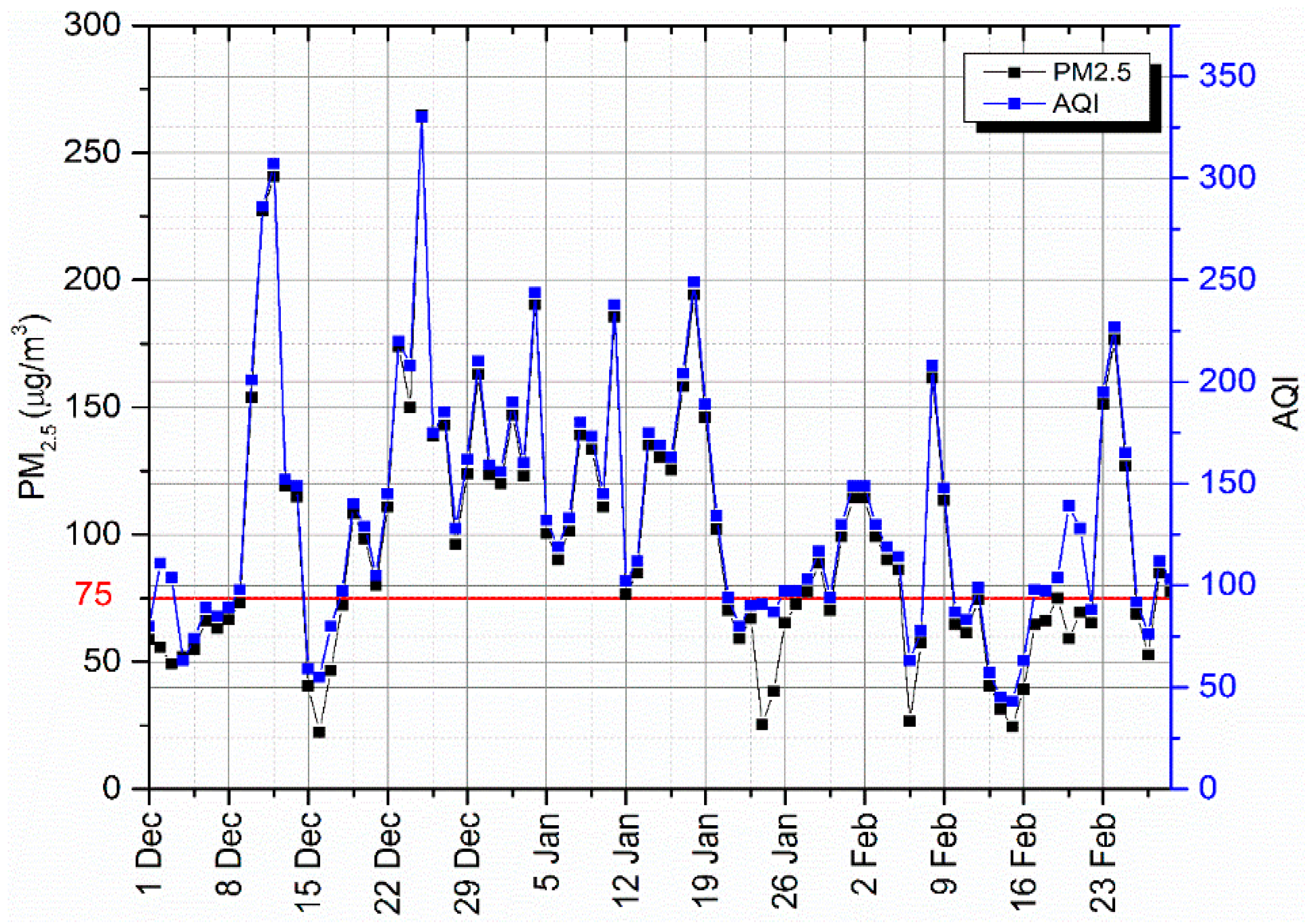
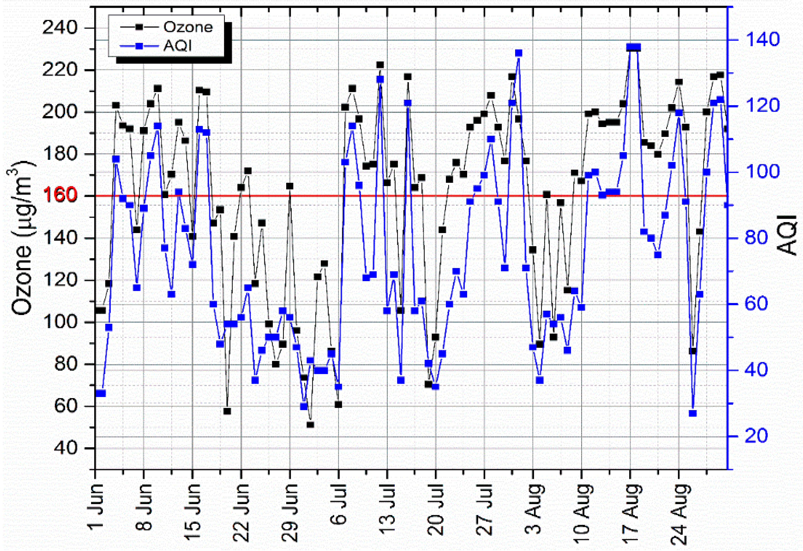
The variation of PM2.5 concentration and AQI from 1 December 2015 to 29 February 2016 are represented in Figure 1, where the daily concentration of PM2.5 is observed to exceed the set limit by 58%, while during the same period, PM10 was above the limit by 33%. During this three month period, PM2.5 was the primary pollutant by 78%, PM10 by 14%, and the remaining 8% was for NO2. A different scenario was observed during summer, as no single day in this period of three months exceeded the set limit and a small concentration of PM2.5 of 7 µg/m3 was recorded on 4 July 2016. Concerning ozone concentration, this was above the 8 hours average limit of 160 µg/m3 for 66% during June, July, and August (J-J-A) (Figure 2). Primary pollutants during this period of time were O3 by 88%, followed by PM10 with 10% and NO2 with 3%. These results suggest that PM2.5 pollution is a serious issue during the winter season and O3 pollution is dominant during summer. Therefore, there is a need for special initiatives to tackle these pollutants as they have been associated with negative impacts on human being as well as the environment. The order of pollution suggests that the stations which are near the city center (e.g., Hankou Jiangtao), where there is high traffic and dense population were more polluted, and the least polluted stations were those found at the outskirts of the city (e.g., Donghu Gaoxin) where there is less population. Corroborated results of this were reported by Song et al. [10] and Xu et al. [17]. To gain more insight, the pollution process and the dynamics of the ABL structure are presented in detail in the subsection below.
3.3. Analysis of PM2.5 Pollution Process
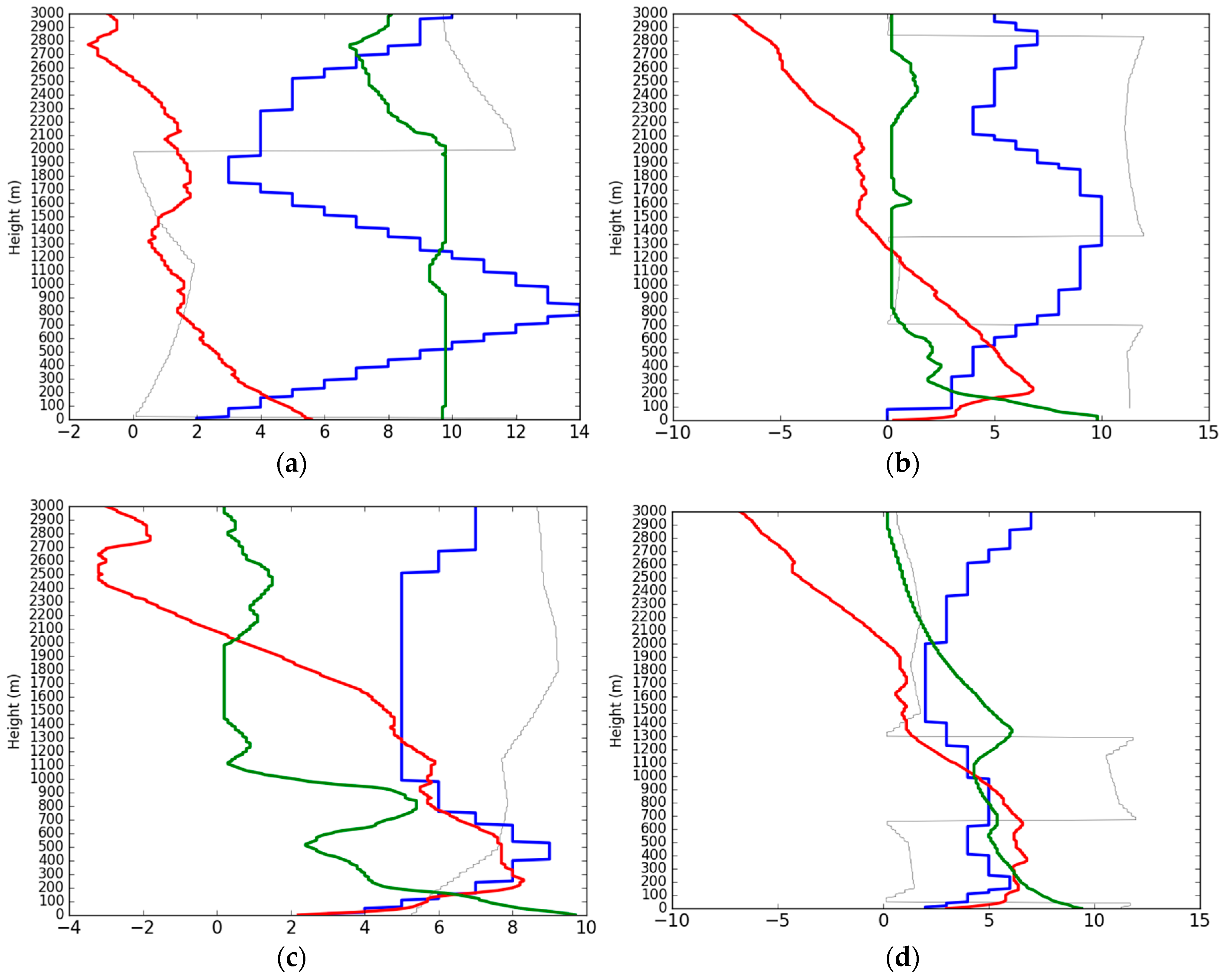
A clear PM2.5 pollution process can be seen from 3–28 December 2015 in Figure 1 where there was a continuous accumulation of PM2.5 concentration for 10 days and weakening for 4 days before it reached its minimum concentration on 16 December 2015. Thereafter, on 17 December 2015, pollutants began to accumulate again for another 10 days and weakened for 3 days before they reached their minimum level on 28 December 2015 (Figure 1). ABL structure of 24 December 2015, shows no ground inversion (Figure 3a) and the screen temperature was 5.6 °C, relative humidity was 97%, and wind speed was 2 m/s (Table 2). These conditions of ABL are not conducive to high-pollution events but over this day, the average concentration of PM2.5 was 150 µg/m3, far above the daily limit of 75 µg/m3 set by the NAAQS [6]. High pollutant concentration is thought to be the result of continuous accumulation of the pollutants for the nine preceding days (Figure 1). An AQI of 208 was recorded over this day which indicates the quality of air to be ‘moderate polluted’ (Table 1).
Results from 72 h back trajectory show that the air masses came mainly from northern China (see Supplementary Material Figure S1a), the area which has been reported by a number of studies to be the most polluted area [43,44]. The 25 December 2015 was the day which recorded the highest AQI of 330 which indicates the quality of air to be ‘severe pollution’ (Table 1) and the PM2.5 concentration was 265.04 µg/m3 which is about 1.8 times the concentration of the previous day. The ABL structure (Figure 3b) over this day shows that there was very strong ground inversion of 2.3 °C/100 m (Table 2), and very low relative humidity of about 30% above altitude of 200 m. Near the ground and at the inversion layer, the wind was stagnant, while above the inversion layer, it gained a speed of about 3 m/s. Back trajectory results show that the source of air mass was the same as the one observed in the previous day (24 December) especially at 100 m and 300 m (Figure S1b). This observation suggests that, apart from continuous accumulation due to the stability and long lifetime of PM2.5 [11,14,17], the condition of the ABL was also not favorable for horizontal and vertical dispersal of pollutants. This was further accelerated by the stagnation of air which facilitated more pollutant accumulation at the ABL. A day later, 26 December 2015 the inversion layer of 2.3 °C/100 m continued to persist, and relative humidity decreased rapidly in the first 500 m reaching 25% (Figure 3c). Interestingly, this day witnessed an improved air quality index (AQI = 175) and reduced PM2.5 concentration by about 50% as a result of high speed wind which reached 9 m/s at an altitude of 500 m. Moreover, back trajectory results show that the air pollutants during this day were mainly of local origin (Figure S1c), therefore the pollutants accumulated are thought to settle down and distribute to other areas. The ABL structure of 27 December 2015 shows the inversion layer is weakened (Figure 3d), increase in relative humidity to 94%, and wind speed to 6 m/s at an altitude of 150 m. Back trajectory results show that the winds which occurred over this day were also of local origin and from the mountainous area of the northwest (Figure S1d).
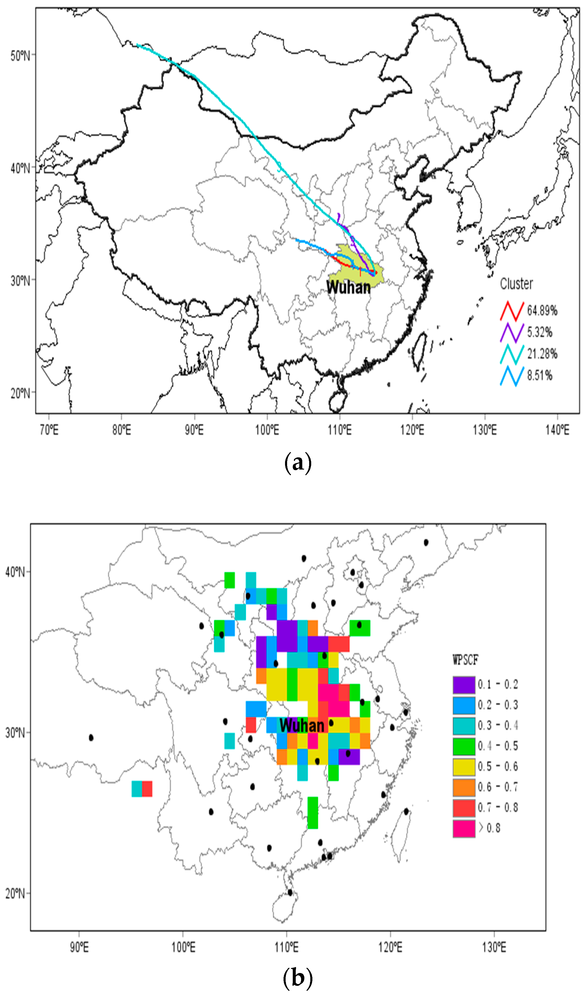
Additionally, cluster mean back trajectory result for Wuhan in December 2015 show that, polluted air masses from Sichuan, Chongqing, and southern Shaanxi accounted for 65% of all the trajectories (Figure 4a). Polluted air masses from Mongolia and through Ningxia and Henan accounted for 21% while other masses which were less important came from Gansu (9%) and Shaanxi (5%). Since cluster analysis cannot stimulate the values of daily PM2.5 levels caused by PSA [45], further analyses were done by using PSCF and CWT. Figure 4b shows the results of PSCF analysis where the pink color represents a high contribution level of PSA while the blue color represents low contribution of PM2.5 concentration. From the map, higher WPSCF values of above 0.5 are found in Gansu, Shaanxi, Shanxi, and more than 0.8 is seen in Henan province. These results suggest that these places were the PSA of pollutants in December. Moreover, results from the CWT method (Figure 4c) were very similar to the results obtained from the PSCF method. The highest values of WCWT are distributed over Anhui, Hebei, Henan, Gansu, Shaanxi, and Shanxi province corresponding with main contribution sources identified by the PSCF method. These areas have an important influence on PM2.5 concentration in Wuhan as the trajectories from these areas were the main contributor (100 µg/m3~187 µg/m3). Thus, these results signify that, apart from the condition of ABL, trans-boundary movement of air masses plays a significant role in determining the air quality of Wuhan city.
3.4. Analysis of O3 Pollution Event
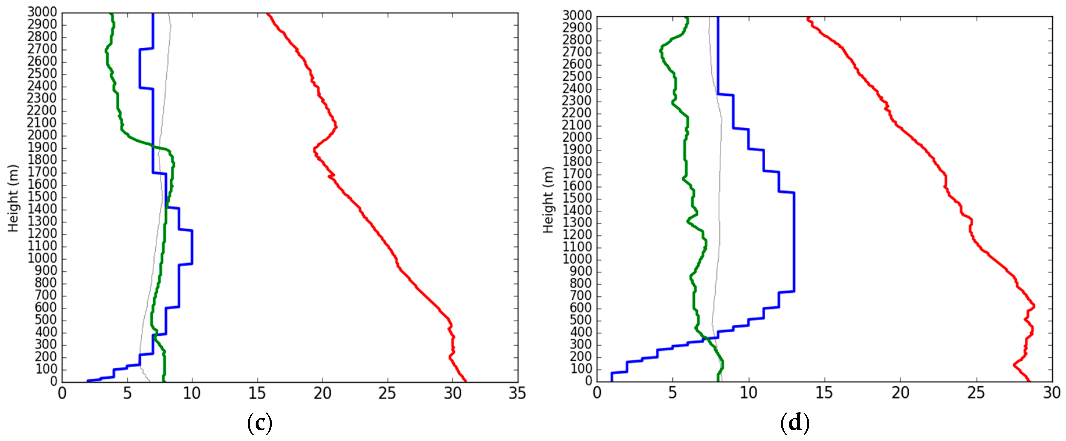
The averaged ABL structure of J-J-A for clean air which was composed of a total number of 31 days (Figure S2a) and the polluted air which was composed of a total number of 61 days (Figure S2b) show a slight difference in the speed of wind above an altitude of 100 m. During periods of significant air pollution, the wind speed at 600 m was around 6 m/s, the screen temperature was 27 °C and decreased with height at a rate of 0.4 °C/100 m in the lowest 600 m. Periods with clean air were characterized by a higher wind speed (9 m/s at 600 m), screen temperature (24 °C ), and slightly larger lapse rate, 0.5 °C/100 m. The direct influence of temperature on ozone production, through the speeding up of the rate of chemical reaction, which is thought to be the reason here, was discussed well by Coates et al. [46]. Similarly, a study by Kuang et al. [47] showed that Tropospheric ozone is strongly anticorrelated with relative humidity and strongly correlated with temperature. These general characteristics on polluted days are favorable for photochemical production of ozone and accumulation while conditions on the clean days are unfavorable for ozone accumulation due to high speed winds which can easily disperse pollutants, and low temperature which limit photochemical reactions. The daily average concentration of ozone for three months, J-J-A shows a periodic pattern with ‘peaks’ and ‘troughs’ (Figure 2). The ‘peaks’ are thought to be the results of continous accumulation of O3, while the ‘troughs’are thought to be the result of rainfall caused by the summer monsoon. Moreover, a clear O3 pollution event can be seen from 19 to 30 July, when its concentration accumulated for 10 days before it declined for two days (Figure 2). 19, 20, and 21 July recorded an AQI of below 50 which indicates that the quality of the air during these days was ‘excellent’ (Table 1), and average concentrations of ozone were 70 µg/m3, 93 µg/m3, and 144 µg/m3, respectively, which are all below the set standards of 160 µg/m3. It is thought that these three days (19–21 July) recorded excellent air conditions because they received rainfall of 58 mm, 18 mm, and below 0.1 mm, and the sunshine hours were 0 h, 0 h, and 10.4 h, respectively (Table S1). Note that, rainfall and high water vapor content [21] have the tendancy of inhibiting O3 formation by washing out ozone precursors and decreasing photolysis rates. Similar results to this have been reported by Ran et al. [2] in Shanghai as they found out that frequent rainfall significantly affects ozone concentration. Likewise, over these days, the wind speed at the ground was about 4 m/s which is not a favorable condition for pollutant accumulation, and there was no sunshine in the first two days (19 and 20 July). Note that the formation of O3 by photochemical reaction depends very much on the presence of solar radiation, so the absence of it inhibits ozone formation [20,23,30]. Moreover, the ABL structures on these days appeared to be very humid, especially on 19 and 20 July (Figure S3a,b), and slightly humid on 21 July (Figure S3c), when there was slight rainfall (Table S1). Average ground meteorological variables during the ozone pollution, and the average temperature over these three days was about 26.8 °C without ground inversion (Table S2). Significant changes in the ABL started to appear on 22 and 23 July (Figure S3d,e), when the screen temperature started to rise (Table S2) and the relative humidity dropped to about 60%. These changes can also be seen on the AQI as it was raised to 60 and 70, which suggest that the air quality was ‘good’ on 22 and 23 July when the average concentartions of ozone were 168 µg/m3 and 176 µg/m3, respectively. Over these two days, there was no rainfall recorded and the average sunshine hours was 11.7 h (Table S1). The observed higher concentration of ozone is thought to be the result of high temperature, extended sunshine hours, and the absence of rainfall. Comperable results were reported in previous studies by Shan et al. [30] and Coates et al. [46]. Suspended inversion layers developed and persisted on July 24, 25, 26, 27, and 28 of about 0.5 °C/100 m, 1.3 °C/100 m, 1.1 °C/100 m, 0.8 °C/100 m, and 0.4 °C/100 m, respectively (Figure S3f and Figure 5a–d). Moreover, sunshine hours on 24–28 July were 11.8 h, 12.2 h, 12.1 h, 11.5 h, and 11.2 h, respectively (Table S1). As it was pointed out earlier, solar radiation is an important factor in photochemical reactions, especially in the formation of ozone from nitrogen oxides and volatile organic compounds [22]. Over these five days (24–28 July), the AQI and concentration of ozone were also rising and reached their maximum levels at the peak of the pollution process, that is on 28 July 2016. The concentration of ozone on the peak day was 208 µg/m3 and the AQI was 110 which indicate that the quality of air was ‘slighly polluted’ (Table 1). ABL structure and back trajectory (Figure S4a–c) results show that the origin of the air masses during the whole process was mainly from southwest China, the region which has serious ozone pollution [5,16] partially due to the presence of heavy industries [3]. In addition to these air masses which were observed to come from the southwest throughout the pollution process, the peak of the pollution (28 July) received air masses from the southeast China sea (Figure S4d), the area which was reported by Tong et al. [20] as the PSA of ozone for eastern China. The continuous increase of the O3 observed during the whole pollution process is thought to be the result of pollutant accumulation, while sufficient sunshine hours facilitated the photochemical formation of ozone. Moreover, the development of an inversion layer and the presence of low wind speeds appeared to limit the vertical and horizontal dispersion of this pollutant. Similarly, cluster analysis for July, Figure 6a, shows that mean back trajectory from south China sea through Guangdong and Hunan contributed 34% followed by the one from Guangxi crossed through Hunan which accounted for 31% of all the trajectories. Trajectories from Jiangxi and the east China sea accounted for 24% and 12%, respectively. Furthermore, a map of PSCF shows the area with high values of WPSCF over Guangdong, Guangxi, Jianxi, Hunan, Anhui, and Shanghai (Figure 6b). Corroborated results of this were reported in a study by Gong et al. [16]. Therefore, these results indicate that these areas are important contributing sources of trans-boundary O3 in Wuhan.
4. Conclusions
This study analyzed six monitored air pollutants in Wuhan city which are used to determine the AQI together with the ABL structure, ground meteorological variables, and backward trajectory. The results show that the city was polluted in this study period during winter by PM2.5 and during summer by ozone. For the whole year, the highest AQI was 330 on 25 December 2015 which indicates ‘severe pollution’, and the lowest AQI was 27 on 26 August 2016, which indicates ‘excellent’ air quality. The percentage of days for the whole year with ‘excellent’, ‘good’, ‘slightly polluted’, ‘moderately polluted’, ‘heavily polluted’, and ‘severely polluted’ air were 13%, 52%, 24%, 7%, 3%, and 1%, respectively. Moreover, the annual average levels of PM2.5 and PM10 were 59 µg/m3 and 94 µg/m3, which are far above the NAAQS of 35 µg/m3 and 70 µg/m3, and the AQGs by the WHO of about 10 µg/m3 and 20 µg/m3, respectively. Evident pollution processes were observed for both PM2.5 and ozone pollution with different evolution characteristics at the ABL. During the PM2.5 pollution process, the ABL was observed to be dry, with a strong inversion layer and stagnant wind. These conditions favor pollutant accumulation and inhibit horizontal and vertical distribution of pollutants. Backward trajectories show the trans-boundary movement of air masses from the northwest, the area which is well-known for serious PM2.5 pollution. During the ozone pollution process, the ABL structure was found to be warm and the temperature decreased very slowly, with zero recorded rainfall, long sunshine duration, and a strong suspended inversion layer. These conditions are thought to be important for photochemical reactions. Moreover, a calm wind was observed during the pollution process, which facilitated the accumulation of pollutants. Backward trajectories show that there was a continous accumulation of pollutants thoughout the pollution process. Results in both scenarios suggest the trans-boundary movement of air masses to be an important factor in determining the air quality of Wuhan.
Supplementary Materials
Supplementary materials can be found at https://www.mdpi.com/2073-4433/9/9/359/s1.
Author Contributions
Conceptualization, Y.M. and J.Q.; Methodology, Y.M. and J.Q.; Software, Z.Y., Y.M. and J.H.; Validation, Z.Y., J.Q., J.H. and Y.M.; Formal Analysis, Y.M. and Z.Y; Investigation, Y.M.; Resources, J.Q.; Data Curation, J.H.; Writing-Original Draft Preparation, Y.M.; Writing-Review & Editing, Y.M.; Visualization, J.Q. and Y.M.; Supervision, J.Q.; Project Administration, J.Q.; Funding Acquisition, J.Q.
Funding
This study was supported by the National Key Research and Development Program of China (2016YFA0602002 and 2017YFC0212603).
Acknowledgments
Thanks to NOAA Air Resources Laboratory (ARL) for the provision of the HYSPLIT transport and dispersion model and/or READY website (http://www.ready.noaa.gov) used in this manuscript and Wuhan Environmental Protection Agency (WHEPA) and Wuhan Meteorological Bureau (WMB). Special thanks go to three anonymous reviewers for constructive comments and suggestions.
Conflicts of Interest
The authors declare no conflict of interest.
References
- World Health Organization (WHO). Ambient Air Pollution: A Global Assessment of Exposure and Burden of Diseases. 2016. Available online: http://apps.who.int/iris/bitstream/handle/10665/250141/?sequence=1 (accessed on 12 May 2018).
- Ran, L.; Zhao, C.; Geng, F.; Tie, X.; Tang, X.; Peng, L.; Zhou, G.; Yu, Q.; Xu, J.; Guenther, A. Ozone photochemical production in urban Shanghai, China: Analysis based on ground level observations. J. Geophys. Res. 2009, 114, 1–14. [Google Scholar] [CrossRef]
- Li, G.; Bei, N.; Cao, J.; Wu, J.; Long, X.; Feng, T.; Dai, W.; Liu, S.; Zhang, Q. Widespread and persistent ozone pollution in eastern China during the non-winter season of 2015: Observations and source attributions. Atmos. Chem. Phys. 2017, 17, 2759–2774. [Google Scholar] [CrossRef]
- Feng, Z.; Hu, E.; Wang, X.; Jiang, L.; Liu, X. Ground-level O3 pollution and its impacts on food crops in China: A review. Environ. Pollut. 2015, 199, 42–48. [Google Scholar] [CrossRef] [PubMed] [Green Version]
- Liu, T.; Tian, T.; Hui, Y.; Jun, Y.; Qian, X.; Yan, H.; Rong, Z.; Jun, W. The short-term effect of ambient ozone on mortality is modified by temperature in Guangzhou, China. Atmos. Environ. 2013, 76, 59–67. [Google Scholar] [CrossRef]
- People’s Republic of China National Ambient Air Quality Standard, China. 2012. Available online: http://210.72.1.216:8080/gzaqi/Document/gjzlbz.pdf (accessed on 8 March 2018). (In Chinese).
- World Health Organization (WHO). WHO Air quality Guidelines for Particulate Matter, Ozone, Nitrogen Dioxide and Sulfur Dioxide. Available online: http://apps.who.int/iris/bitstream/handle/10665/69477/WHO_SDE_PHE_OEH_06.02_eng.pdf?sequence=1 (accessed on 12 May 2018).
- Zhang, B.; Zhao, J.; Yang, R.; Qian, Z.; Liang, S.; Bassig, B.A.; Zhang, Y.; Hu, K.; Xu, S.; Dong, G.; et al. Ozone and Other Air Pollutants and the Risk of Congenital Heart Defects. Sci. Rep. 2016, 6, 34852. [Google Scholar] [CrossRef] [PubMed] [Green Version]
- Lyu, X.P.; Wang, Z.W.; Cheng, H.R.; Zhang, F.; Zhang, G.; Wang, X.M.; Ling, Z.H.; Wang, N. Chemical characteristics of submicron particulates (PM1.0) in Wuhan, Central China. Atmos. Res. 2015, 161, 169–178. [Google Scholar] [CrossRef]
- Song, J.; Guang, W.; Li, L.; Xiang, R. Assessment of air quality status in Wuhan, China. Atmosphere 2016, 7, 56. [Google Scholar] [CrossRef]
- Lyu, X.P.; Chen, N.; Guo, H.; Zeng, L.; Zhang, W.; Shen, F.; Quan, J.; Wang, N. Chemical characteristics and causes of airborne particulate pollution in warm seasons in Wuhan, central China. Atmos. Chem. Phys. 2016, 16, 10671–10687. [Google Scholar] [CrossRef]
- Qian, Z.; Liang, S.; Yang, S.; Trevathan, E.; Huang, Z.; Yang, R.; Wang, J.; Hu, K.; Zhang, Y.; Vaughn, M.; et al. Ambient air pollution and preterm birth: A prospective birth cohort study in Wuhan, China. Int. J. Hyg. Environ. Health 2016, 219, 195–203. [Google Scholar] [CrossRef] [PubMed]
- Lyu, X.P.; Chen, N.; Guo, H.; Zhang, W.H.; Wang, N.; Wang, Y.; Liu, M. Ambient volatile organic compounds and their effect on ozone production in Wuhan, central China. Sci. Total Environ. 2016, 541, 200–209. [Google Scholar] [CrossRef] [PubMed]
- Mbululo, Y.; Qin, J.; Yuan, Z.X. Evolution of atmospheric boundary layer structure and its relationship with air quality in Wuhan, China. Arab. J. Geosci. 2017, 10, 1–12. [Google Scholar] [CrossRef]
- Acciai, C.; Zhang, Z.; Wang, F.; Zhong, Z.; Lonati, G. Characteristics and Source Analysis of Trace Elements in PM2.5 in the Urban Atmosphere of Wuhan in Spring. Aerosol Air Qual. Res. 2017, 17, 2224–2234. [Google Scholar] [CrossRef]
- Gong, X.; Hong, S.; Jaffe, D.A. Ozone in China: Spatial Distribution and Leading Meteorological Factors Controlling O3 in 16 Chinese Cities. Aerosol Air Qual. Res. 2018, 18, 2287–2300. [Google Scholar] [CrossRef] [Green Version]
- Xu, G.; Jiao, L.; Zhang, B.; Zhao, S.; Yuan, M.; Gu, Y.; Liu, J. Spatial and Temporal Variability of the PM2.5/PM10 Ratio in Wuhan, Central China. Aerosol Air Qual. Res. 2017, 17, 741–751. [Google Scholar] [CrossRef] [Green Version]
- Wang, S.; Yu, S.; Yan, R.; Zhang, Q.; Li, P.; Wang, L.; Liu, W.; Zheng, X. Characteristics and origins of air pollutants in Wuhan, China, based on observations and hybrid receptor models. J. Air Waste Manag. Assoc. 2017, 67, 739–753. [Google Scholar] [CrossRef] [PubMed]
- Lu, X.; Chen, N.; Wang, Y.; Cao, W.; Zhu, B.; Yao, T.; Fung, J.C.H.; Lau, A.K.H. Radical Budget and Ozone Chemistry during Autumn in the Atmosphere of an Urban Site in Central China. J. Geophys. Res. 2017, 122, 3672–3685. [Google Scholar] [CrossRef]
- Tong, L.; Zhang, J.; Xiao, H.; Cai, Q.; Huang, Z. Identification of the potential regions contributing to ozone at a coastal site of eastern China with air mass typology. Atmos. Pollut. Res. 2017, 8, 1044–1057. [Google Scholar] [CrossRef]
- Zhang, L.; Jaffe, D.A. Trends and sources of ozone and sub-micron aerosols at the Mt. Bachelor Observatory (MBO) during 2004–2015. Atmos. Environ. 2017, 165, 143–154. [Google Scholar] [CrossRef]
- Gioda, A.; Oliveira, R.C.G.; Cunha, C.L.; Corrêa, S.M. Understanding ozone formation at two islands of Rio de Janeiro, Brazil. Atmos. Pollut. Res. 2018, 9, 278–288. [Google Scholar] [CrossRef]
- Jenkin, M.E.; Clemitshaw, K.C. Ozone and other secondary photochemical pollutants: Chemical processes governing their formation in the planetary boundary layer. Atmos. Environ. 2000, 34, 2499–2527. [Google Scholar] [CrossRef]
- Wang, T.; Cheung, V.T.F.; Anson, M.; Li, Y.S. Ozone and related gaseous pollutants in the boundary layer of eastern China: Overview of the recent measurement at a rural site. Geophys. Res. Lett. 2001, 28, 2373–2376. [Google Scholar] [CrossRef]
- Wan, W.; Xie, X.; Zhang, S. Health Effect Valuation of Ground-level Ozone Control in Beijing and its surrounding areas, China. Adv. Mater. Res. 2012, 360, 585–589. [Google Scholar] [CrossRef]
- Tao, Y.; Huang, W.; Huang, X.; Zhong, L.; Lu, S.; Li, Y.; Dai, L.; Zhang, Y. Estimated Acute Effects of Ambient Ozone and Nitrogen Dioxide on Mortality in the Pearl River Delta of Southern China. Environ. Health Perspect. 2012, 120, 393–398. [Google Scholar] [CrossRef] [PubMed] [Green Version]
- Wang, T.; Xue, L.; Brimblecombe, P.; Fat, Y.; Li, L.; Zhang, L. Ozone pollution in China: A review of concentrations, meteorological influences, chemical precursors, and effects. Sci. Total Environ. 2017, 575, 1582–1596. [Google Scholar] [CrossRef] [PubMed]
- Liu, F.; Wang, X.; Zhu, Y. Assessing current and future ozone-induced yield reductions for rice and winter wheat in Chongqing and the Yangtze River Delta of China. Environ. Pollut. 2009, 157, 707–709. [Google Scholar] [CrossRef] [PubMed] [Green Version]
- Feng, Z.; Sun, J.; Wan, W.; Hu, E.; Calatayud, V. Evidence of widespread ozone-induced visible injury on plants in Beijng China. Environ. Pollut. 2014, 193, 296–301. [Google Scholar] [CrossRef] [PubMed]
- Shan, W.; Yin, Y.; Lu, H.; Liang, S. A meteorological analysis of ozone episodes using HYSPLIT model and surface data. Atmos. Res. 2009, 4, 767–776. [Google Scholar] [CrossRef]
- Tang, G.; Zhu, X.; Xin, J.; Hu, B.; Song, T.; Sun, Y.; Zhang, J.; Wang, L.; Cheng, M.; Chao, N.; et al. Modelling study of boundary-layer ozone over northern China—Part I: Ozone budget in summer. Atmos. Res. 2017, 187, 128–137. [Google Scholar] [CrossRef]
- Hu, X.M.; Ma, Z.; Lin, W.; Zhang, H.; Hu, J.; Wang, Y.; Xu, X.; Fuentes, J.D.; Xue, M. Impact of the Loess Plateau on the atmospheric boundary layer structure and air quality in the North China Plain: A case study. Sci. Total Environ. 2014, 499, 228–237. [Google Scholar] [CrossRef] [PubMed]
- Wu, M.; Wu, D.; Fan, Q.; Wang, B.M.; Li, H.W.; Fan, S.J. Observational studies of the meteorological characteristics associated with poor air quality over the Pearl River Delta in China. Atmos. Chem. Phys. 2013, 13, 10755–10766. [Google Scholar] [CrossRef] [Green Version]
- Li, X.; Wang, Y.; Zhao, H.; Hong, Y.; Liu, N.; Ma, Y. Characteristics of Pollutants and Boundary Layer Structure during Two Haze Events in Summer and Autumn 2014 in Shenyang, Northeast China. Aerosol Air Qual. Res. 2018, 18, 386–396. [Google Scholar] [CrossRef] [Green Version]
- HJ 633-2012. Technical Requirements for Ambient Air Quality Index (AQI) (Trial Implementation), China. 2012, pp. 1–6. Available online: http://210.72.1.216:8080/gzaqi/Document/aqijsgd.pdf (accessed on 22 May 2018). (In Chinese).
- Dimitriou, K. The Dependence of PM Size Distribution from Meteorology and Local-Regional Contributions, in Valencia (Spain)—A CWT Model Approach. Aerosol Air Qual. Res. 2015, 15, 1979–1989. [Google Scholar] [CrossRef]
- Rolph, G.D. READY Real-time Environmental Applications and Display System. Available online: http://www.ready.noaa.gov (accessed on 14 May 2018).
- Stein, A.F.; Draxler, R.R.; Rolph, G.D.; Stunder, B.J.B.; Cohen, M.D.; Ngan, F. NOAA’s HYSPLIT atmospheric transport and dispersion modeling system. Bull. Am. Meteorol. Soc. 2015, 96, 2059–2077. [Google Scholar] [CrossRef]
- Zeng, Y.; Hopke, P.K. A Study of the Sources and Acid Precipitation in Ontario, Canada. Atmos. Environ. 1989, 23, 1499–1509. [Google Scholar] [CrossRef]
- Polissar, A.V.; Hopke, P.K.; Paatero, P.; Kaufmann, Y.J.; Hall, D.K.; Bodhaine, B.A.; Dutton, E.G.; Harris, J.M. The aerosol at Barrow, Alaska: Long-term trends and source locations. Atmos. Environ. 1999, 33, 2441–2458. [Google Scholar] [CrossRef]
- Wang, Y.Q.; Zhang, X.Y.; Draxler, R.R. TrajStat: GIS-based software that uses various trajectory statistical analysis methods to identify potential sources from long-term air pollution measurement data. Environ. Model. Softw. 2009, 24, 938–939. [Google Scholar] [CrossRef]
- Lu, Z.; Streets, D.G.; Zhang, Q.; Wang, S.; Carmichael, G.R.; Cheng, Y.F.; Wei, C.; Chin, M.; Diehl, T.; Tan, Q. Sulfur dioxide emissions in China and sulfur trends in East Asia since 2000. Atmos. Chem. Phys. 2010, 10, 6311–6331. [Google Scholar] [CrossRef] [Green Version]
- Zhang, Z.; Wang, W.; Cheng, M.; Liu, S.; Xu, J.; He, Y.; Meng, F. The contribution of residential coal combustion to PM 2.5 pollution over China’s Beijing-Tianjin-Hebei region in winter. Atmos. Environ. 2017, 159, 147–161. [Google Scholar] [CrossRef]
- Cai, Z.; Jiang, F.; Chen, J.; Jiang, Z.; Wang, X. Weather Condition Dominates Regional PM2.5 Pollutions in the Eastern Coastal Provinces of China during Winter. Aerosol Air Qual. Res. 2018, 18, 969–980. [Google Scholar] [CrossRef] [Green Version]
- Xin, Y.; Wang, G.; Chen, L. Identification of Long-Range Transport Pathways and Potential Sources of PM10 in Tibetan Plateau Uplift Area: Case Study of Xining, China in 2014. Aerosol Air Qual. Res. 2016, 16, 1044–1054. [Google Scholar] [CrossRef] [Green Version]
- Coates, J.; Mar, K.A.; Ojha, N.; Butler, T.M. The influence of temperature on ozone production under varying NOx conditions—A modelling study. Atmos. Chem. Phys. 2016, 11601–11615. [Google Scholar] [CrossRef]
- Kuang, S.; Newchurch, M.J.; Thompson, A.M.; Stauffer, R.M.; Johnson, B.J.; Wang, L. Ozone Variability and Anomalies Observed During SENEX and SEAC4RS Campaigns in 2013. J. Geophys. Res. Atmos. 2017, 122, 11227–11241. [Google Scholar] [CrossRef] [PubMed]
Figure 1.
Daily average concentration of PM2.5 (particulate matter with aerodynamics of less than 2.5 microns) and air quality index (AQI) from 1 December 2015 to 29 February 2016. The red line shows the demarcation of days which are below and above daily acceptable limit of PM2.5.
Figure 1.
Daily average concentration of PM2.5 (particulate matter with aerodynamics of less than 2.5 microns) and air quality index (AQI) from 1 December 2015 to 29 February 2016. The red line shows the demarcation of days which are below and above daily acceptable limit of PM2.5.

Figure 2.
Concentration of ozone and air quality index (AQI) from 1 June 2016 to 31 August 2016. The red line shows the demarcation of days which are below and above daily acceptable limit of ozone.
Figure 2.
Concentration of ozone and air quality index (AQI) from 1 June 2016 to 31 August 2016. The red line shows the demarcation of days which are below and above daily acceptable limit of ozone.

Figure 3.
Vertical structure of the atmosphere on (a) 24 December 2015, AQI = 208; (b) 25 December 2015, AQI = 330; (c) 26 December 2015, AQI = 175; (d) 27 December 2015, AQI = 208 showing the profile of Temperature (red line, °C), relative humidity (green line, %), wind velocity (blue line, m/s), dominant wind direction (grey line) during the pollution process. The number on the X-axis is the result after dividing the relative humidity value by 10 and the wind direction angle by 30, while the temperature and wind speed remain the same.

Figure 4.
Maps showing (a) Cluster-mean back trajectories for December, (b) Spatial distribution of Weight Potential Source Contribution Function (WPSCF) (c) Spatial distribution of Weight Concentration Weighted Trajectory (WCWT).
Figure 4.
Maps showing (a) Cluster-mean back trajectories for December, (b) Spatial distribution of Weight Potential Source Contribution Function (WPSCF) (c) Spatial distribution of Weight Concentration Weighted Trajectory (WCWT).

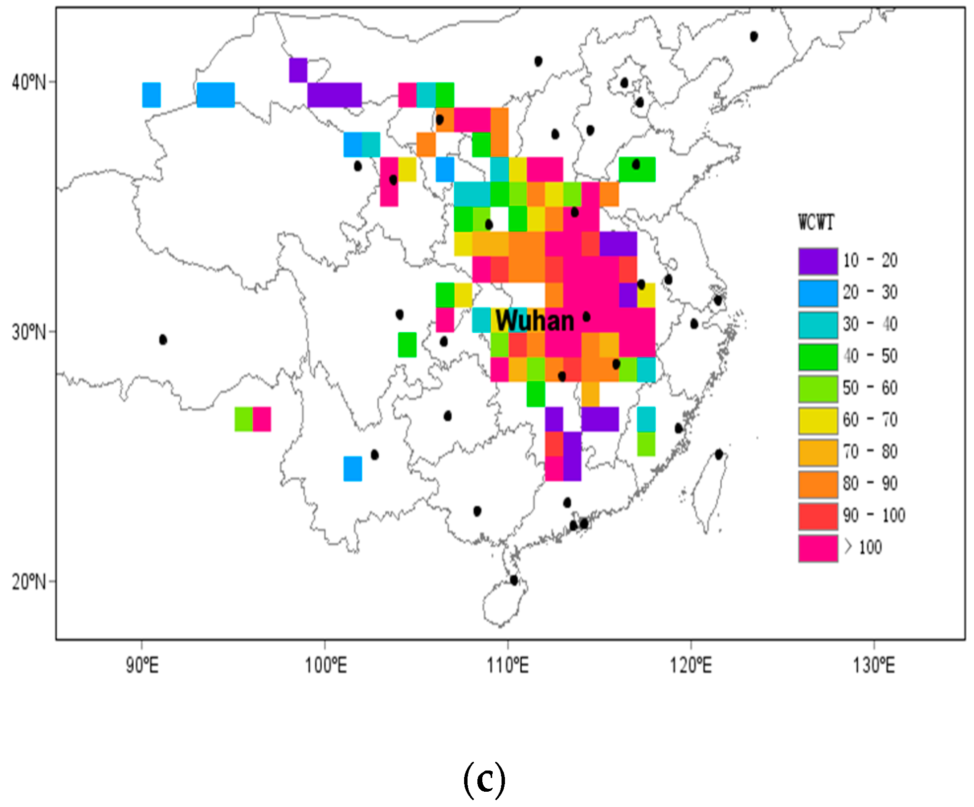
Figure 5.
Vertical structure of the atmosphere on (a) 25 July 2016, AQI = 91; (b) 26 July 2016, AQI = 95; (c) 27 July 2016, AQI = 99; (d) 28 July 2016, AQI = 110 showing the profile of Temperature (red line, °C), relative humidity (green line, %), wind velocity (blue line, m/s), dominant wind direction (grey line) during the pollution process. The number on the X-axis is the result after dividing the relative humidity value by 10 and the wind direction angle by 30, while the temperature and wind speed remain the same.
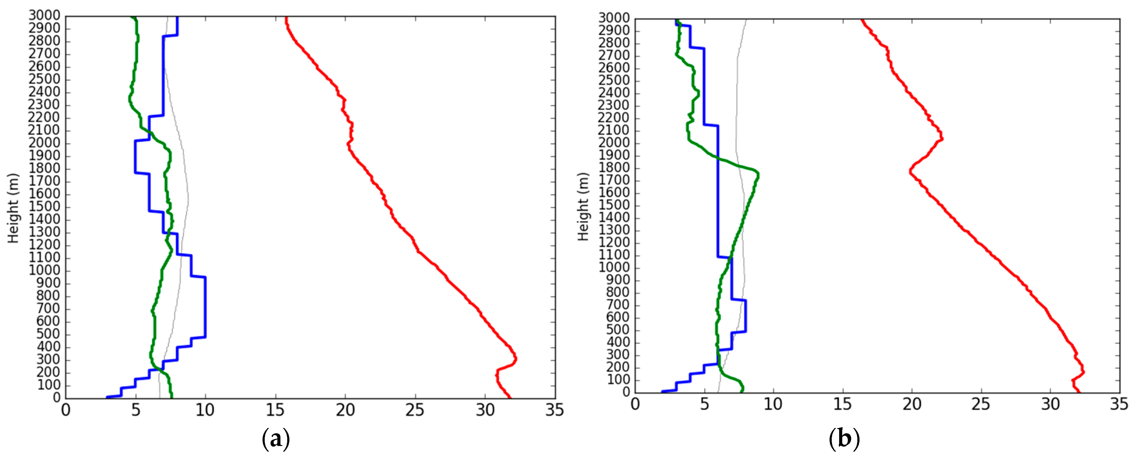

Figure 6.
Map showing (a) Cluster-mean trajectory result for July, (b) Spatial distribution of WPSCF.
Figure 6.
Map showing (a) Cluster-mean trajectory result for July, (b) Spatial distribution of WPSCF.


Table 1.
China air quality grading standards.
| Air Quality Index (AQI) | Air Quality Index Level | Air Quality Index Category |
|---|---|---|
| 0~50 | Level 1 | Excellent |
| 51~100 | Level 2 | Good |
| 101~150 | Level 3 | Slightly polluted |
| 151~200 | Level 4 | Moderate polluted |
| 201~300 | Level 5 | Heavy pollution |
| >300 | Level 6 | Severe pollution |
Table 2.
Ground meteorological variables during the PM2.5 (particulate matter with aerodynamics of less than 2.5 microns) pollution process.
Table 2.
Ground meteorological variables during the PM2.5 (particulate matter with aerodynamics of less than 2.5 microns) pollution process.
| Date | Air Temperature (°C) | Humidity (%) | Wind Speed (m/s) | Wind Direction | Pressure (hPa) | Characteristics of Inversion Layer | ||
|---|---|---|---|---|---|---|---|---|
| Strength (°C/100 m) | Altitude (m) | Thickness (m) | ||||||
| 16 December 2015 | 1.1 | 66 | 3 | 360 | 1032 | 2.5 | 0 | 90 |
| 17 December 2015 | −3.0 | 96 | 1 | 315 | 1032 | 1.9 | 0 | 220 |
| 18 December 2015 | −3.0 | 97 | 2 | 113 | 1030 | 4.2 | 0 | 130 |
| 19 December 2015 | 4.2 | 66 | 1 | 45 | 1028 | 0.2 | 0 | 140 |
| 20 December 2015 | 4.0 | 85 | 1 | 248 | 1027 | NIL | NIL | NIL |
| 21 December 2015 | 5.4 | 90 | 2 | 90 | 1023 | NIL | NIL | NIL |
| 22 December 2015 | 5.5 | 97 | 2 | 360 | 1023 | 0.5 | 360 | 110 |
| 23 December 2015 | 5.2 | 93 | 2 | 68 | 1021 | 0.2 | 320 | 100 |
| 24 December 2015 | 5.6 | 97 | 2 | 360 | 1022 | NIL | NIL | NIL |
| 25 December 2015 | 0.3 | 98 | 0 | C | 1027 | 2.3 | 0 | 270 |
| 26 December 2015 | 2.2 | 97 | 3 | 158 | 1021 | 2.3 | 0 | 260 |
| 27 December 2015 | 3.0 | 94 | 2 | 338 | 1024 | 1.9 | 0 | 180 |
| 28 December 2015 | 2.7 | 90 | 1 | 360 | 1034 | 0.5 | 350 | 250 |
| Average | 2.6 | 89.7 | 1.7 | 360 | 1026 | 1.7 | 343m | 175 |
m Averaged suspended inversions below altitude of 600 m.
© 2018 by the authors. Licensee MDPI, Basel, Switzerland. This article is an open access article distributed under the terms and conditions of the Creative Commons Attribution (CC BY) license (http://creativecommons.org/licenses/by/4.0/).
Share and Cite
MDPI and ACS Style
Mbululo, Y.; Qin, J.; Hong, J.; Yuan, Z. Characteristics of Atmospheric Boundary Layer Structure during PM2.5 and Ozone Pollution Events in Wuhan, China. Atmosphere 2018, 9, 359. https://doi.org/10.3390/atmos9090359
AMA Style
Mbululo Y, Qin J, Hong J, Yuan Z. Characteristics of Atmospheric Boundary Layer Structure during PM2.5 and Ozone Pollution Events in Wuhan, China. Atmosphere. 2018; 9(9):359. https://doi.org/10.3390/atmos9090359
Chicago/Turabian StyleMbululo, Yassin, Jun Qin, Jun Hong, and Zhengxuan Yuan. 2018. "Characteristics of Atmospheric Boundary Layer Structure during PM2.5 and Ozone Pollution Events in Wuhan, China" Atmosphere 9, no. 9: 359. https://doi.org/10.3390/atmos9090359
Note that from the first issue of 2016, this journal uses article numbers instead of page numbers. See further details here.