Gap-Filling of MODIS Time Series Land Surface Temperature (LST) Products Using Singular Spectrum Analysis (SSA)

Abstract

Land surface temperature (LST) is a basic parameter in energy exchange between the land and the atmosphere, and is frequently used in many sciences such as climatology, hydrology, agriculture, ecology, etc. Time series of satellite LST data have usually deficient, missing, and unacceptable data caused by the presence of clouds in images, the presence of dust in the atmosphere, and sensor failure. In this study, the singular spectrum analysis (SSA) algorithm was used to resolve the problem of missing and outlier data caused by cloud cover. The region studied in the present research included an image frame of the Moderate Resolution Imaging Spectroradiometer (MODIS) with horizontal number 22 and vertical number 05 (h22v05). This image involved a large part of Iran, Turkmenistan, and the Caspian Sea. In this study, MODIS LST products (MOD11A1) were used during 2015 with approximately 1 km × 1 km spatial resolution and day/night LST data (daily temporal resolution). On average, the data have 36.37% gaps in each pixel profile with 730 day/night LST data. The results of the SSA algorithm in the reconstruction of LST images indicated a root mean square error (RMSE) of 2.95 Kelvin (K) between the original and reconstructed LST time series data in the study region. In general, the findings showed that the SSA algorithm using spatio-temporal interpolation can be effectively used to resolve the problem of missing data caused by cloud cover.

1. Introduction

Land surface temperature (LST) is a principal characteristic for the evaluation of energy exchange between the land and the atmosphere [1,2,3]. This parameter is applicable to numerous sciences such as climatology, hydrology, agriculture, ecology, public health, and the environment [4,5,6,7,8,9,10,11,12,13,14,15]. One of the methods for measuring LST is to use satellite data and thermal remote sensing techniques. However, time series of the satellite observations of LST often have missing data and outliers. Missing values and/or outliers can arise from cloud cover, sensor failure, aerosol, and the inefficiency of cloud-masking algorithms [1,2,16,17]. Atmospheric dust, aerosol, gases, and clouds in particular can dramatically affect the energy reflected from the surface and expose the reading of optical and thermal sensors to error [16]. Clouds in satellite images are identified as phenomena that have higher reflection in visible bands of the electromagnetic spectrum than most other terrestrial phenomena, and have a lower temperature than the below land surface in the thermal bands [18]. The clouds, which absorb part of the upwelling energy of the land surface and emit thermal infrared energy, exhibit relative lower temperature than the ground objects; thus, they are not correctly diagnosed in a cloud-masking algorithm. Consequently, some negative outliers, which show lower temperature than the other measurements, will remain in place of missing data in a time series [19]. Therefore, satellite imageries of LST covered by cloud have been a major limitation in choosing the images.

The missing data in a time series, depending on the size, dispersion, temporal distribution, and their continuity over time, can be very short, dispersed, or have a long gap. According to the continuity of the missing data time series, two terms can be defined: missing data with a short gap, and missing data with a long gap. When there are less than 50% of the sampled data over time, they are subject to missing data with a short gap/size in time series. However, if more than half of the sampled data are missing, this time series will have a large gap [20,21]. The outliers, whose values significantly deviate from normal changes in a dataset, can be classified into positive and negative data [19]. For example, values larger than one or smaller than −1 in a Normalized Difference Vegetation Index (NDVI) time series are errors and can be defined as outliers. Further, a sharp increase or decrease of NDVI data in a time series of NDVI, compared to the data before and after it, can be identified as outliers. Time series can be periodic or non-periodic. Remote sensing LST time series are included in periodic time series because they reflect the daily, seasonal, and multi-annual variations of the sun.

Several methods have been developed to identify cloud cover and fill in missing data, including the spectrum-based approach, which employs all of the spectral data to detect whether a specific pixel contains cloud; and the temporal-based approach, which presents an evaluation of the missing values caused by cloud cover through temporal interpolation [16]. For example, the fast Fourier transform (FFT) algorithm and harmonic analysis of time series (HANTS) algorithm that are used to reconstruct the missing data and remove the outliers in the time series of NDVI are based on the second approach [17,21,22,23,24,25]. The HANTS algorithm was first developed to reconstruct the NDVI time series and extract phenological data. However, since this algorithm reconstructs the signal of a time series based on periodic behavior, it was effectively used to reconstruct other time series with periodic behavior such as LST [2,19,26,27]. A disadvantage of HANTS is that in these methods, only temporal correlation between observations is used to fill the gap of missing data in a time series.

Singular spectrum analysis (SSA) is an advanced method that uses SSA (with only one time series) and multi-channel singular spectrum analysis (M-SSA for more than a time series) to reconstruct the time series with missing data, especially with a large gap. SSA was first developed by Broomhead and King (1986). It was then proposed by Vautard and Ghil (1992) and Kondrashov and Ghil (2006) to fill the gaps of missing data in a time series [28,29,30]. The value of each pixel in an LST image over time is the result of the interaction between radiation energy and ambient turbulent energy. Therefore, this time series has regular (cycle) and irregular (noise) components. Using this presumption, SSA makes use of empirical orthogonal functions (EOFs) and an analysis of major components in the temporal domain to extract data from short and noisy time series, without primary knowledge about the dynamic processes that affect these time series [30]. SSA is an advanced method for the analysis of a time series that makes use of multivariate principles of statistics, geometry, linear algebra, and signal processing [31]. SSA analyzes the time series to simpler and interpretable components such as trends, periodic and semi-periodic fluctuations, and noises [32]. Thus, several significant components achieve maximum variance, and noises achieve minimum variance in observations of a time series.

SSA has been used as a standard tool in the analysis of a climatic time series, meteorology, and geophysics [33,34,35,36,37]. Ghafarian et al. (2015) were reconstructed the hourly LST time series data using SSA and M-SSA. The results showed a mean absolute error of 2.25 °K in an hourly time series with 63% of the missing data caused by cloud cover [1]. In another study, the SSA algorithm was used to reconstruct the missing data in the leaf area index (LAI) of MODIS data. The findings indicated that M-SSA effectively reconstructed this index using spatio-temporal correlation [38]. Moreover, another study showed that SSA could be effective in an analysis of a hydrologic time series, including the reconstruction of time series and extraction of trends, fluctuations, and prediction [39].

The current study was aimed to (1) assess the performance of SSA and M-SSA algorithms in removing the clouds and outliers in a daily MODIS LST time series; and (2) reconstruct the cloud-free daily MODIS LST time series with validation. We hope that this study can be helpful and practical in pushing this researching domain forward, especially concerning climate change and associative hazard risks.

2. Study Area, Data

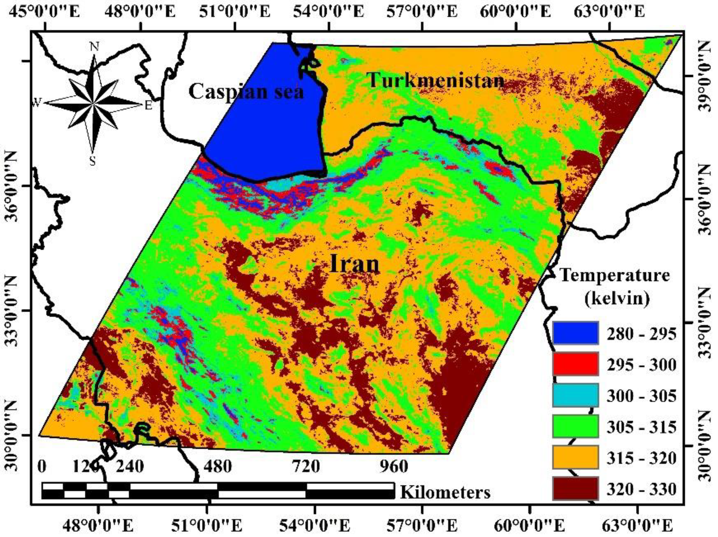
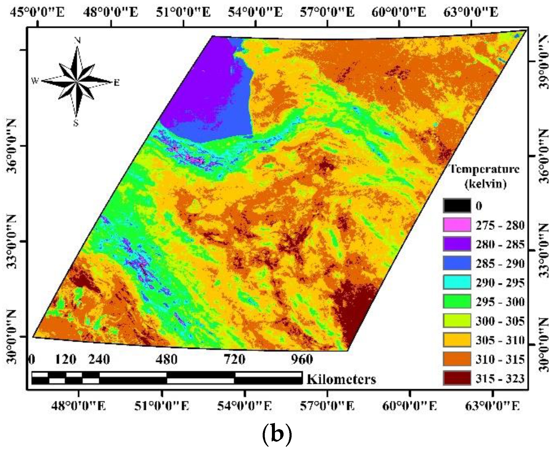
2.1. Study Area

The study region, which covers a large part of Iran, Turkmenistan, small fragments of Iraq, Uzbekistan, and the Caspian Sea, is located in the Middle East. The Caspian coastline, with a height of 28 m below sea level, is located at the north part of the study area, and the Alborz and Zagros mountain ranges (with a highest peak of 5610 m in Mount Damavand) are located at the western and northern parts of the study area, respectively. This vast area, together with severe topographical changes, has led to different vegetation coverage, from the vegetation-free areas (generally in the center of Iran) to areas with 100% vegetation coverage (southern Caspian Sea). The latitudes of the study area are between 30° N and 40° N and the longitudes are between 46°11′6″ E and 65°16′14″ E.

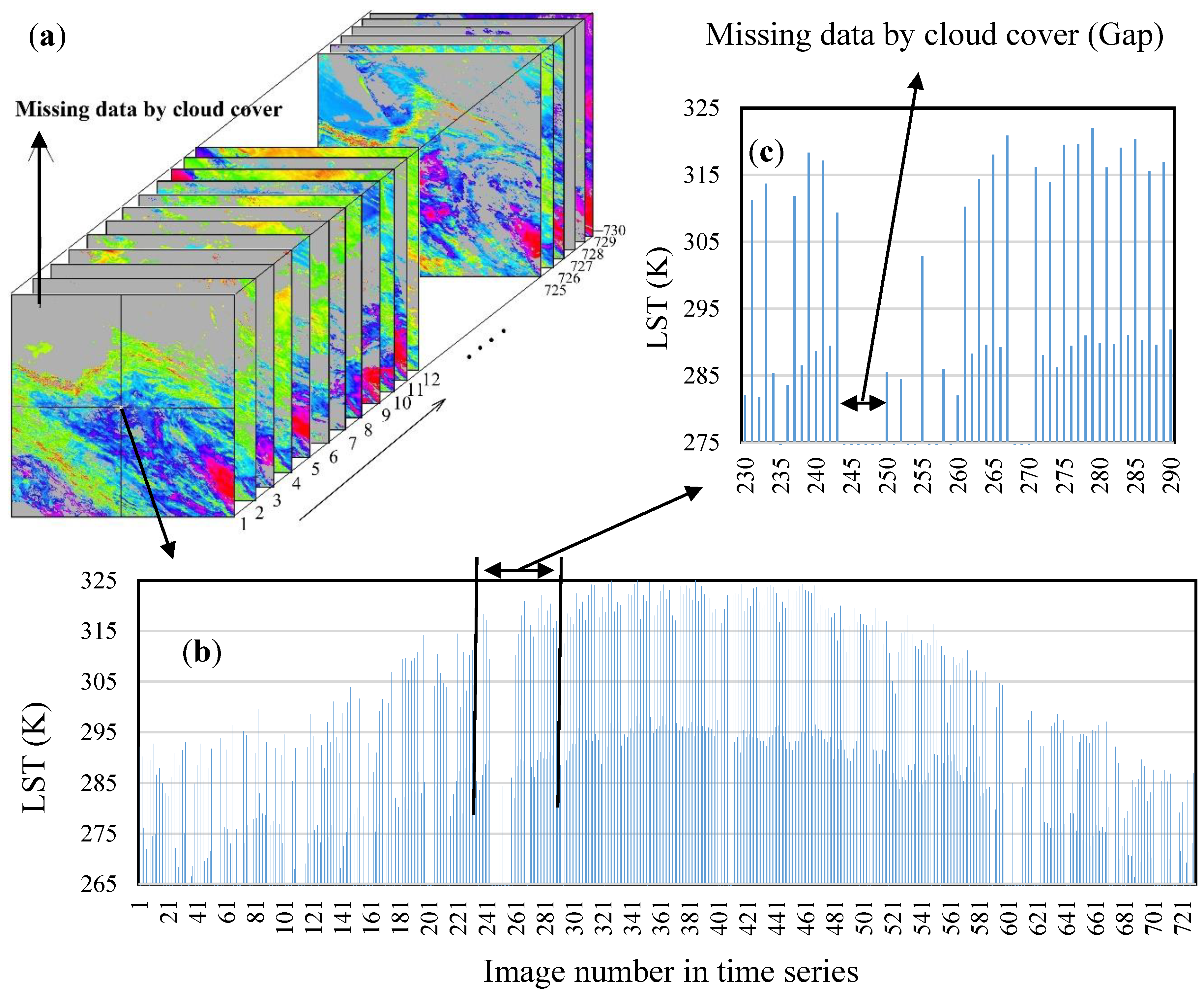
2.2. Data (Satellite Time Series Images)

The study region covers an image frame of the MODIS sensor (LST product) with horizontal number 22 and vertical number 5 (h22v5) in the MODIS sinusoidal tiling system. As an example, Figure 1 displays an LST image of the studied region in the Universal Transverse Mercator (UTM) coordinate system.

In this study, daily MODIS LST products (MODIS11A1) from the Terra satellite were used during 2015. The MOD11A1 product contains LST data from instantaneous measurements at specific hours of the day and night. Scan times are given in the local solar time in separate product layers named “Day_view_time” and “Night_view_time”. The spatial and temporal resolution are 1 km × 1 km (the exact grid size is 0.928 km by 0.928 km at a spatial resolution of 1 km) and daily (day and night), respectively.

This MODIS LST product were obtained from two thermal infrared bands of channels 31 (wavelength range of 10.78–11.28 µm) and 32 (wavelength range of 11.77–12.27 µm) using split-window algorithm 2 [5,40,41]. The annual LST time series in this study included 365 day and 365 night LST images. The LST images in the present study were considered as day/night sequences during the year. Hence, in this time series with 730 images, the odd numbers showed the LST images during the day, and the even numbers indicated the LST images at night. Images 1 and 2 are for 1 January, and images 729 and 730 are for 31 December. First, a time series with 730 LST images along with missing data due to the cloud cover is shown in Figure 2a,b, which depicts the LST changes along one pixel in this time series. For a sharper display in Figure 2c, a part of this time series is magnified.

3. Methodology

Singular Spectrum Analysis (SSA)

For sake of clarity, the SSA algorithm can be divided in four steps illustrated as follows based on Ghafarian et al. (2012) and Musial et al. (2011) [1,42]:

Step 1: Let’s have a single scalar time series x(t); with t = 1, 2, 3, …, n that is embedded into a multi-dimensional trajectory matrix of lagged vectors:

$$x=\left[x_1,\dots ,x_{n^{\prime }}\right]$$

(1)

where n′ = n − m + 1, and each lagged vector is defined as:

$$x_j={(x_j,\dots ,x_{j+m-1})}^T$$

(2)

This trajectory matrix contains the complete record of patterns presented within a window of size m. By selecting a large window size, more information about the basic pattern of the time series will be captured. A small window size value enhances the statistical confidence of the final results [43], since the structure of the time series will be captured repeatedly [44]. The final form of the trajectory matrix X is a rectangular matrix of the form:

$$X=\left(\begin{array}{ccc}{x}_1& x_2& x_3\\ x_2& x_3& x_4\\ x_3& x_4& x_5\\ \dots & \dots & \dots \\ x_m& x_{m+1}& x_{m+2}\end{array}\begin{array}{cc}\dots & x_k\\ \dots & x_{k+1}\\ \dots & x_{k+2}\\ \dots & \dots \\ \dots & x_n\end{array}\right)$$

(3)

Step 2: The next step is a decomposition of trajectory matrix X of size m × n′ using the singular value decomposition (SVD) method, which yields:

$$X=DL{E}^T$$

(4)

where D and E are the left and right singular vectors of X with m × m and n × n sizes, respectively, and L is a rectangular diagonal matrix of size m × n. The elements of L, which are called singular values, are the square roots of the eigenvalues of the lagged-covariance matrix S = XXT of size m × m. The columns of matrix D are the eigenvectors of S, and are also known as empirical orthogonal functions (EOFs). The rows of E^T are eigenvectors of matrix XTX. If we plot the singular values in descending order, one can often distinguish between an initial steep slope, representing a signal, and a (more or less) flat floor, representing the noise level [30]. Then, any subset of the d eigenvalues (EOFs), 1 ≤ d ≤ m, for which related eigenvalues are positive, provides the best representation of the matrix X as a sum of matrices X_i, i = 1, 2, …, d [32].

Step 3: Partitioning d eigentriples into p distinct subsets. Then, summing all of the components inside each subset such that:

$$X={\displaystyle \sum _{n^{\prime }=1}^p}{X}_{I_{n^{\prime }}}where,X_{I_{n^{\prime }}}={\displaystyle \sum _{i\epsilon I_{n^{\prime }}}{X}_i}$$

(5)

The matrices X_In′ have the form of a Hankel matrix in an ideal case, and consequently fit the trajectory matrices.

Step 4: Since the ideal case described in step 3 is not usually the case, the X_In′ matrices should be transformed into the form of a Hankel matrix to fit the trajectory matrices. This step is known as diagonal averaging. In this sense, the original matrix can be reconstructed as the sum of these matrices:

$$x_t={\displaystyle \sum _{n^{\prime }=1}^p{x_t}^{n^{\prime }}},t=0,1,\dots ,n-1$$

(6)

where for each p, the series x_t^n′ is the result of the diagonal averaging of the matrix X_In′.

The SSA workflow for the gap-filling procedure consists of several steps, which are explained as follows:

For a given window width (m), the original time series is centered by computing the unbiased value of the mean, and the missing data is set to zero. The first leading EOF is found by an iterative procedure that applies the SSA algorithm on the zeroed and centered set. The missing values are updated based on the reconstructed component of the current EOF. Using this updated set, the SSA algorithm is applied again, and the missing values are updated based on the result of this new iteration. The process repeats until convergence is achieved. Then, the iteration starts for the second leading EOF (keeping the first one fixed) until convergence has been achieved for the second EOF. This process repeats for the selected number of EOFs, each time keeping the previous ones as fixed. To find the optimal value for the window width and the number of dominant SSA modes to fill the gaps, cross-validation is applied. It means that a portion of the available data (selected as random) is flagged as missing, and the RMSE error from the reconstruction is computed to find the best value for the window size and number of EOFs. The SSA can only be applied on a single time series, but the SSA technique can be generalized to be used for a multivariate time series (applying on the multi-time series namely as, M-SSA, multi-singular spectrum analysis) and gap-filling the missing values in those time series [45].

In this research, the spatio-temporal dispersion of the missing data in time series is shown. The spatial dispersion is the same missing data caused by cloud cover in each time series image, and temporal distribution is the missing data along 730 images over time. To display the spatial dispersion of the missing data, the image statistics in ENVI 4.8 software were used. Also, to show the temporal distribution of the missing data, the missing data caused by cloud cover along each pixel of this time series were counted and then divided by the total number of data over time. Hence, the map of missing data in this time series was prepared.

SSA-MTM software was used to reconstruct the LST time series with 730 images during 2015. This software is accessible via http://research.atmos.ucla.edu/tcd//ssa/form.html for free. To reconstruct the time series in SSA software, it is necessary to determine the number of significant components and window size. As these components are the results of the movement of the sun and the seasonal and annual variation of LST, the whole LST observations over time are shown as those components. To determine these parameters, first, a single time series without missing data was selected as a representative of the whole time series. Then, the effects of window size and the number of components in the reconstruction of this time series were assessed by SSA. Next, the significant components were determined by different tests in SSA software such as the Monte Carlo test. This will be explained in further detail in the results section. Having determined the window size and significant components, the time series of all of the images were reconstructed by M-SSA using these results. It should be pointed out that due to the lengthy discussion of SSA software, tests such as the Monte Carlo test, as well as testing the null hypothesis of EOFs and a theoretical discussion on the trends and periods, more information can be found in the study of Ghafarian Malamiri (2015) [19].

To evaluate the M-SSA performance in reconstructing the images of this time series, the root mean square error (RMSE) was used, which is obtained from Equation (7). In this equation, x_i and y_i represent original and reconstructed data, respectively.

$$RMSE=\sqrt{\frac{{\displaystyle \sum _{i=1}^n{(x_i-y_i)}^2}}{n}}$$

(7)

To calculate the RMSE, firstly the cloud data, which means the data with zero value, was removed. Then, the RMSE was computed between the true data and reconstructed data by the SSA algorithm along each pixel of this time series, and displayed as an RMSE map.

4. Results

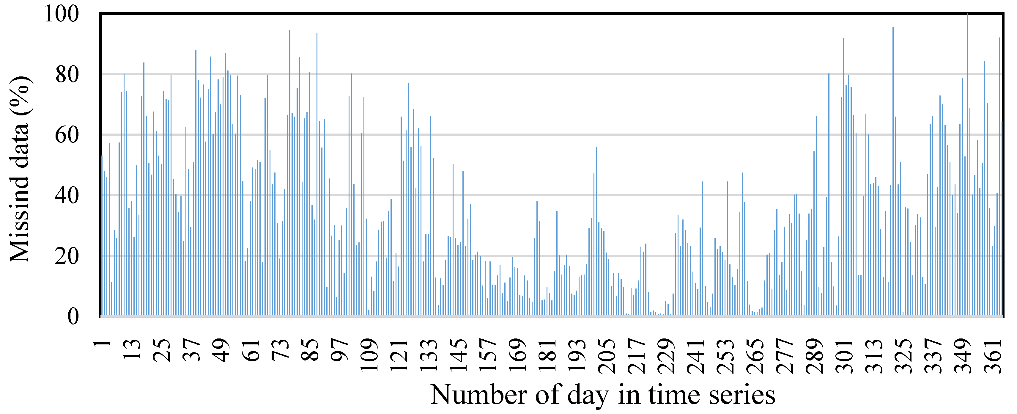
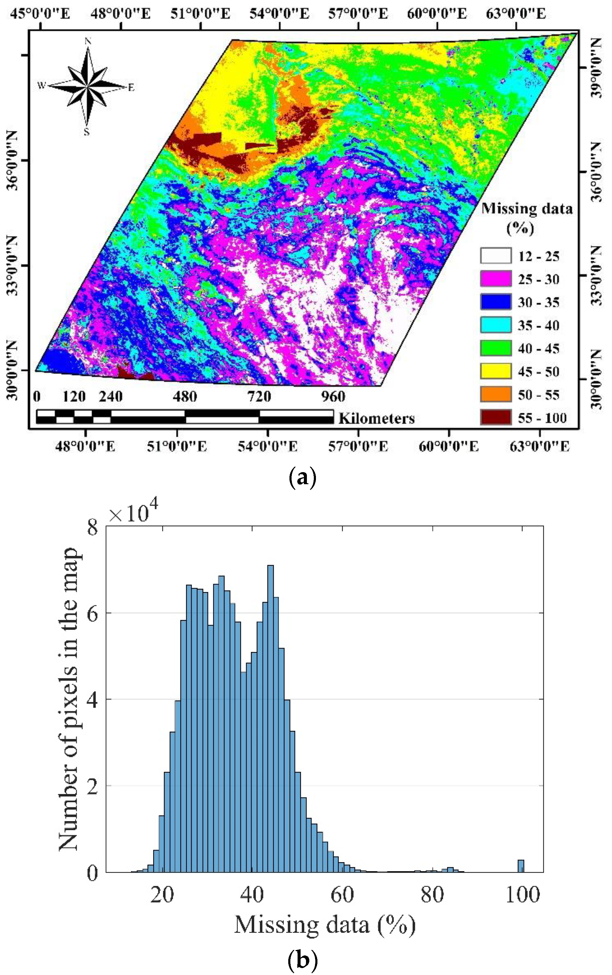
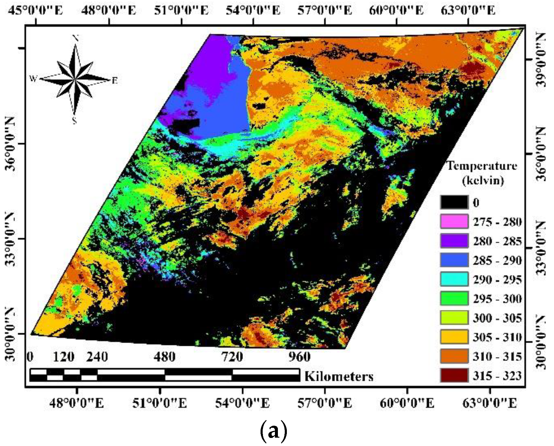
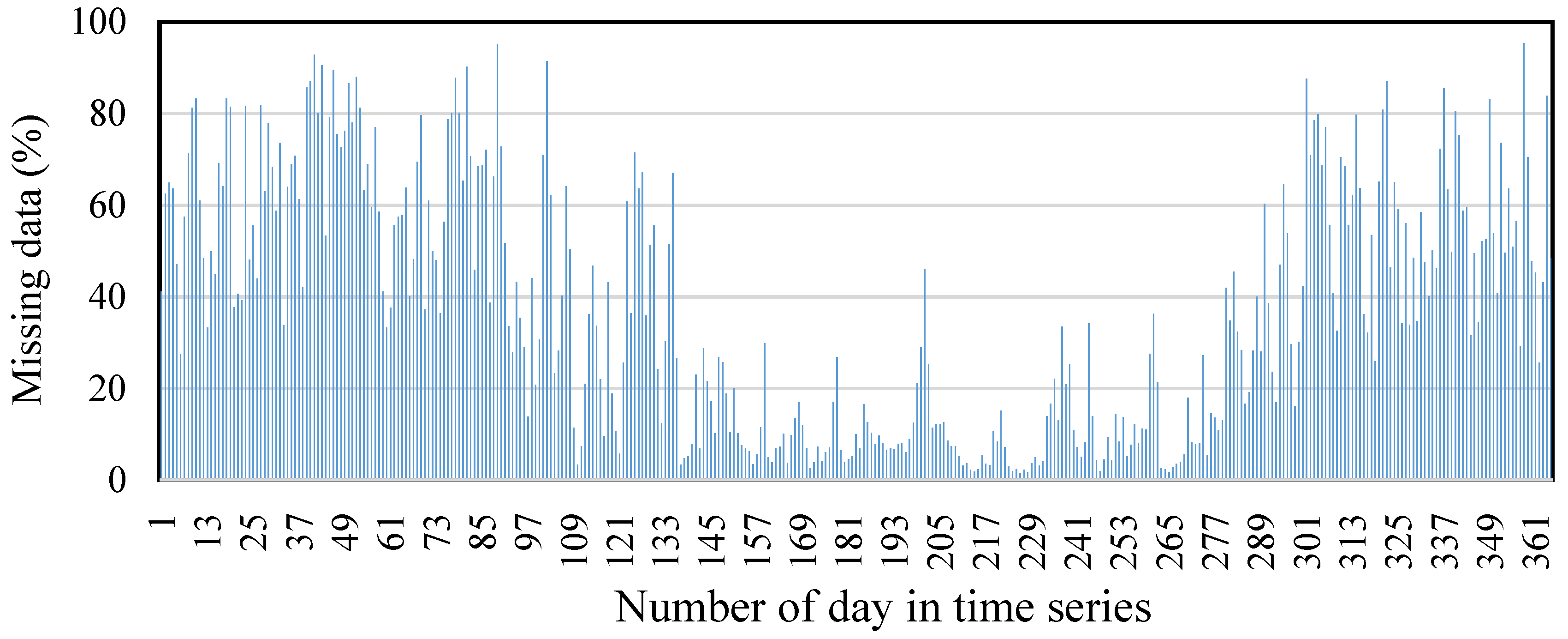
4.1. Spatio-Temporal Distribution of the Missing Data

To analyze the performance of the SSA algorithm in reconstructing LST images, the distribution style and amount of missing data in the LST time series were calculated temporally and spatially. For a better display, the time series with 730 images were depicted in the LST time series during the day and night. The percentages of missing data in each LST time series image (temporal dispersion) are shown during the day and at night in Figure 3 and Figure 4. On the horizontal axis (Figure 3), number one is related to 1 January 2015. Based on Figure 3 and Figure 4, the amount of missing data is higher at the start and end of the time series. The start and end of the times series, depending on the winter and fall seasons, have the highest rates of missing data, which is possibly due to higher cloudiness in these seasons.

The percentage of missing data caused by cloud cover in each pixel over one year (spatial dispersion) is shown in Figure 5. As shown, the highest rate of missing data is found in the areas around the Caspian Sea in Turkmenistan and Iran (the northern areas of studied region). The minimum rate of missing data is found in the southern part of the study areas (central regions of Iran). In general, the northern and western regions of Iran involve the highest rate of missing data, considering the location of the Alborz and Zagros mountain ranges and the humidity barrier that causes the formation of cloud and prevents the penetration of humid air into the central regions of Iran. The lowest rate of missing data is observed in the central regions of Iran. Figure 5 illustrates the histogram of a map showing the percentage of gaps in each pixel. A large part of this time series has lost 20–60% of the LST data as the result of the effects of cloud cover. On average, 36.37% of the data have been lost due to cloud cover.

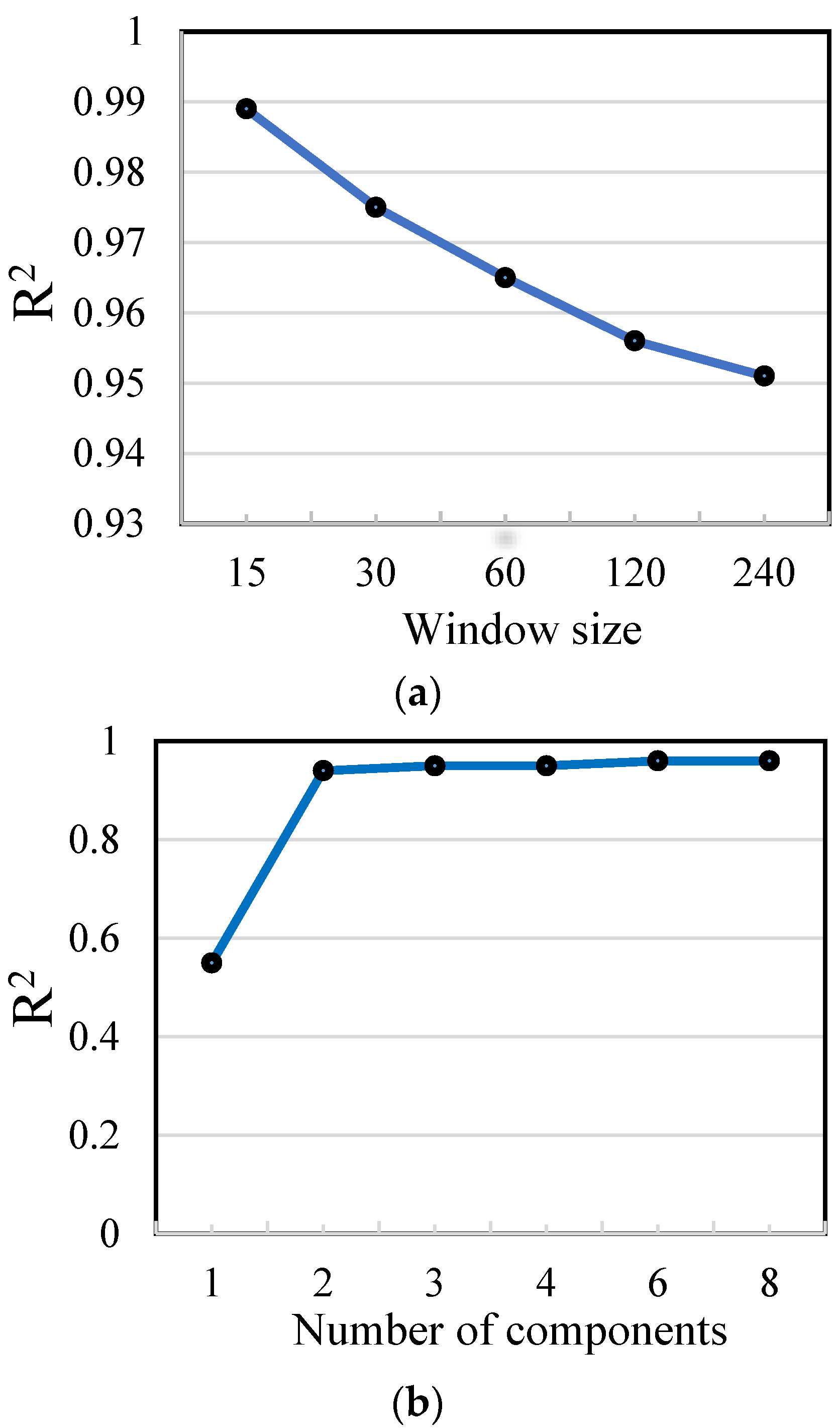
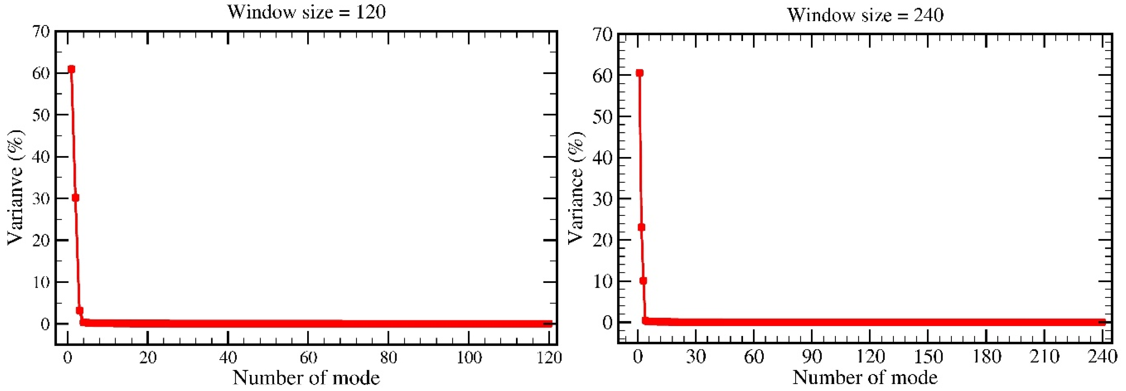
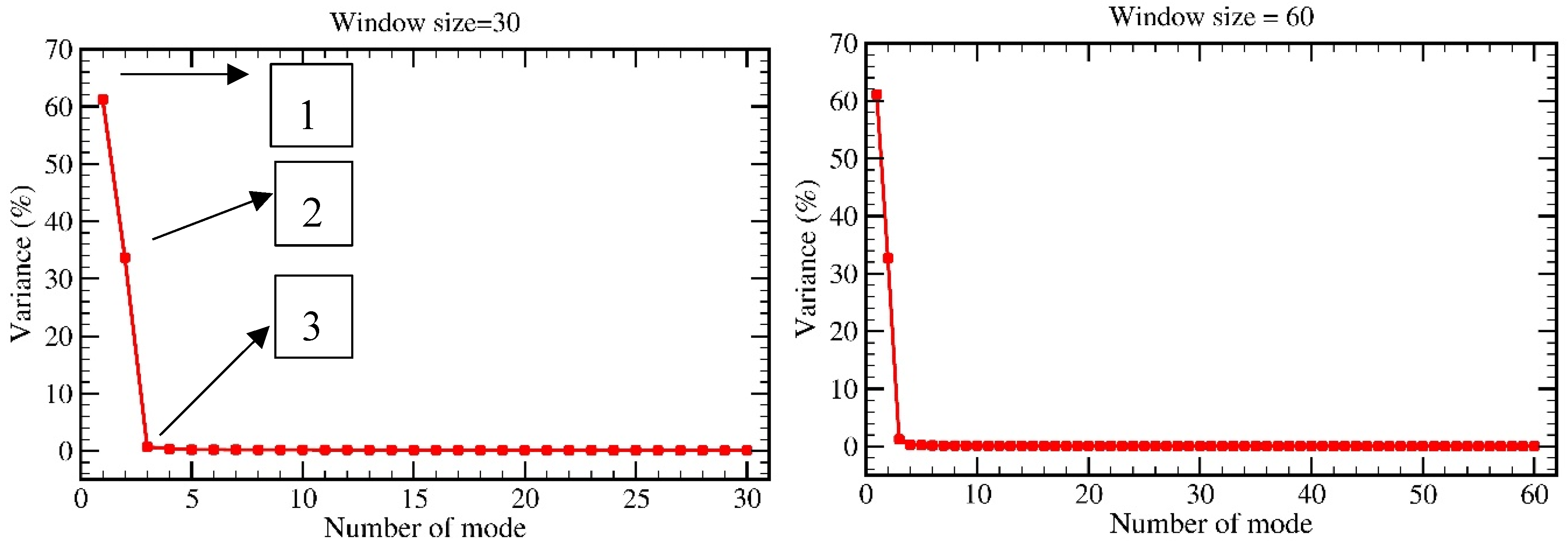
4.2. Determining the Parameters of SSA Algorithm

Determining the window size and number of components are two important parameters in reconstructing a time series by SSA algorithm. Therefore, it is necessary to select the window size and number of components optimally. Figure 6 shows the effects of the number of components in a window size of 60 in reconstructing a time series with 730 images. By increasing the number of components from 1 to 2, the coefficient of determination value (R²) increased significantly between the original data and reconstructed signal by SSA algorithm. Then, by increasing the number of components from two to eight, the R² value was not significantly increased. Figure 6a illustrates the effect of different window sizes on the reconstruction of the same time series with four components. By increasing the window size, the R² value between the original data and reconstructed data was reduced. Using small window sizes to reconstruct a time series with long-distance missing data has no favorable results, and using large window sizes not only reduces the accuracy of reconstruction, it also increases the time of processing. Thus, in the present study, a window size of 60 was used to process the time series. In the following, the accurate determination of the number of significant components and window sizes by SSA algorithm are fully described.

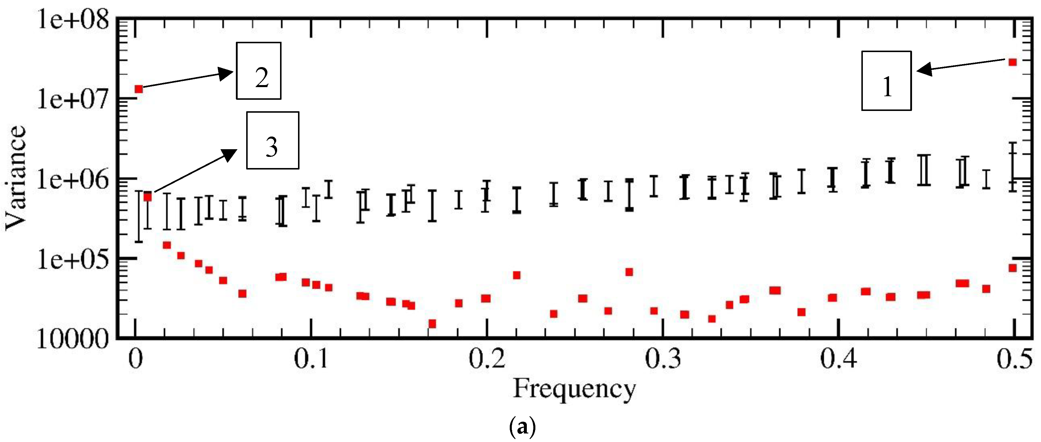
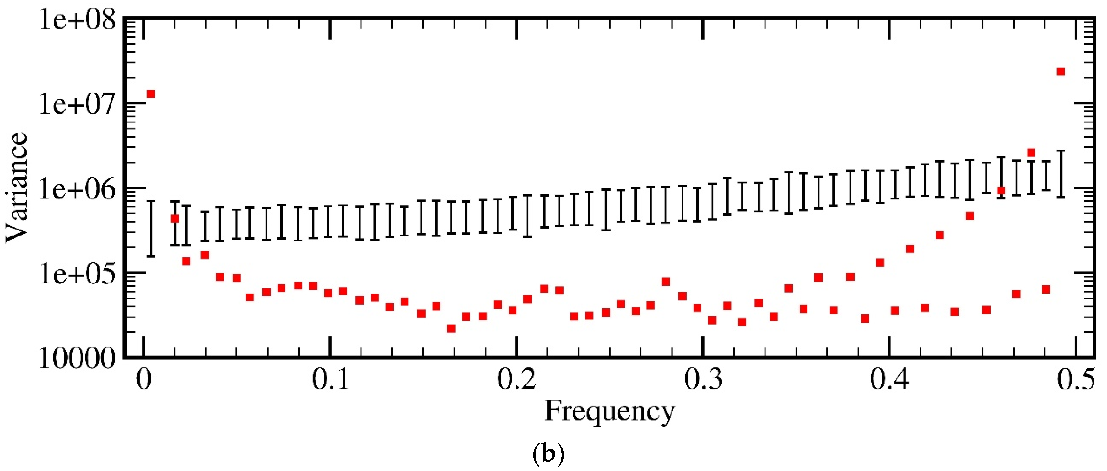
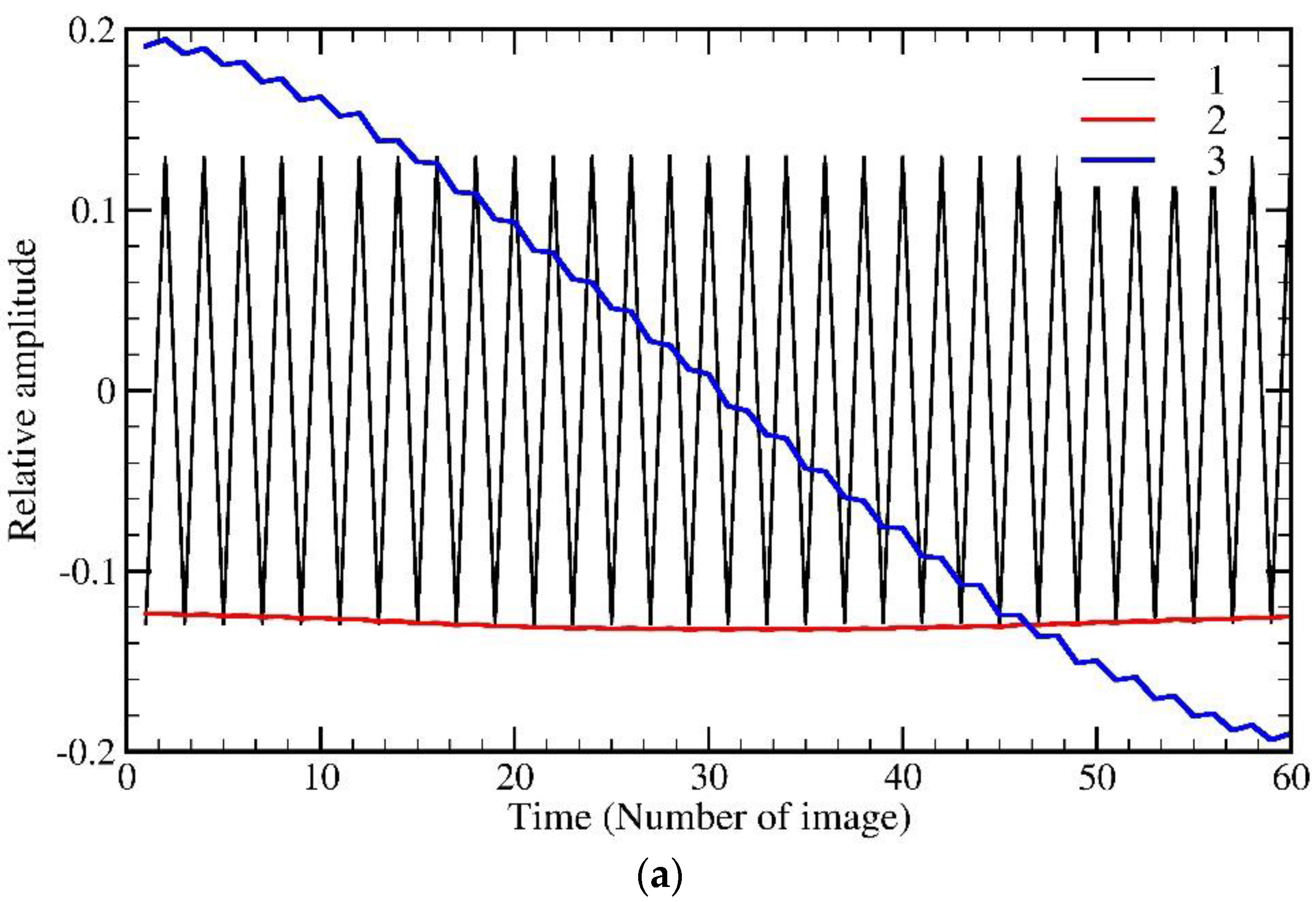
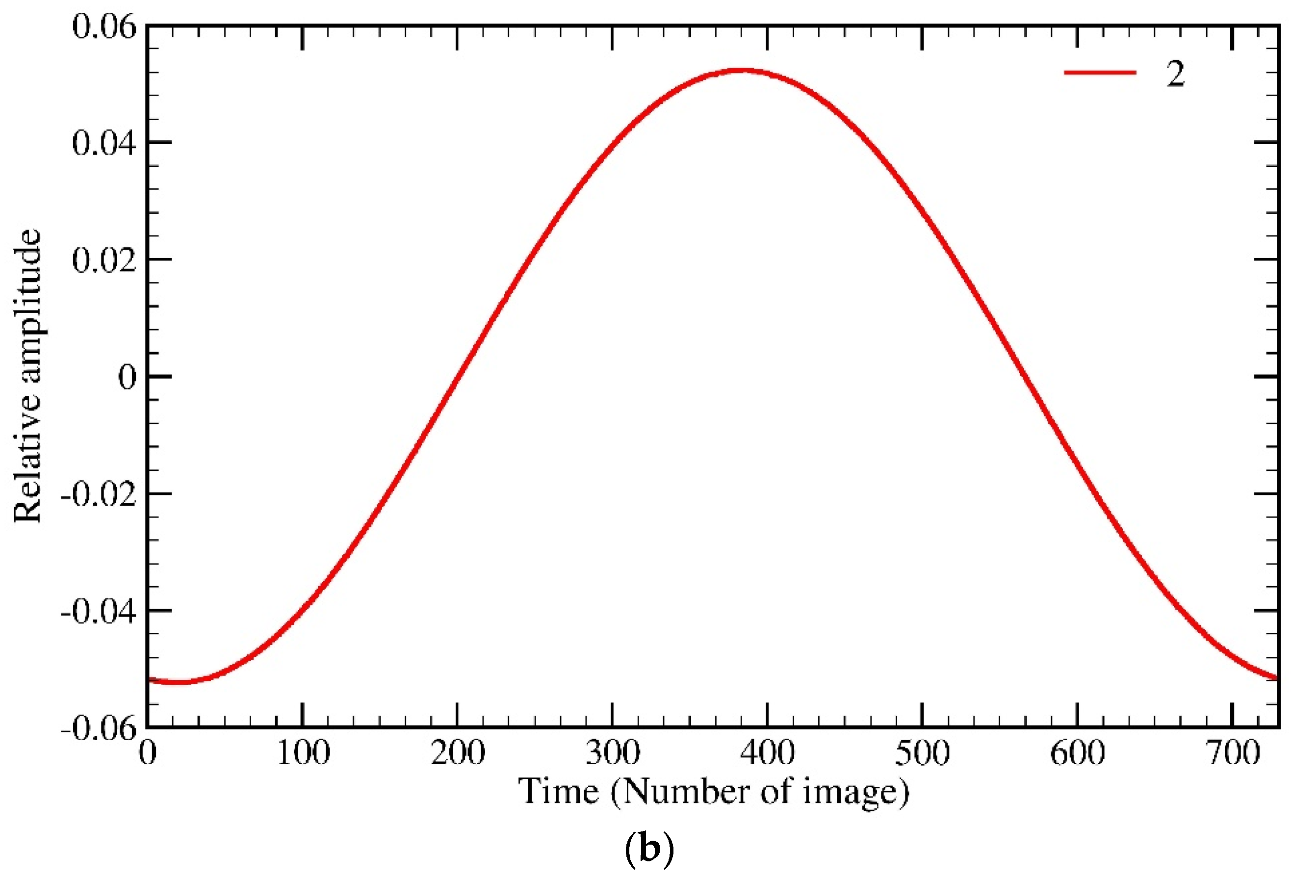
4.3. Determining the Significant Periodic Components in the SSA Algorithm

Figure 7 shows the singular values spectrum of the specific pixel (the one with no missing data) that employs 60 images as the window size. When plotting the singular values of a time series in descending order, we can recognize an initial steep slope that represents signals, and a more or less flat tail related to noise. Since the window size of 60 was selected, SSA divided this time series into 60 components. Therefore, there are 60 modes in the horizontal axis. The vertical axis shows the variance of components. Based on Figure 7, components 1, 2, and 3 have the highest variance, respectively. Since components 1, 2, and 3 are located singly in the figure, each of them shows one trend of changes in the signal [34]. When two components are paired equally, their EOFs are transferred in a quarter-phase (phase difference). These components are effectively indicative of fluctuation in a time series and are a part of periodic components [34].

Figure 8 presents the normalized curve of specific figures in window sizes of 30, 60, 120, and 240. As shown, by selecting the window size of 30 images, components 1 and 2 showed maximum variance in the signal, so that a total of 95% of variance in this time series was related to these components (62% for component 1 and 33% for component 2). By increasing the window size to 60 images, almost the same results were obtained. By increasing the window size to 120 and 240 images, the effect of variance of component 3 increased; as in window size 240, components 1, 2, and 3 have 61%, 24%, and 10% of changes in this time series. In general, this figure showed two important points. Firstly, components 1, 2, and 3 have the highest variance in this time series. On the other hand, the failure to select any of these components to reconstruct this time series causes an inaccurate signal. Secondly, the window size change in this time series will not have a significant effect on the results of signal reconstruction, because by increasing the window size, components 1, 2, and 3 will still have the highest variance.

4.4. Data Basis and Null Hypothesis Basis Monte Carlo Test Results

Figure 9 shows the results of data and null hypothesis EOFs for pure red noise, indicating the power in the data eigenvalues and surrogates data bars versus the frequency associated to EOFs. Obtaining a single frequency for each EOF is not straightforward, given that the EOFs resulting from SSA for an intrinsically periodic time series are not purely sinusoid unless they are composed of entirely strictly periodic components (e.g., synthetic periodic time series). To do so, Allen and Smith (1996) associated a frequency to each EOF by maximizing the R-squared (R²) with a pure sinusoid for better visualization. The top graph of Figure 9 shows the result of the data-based Monte Carlo test.

Figure 8 illustrates the eigenvalues versus their relevant frequencies at window sizes of 30, 60, 120, and 240 images. Figure 9 shows that components 1, 2, and 3 are significantly major components of this time series with a specific percentile of 97.5%. In this figure, the components are named according to the larger variance, respectively. The frequencies of components 1, 2, and 3 are 0.449, 0.002, and 0.006 (cycle/day), which belong to periods of 2 (2/2 = 1 as daily component), ~500 (500/2 ~250, or almost one year), and 166 (166/2 = 88 days or almost three months as a trend) of the images, respectively.

The null hypothesis EOFs test, which is visible as the lower graph of Figure 9, confirms the significance of these pairs. The null hypothesis-based test has the advantage of having a lower probability of selecting a noise component as a signal component, which helps to identify significant signal better, and thus the result is more reliable [44].

Figure 10 presents the temporal EOFs of the significant components in this time series based on the results of the Monte Carlo test. Component 1 of the image in the Monte Carlo test shows the same day/night temperature changes. As shown, the black lines in both images are repeated every day and night. Component 2 of the image indicates the annual temperature changes, and component 3 almost shows the seasonal periods in this time series (components 2 and 3 are shown in red and blue colors in Figure 10a), which belongs to a significant trend. Component 2 is shown as a small part of the annual period, and it is periodically repeated in approximately each of the 730 images. For a better display, component 2 is drawn in window size 730 (Figure 10b). Component 3 is only part of a periodic signal with 166 images, which is shown as a trend in the window size of 60 images (Figure 10a).

Generally, the results of the Monte Carlo test and those of other tests showed that window size 60 yielded reliable results for the reconstruction of this time series. In window size 60, three significant components can be differentiated in this time series. Therefore, three components, including 1, 2, and 3, were used to reconstruct the whole time series in window size 60 in M-SSA.

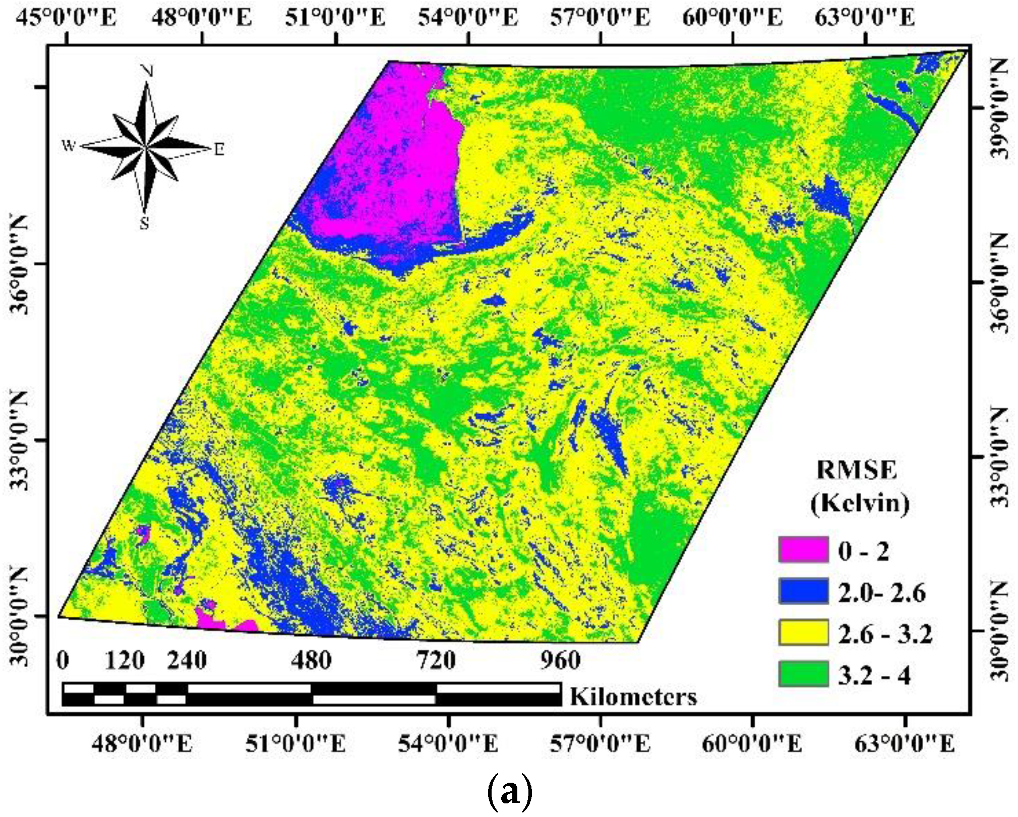
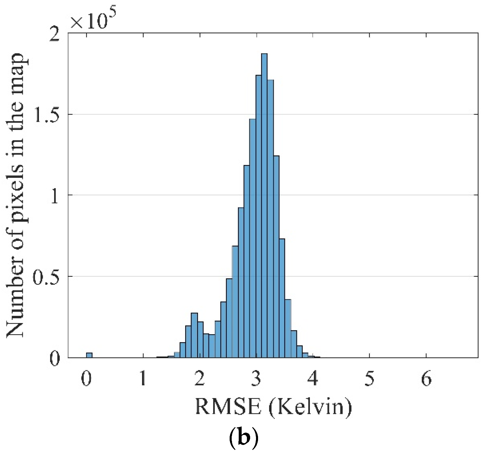
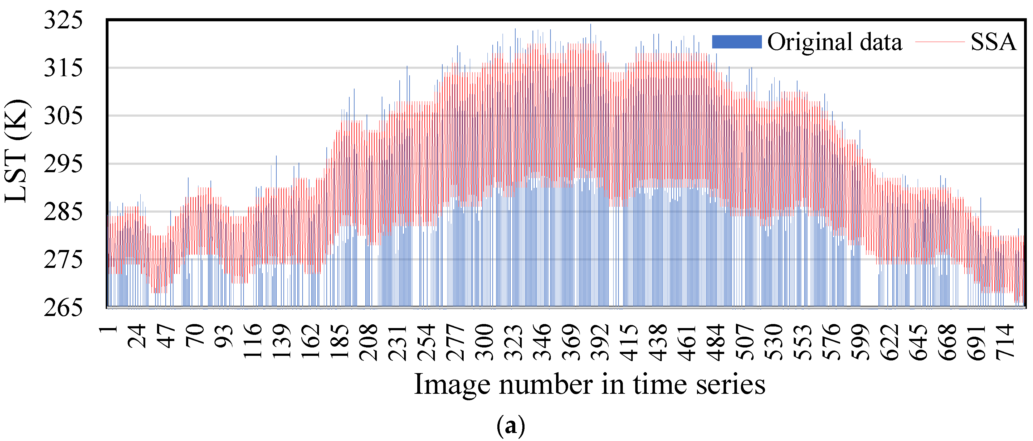
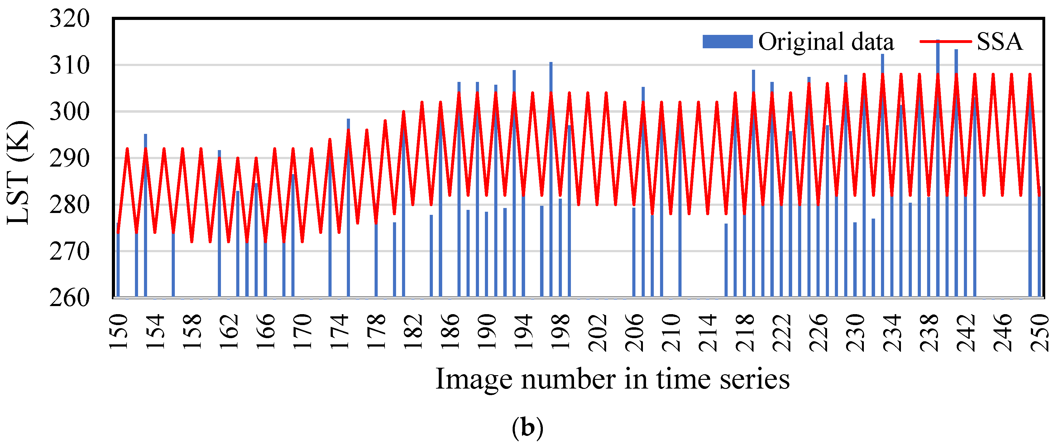
4.5. Assessment of Results

Figure 11 displays the RMSE map between the original data and reconstructed data by SSA along an annual LST time series with 730 images. As shown in Figure 11a, the minimum RMSE is observed on the Caspian Sea. At other points, the RMSE is variable from 2 to 4 kelvin (K). Figure 11b shows the histogram of the RMSE map of LST. Overall, the mean RMSE of the reconstructed LST by SSA algorithm in the studied time series with 730 images is 2.95 K.

Figure 12 indicates image number 215 (18 April 2015) as an example in the studied time series before and after reconstruction by the SSA algorithm. As shown in Figure 12a, 50.25% of the data of this image are missing due to cloud cover (black areas). It should also be noted that in addition to the missing data in this image, the outlier data exist, which are not detectable spatially but are detectable in a time domain. Hence, the missing data cannot be reconstructed by spatial interpolation techniques. According to Figure 12b, the SSA algorithm could reconstruct the missing and outlier data of the LST image by spatio-temporal interpolation technique. The reconstructed LST image shows that the missing data (due to cloud coverage with zero value) of the image that are filled by SSA are similar to the main image pattern, i.e. the spatial pattern after reconstruction is rather smooth locally (no “salt” and “pepper” appearance). This is indicative of the capability of this algorithm in solving the missing and outlier data problem caused by cloud cover.

As an example, Figure 13 indicates a time series along a pixel together with the reconstruction results of the SSA algorithm. As shown, the SSA algorithm effectively reconstructed the missing and outlier data in this time series. According to Figure 13a, the temperature difference between day and night is lower at the start and end of the time series than the middle parts of this time series. The SSA algorithm was effective in the identification of these changes and trends, and considered these temperature changes in the reconstructed signal. As shown in Figure 13a, there is a growing temperature rise from the start to the middle of time series, followed by a decreasing trend. This trend is the same annual temperature changes that are being considered as component 2 in determining the significant periodic components. Partial thermal fluctuations are observed during the year, which are detectable as multi-month periods in Figure 13. These changes are due to considering component 3. Figure 13b presents a more translucent display of a part of a reconstructed signal. The temperature changes during the day and night are seen in this figure, which are caused by component 1. Hence, the failure to consider any of the mentioned components in the reconstruction of this time series causes inaccurate findings.

5. Conclusions

In the present study, the SSA algorithm was used to reconstruct the missing data caused by cloud cover in a daily LST time series of a MODIS sensor during 2015. According to the results of an accuracy evaluation of the SSA algorithm, the mean reconstruction error in the whole studied region was 2.95 °K. These results are promising owing to the amount of missing data caused by cloud cover in the time series with 730 LST images, because these figures are in line with the temperature measurement errors (±3 °K) by remote sensing [46]. The findings showed the minimum reconstruction error on the Caspian Sea (<2.6 °K). This is due to the high thermal specific capacity of water, which results in little and gradual water temperature changes per day and during the year. Hence, the reconstructed signal is more compatible with the original data. Malamiri and Khormizie (2017) reconstructed a daily MODIS LST time series over a year by the HANTS algorithm and reported that the reconstruction error of the LST time series was lower on the sea [47]. Further, the results of Malamiri and Khormizie (2017) showed that the reconstruction error in the annual LST time series during the day from a MODIS sensor in this study region was 3.87 °K on average [47]. Therefore, the reconstruction accuracy is higher in the SSA algorithm than in the HANTS algorithm. This is because only temporal interpolation is used in the HANTS algorithm; whereas, spatio-temporal interpolation is used in the SSA algorithm in M-SSA to reconstruct the time series. Since the daily MODIS LST time series includes LST during the day and night, this time series can be processed in two different ways to reconstruct the effects of cloud cover. First, LST images during the day and at night can be reconstructed into two separate time series. Second, LST images can be put together as a day/night sequence and reconstructed as a time series. In this study, the second method was applied. When a daily MODIS LST time series is used in a day/night sequence, a significant component (component 1, which indicates the day/night sequence) is created. When this component is used to reconstruct the time series, the accuracy will increase dramatically, because the daily missing data caused by cloud cover at certain points may be present during the night and vice versa.

Three significant components were identified in a daily MODIS LST time series with a day/night sequence. The first component was the same day and night temperature changes, the second component was annual temperature changes, and the third component was seasonal temperature changes. The number of significant components (periods or trends) varies in different time series. Reconstructing the hourly LST time series, Malamiri (2015) reported three significant periodic components—24 h, 12 h, and 8 h—were differentiated in the window size of 72 h [19].

According to the findings, the SSA algorithm can effectively resolve the missing data problem in a MODIS LST time series. In research using SSA and M-SSA algorithms, Ghafarian et al. (2012) reconstructed the time series of hourly LST data, and showed an absolute mean error of 2.25 °K in an hourly time series with 63% missing data caused by cloud cover [1]. Another study indicated that M-SSA using spatio-temporal correlation effectively reconstructed the MODIS LAI [38]. In general, the results showed that the SSA algorithm could be effectively used to resolve the missing data problem caused by cloud cover in a daily MODIS LST time series.

References

- Ghafarian, H.R.; Menenti, M.; Jia, L.; den Ouden, H. Reconstruction of cloud-free time series satellite observations of land surface temperature. EARSel eProc. 2012, 11, 123–131. [Google Scholar]
- Xu, Y.; Shen, Y. Reconstruction of the land surface temperature time series using harmonic analysis. Comput. Geosci. 2013, 61, 126–132. [Google Scholar] [CrossRef]
- Sobrino, J.A.; El Kharraz, J.E.; Li, Z.-L. Surface temperature and water vapour retrieval from MODIS data. Int. J. Remote Sens. 2003, 24, 5161–5182. [Google Scholar] [CrossRef]
- Running, S.W.; Justice, C.O.; Salomonson, V.; Hall, D.; Barker, J.; Kaufmann, Y.J.; Strahler, A.H.; Huete, A.R.; Muller, J.P.; Vanderbilt, V.; et al. Terrestrial remote sensing science and algorithms planned for EOS/MODIS. Int. J. Remote Sens. 1994, 15, 3587–3620. [Google Scholar] [CrossRef]
- Wan, Z.; Zhang, Y.; Zhang, Q.; Li, Z.L. Validation of the land-surface temperature products retrieved from Terra Moderate Resolution Imaging Spectroradiometer data. Remote Sens. Environ. 2002, 83, 163–180. [Google Scholar] [CrossRef] [Green Version]
- Sun, D.; Pinker, R.T.; Basara, J.B. Land surface temperature estimation from the next generation of Geostationary Operational Environmental Satellites: GOES M–Q. J. Appl. Meteorol. 2004, 43, 363–372. [Google Scholar] [CrossRef]
- Estes, M.G., Jr.; Al-Hamdan, M.Z.; Crosson, W.; Estes, S.M.; Quattrochi, D.; Kent, S.; McClure, L.A. Use of remotely sensed data to evaluate the relationship between living environment and blood pressure. Environ. Health Perspect. 2009, 117, 1832. [Google Scholar] [CrossRef] [PubMed]
- Tatem, A.J.; Goetz, S.J.; Hay, S.I. Terra and Aqua: New data for epidemiology and public health. Int. J. Appl. Earth Obs. Geoinf. 2004, 6, 33–46. [Google Scholar] [CrossRef] [PubMed]
- Schmugge, T.; French, A.; Ritchie, J.C.; Rango, A.; Pelgrum, H. Temperature and emissivity separation from multispectral thermal infrared observations. Remote Sens. Environ. 2002, 79, 189–198. [Google Scholar] [CrossRef]
- Rousta, I.; Doostkamian, M.; Haghighi, E.; Mirzakhani, B. Statistical-Synoptic Analysis of the Atmosphere Thickness Pattern of Iran’s Pervasive Frosts. Climate 2016, 4, 41. [Google Scholar] [CrossRef]
- Soltani, M.; Laux, P.; Kunstmann, H.; Stan, K.; Sohrabi, M.M.; Molanejad, M.; Sabziparvar, A.A.; SaadatAbadi, A.R.; Ranjbar, F.; Rousta, I.; et al. Assessment of climate variations in temperature and precipitation extreme events over Iran. Theor. Appl. Climatol. 2016, 126, 775–795. [Google Scholar] [CrossRef]
- Soltani, M.; Zawar-Reza, P.; Khoshakhlagh, F.; Rousta, I. Mid-latitude Cyclones Climatology over Caspian Sea Southern Coasts–North of Iran. Available online: https://ams.confex.com/ams/21Applied17SMOI/webprogram/Paper246601.html (accessed on 20 June 2018).
- Rousta, I.; Soltani, M.; Zhou, W.; Cheung, H.H. Analysis of Extreme Precipitation Events over Central Plateau of Iran. Am. J. Clim. Chang. 2016, 5, 297. [Google Scholar] [CrossRef]
- Rousta, I.; Doostkamian, M.; Taherian, A.M.; Haghighi, E.; Ghafarian Malamiri, H.R.; Ólafsson, H. Investigation of the Spatio-Temporal Variations in Atmosphere Thickness Pattern of Iran and the Middle East with Special Focus on Precipitation in Iran. Climate 2017, 5, 82. [Google Scholar] [CrossRef]
- Rousta, I.; Javadizadeh, G.; Dargahian, F.; Ólafsson, H.; Shiri Karimvandi, A.; Vahedinejad, S.H.; Doostkamian, M.; Monroy Vargas, E.R.; Asadolahi, A. Investigation of Vorticity during Prevalent Winter Precipitation in Iran. Adv. Meteorol. 2018, in press. [Google Scholar]
- Julien, Y.; Sobrino, J.A. Comparison of cloud-reconstruction methods for time series of composite NDVI data. Remote Sens. Environ. 2010, 114, 618–625. [Google Scholar] [CrossRef]
- Zhou, J.; Jia, L.; Menenti, M. Reconstruction of global MODIS NDVI time series: Performance of harmonic analysis of time series (HANTS). Remote Sens. Environ 2015, 163, 217–228. [Google Scholar] [CrossRef]
- Ackerman, S.A.; Strabala, K.I.; Menzel, W.P.; Frey, R.A.; Moeller, C.C.; Gumley, L.E. Discriminating clear sky from clouds with MODIS. J. Geophys. Res. Atmos. 1998, 103, 32141–32157. [Google Scholar] [CrossRef] [Green Version]
- Ghafarian Malamiri, H.R. Reconstruction of Gap-Free Time Series Satellite Observations of Land Surface Temperature to Model Spectral Soil Thermal Admittance. Available online: https://repository.tudelft.nl/islandora/object/uuid:63dc3402-9fd6-4594-a00e-7aa5ae2501aa?collection=research (accessed on 20 June 2018).
- Jia, L.; Shang, H.; Hu, G.; Menenti, M. Phenological response of vegetation to upstream river flow in the Heihe Rive basin by time series analysis of MODIS data. Hydrol. Earth Syst. Sci. 2011, 15, 1047–1064. [Google Scholar] [CrossRef] [Green Version]
- Roerink, G.; Menenti, M.; Verhoef, W. Reconstructing cloudfree NDVI composites using Fourier analysis of time series. Int. J. Remote Sens. 2000, 21, 1911–1917. [Google Scholar] [CrossRef]
- Verhoef, W. Application of harmonic analysis of NDVI time series (HANTS). Fourier Anal. Temp. Am. Cont. 1996, 108, 19–24. [Google Scholar]
- Verhoef, W.; Menenti, M.; Azzali, S. Cover A colour composite of NOAA-AVHRR-NDVI based on time series analysis (1981–1992). Int. J. Remote Sens. 1996, 17, 231–235. [Google Scholar] [CrossRef]
- Menenti, M.; Azzali, S.; Verhoef, W.; Van Swol, R. Mapping agroecological zones and time lag in vegetation growth by means of Fourier analysis of time series of NDVI images. Adv. Space Res. 1993, 13, 233–237. [Google Scholar] [CrossRef]
- Jiang, X.; Wang, D.; Tang, L.; Hu, J.; Xi, X. Analysing the vegetation cover variation of China from AVHRR-NDVI data. Int. J. Remote Sens. 2008, 29, 5301–5311. [Google Scholar] [CrossRef]
- Julien, Y.; Sobrino, J.A.; Verhoef, W. Changes in land surface temperatures and NDVI values over Europe between 1982 and 1999. Remote Sens. Environ. 2006, 103, 43–55. [Google Scholar] [CrossRef]
- Alfieri, S.M.; Lorenzi, F.D.; Menenti, M. Mapping air temperature using time series analysis of LST: The SINTESI approach. Nonlinear Proc. Geophys. 2013, 20, 513–527. [Google Scholar] [CrossRef]
- Broomhead, D.S.; King, G.P. Extracting qualitative dynamics from experimental data. Phys. D Nonlinear Phenom. 1986, 20, 217–236. [Google Scholar] [CrossRef]
- Kondrashov, D.; Ghil, M. Spatio-temporal filling of missing points in geophysical data sets. Nonlinear Proc. Geophys. 2006, 13, 151–159. [Google Scholar] [CrossRef] [Green Version]
- Vautard, R.; Yiou, P.; Ghil, M. Singular-spectrum analysis: A toolkit for short, noisy chaotic signals. Phys. D Nonlinear Phenom. 1992, 58, 95–126. [Google Scholar] [CrossRef]
- Golyandina, N.; Zhigljavsky, A. Singular Spectrum Analysis for Time Series; Springer Science & Business Media: Berlin, Germany, 2013; Available online: https://books.google.com.hk/books?hl=zh-TW&lr=&id=CUpEAAAAQBAJ&oi=fnd&pg=PP5&dq=Singular+Spectrum+Analysis+for+time+series.+&ots=zF6W4hag3S&sig=yuKb4t8umEUW2AQXkcGD28nfZC8&redir_esc=y#v=onepage&q=Singular%20Spectrum%20Analysis%20for%20time%20series.&f=false (accessed on 20 June 2018).
- Golyandina, N.; Nekrutkin, V.; Zhigljavsky, A.A. Analysis of Time Series Structure: SSA and Related Techniques; Chapman and Hall/CRC: Washington, DC, USA, 2001. [Google Scholar]
- Ghil, M.; Vautard, R. Interdecadal oscillations and the warming trend in global temperature time series. Nature 1991, 350, 324. [Google Scholar] [CrossRef]
- Vautard, R.; Ghil, M. Singular spectrum analysis in nonlinear dynamics, with applications to paleoclimatic time series. Phys. D Nonlinear Phenom. 1989, 35, 395–424. [Google Scholar] [CrossRef]
- Yiou, P.; Baert, E.; Loutre, M.F. Spectral analysis of climate data. Surv. Geophys. 1996, 17, 619–663. [Google Scholar] [CrossRef]
- Yiou, P.; Sornette, D.; Ghil, M. Data-adaptive wavelets and multi-scale singular-spectrum analysis. Phys. D Nonlinear Phenom. 2000, 142, 254–290. [Google Scholar] [CrossRef] [Green Version]
- Kondrashov, D.; Shprits, Y.; Ghil, M. Gap filling of solar wind data by singular spectrum analysis. Geophys. Res. Lett. 2010, 37, L15101. [Google Scholar] [CrossRef]
- Wang, D.; Liang, S. Singular Spectrum Analysis for Filling Gaps and Reducing Uncertainties of MODIS Land Products. 2008. Available online: https://ieeexplore.ieee.org/abstract/document/4780153/ (accessed on 20 June 2018).
- Marques, C.A.F.; Ferreira, J.A.; Rocha, A.; Castanheira, J.M.; Melo-Gonçalves, P.; Vaz, N.; Dias, J.M. Singular spectrum analysis and forecasting of hydrological time series. Phys. Chem. Earth 2006, 31, 1172–1179. [Google Scholar] [CrossRef]
- Wan, Z. MODIS Land-Surface Temperature Algorithm Theoretical Basis Document (LST ATBD). Available online: https://modis.gsfc.nasa.gov/data/atbd/atbd_mod11.pdf (accessed on 20 June 2018).
- Wan, Z. New refinements and validation of the collection-6 MODIS land-surface temperature/emissivity product. Remote Sens. Environ. 2014, 140, 36–45. [Google Scholar] [CrossRef]
- Musial, J.P.; Verstraete, M.M.; Gobron, N. Comparing the effectiveness of recent algorithms to fill and smooth incomplete and noisy time series. Atmos. Chem. Phys. 2011, 11, 7905–7923. [Google Scholar] [CrossRef] [Green Version]
- Elsner, J.B.; Tsonis, A.A. Singular Spectrum Analysis: A New Tool in Time Series Analysis; Springer Science & Business Media: New York, NY, USA, 1996. [Google Scholar]
- Allen, M.R.; Smith, L.A. Monte Carlo SSA: Detecting irregular oscillations in the presence of colored noise. J. Clim. 1996, 9, 3373–3404. [Google Scholar] [CrossRef]
- Schoellhamer, D.H. Singular spectrum analysis for time series with missing data. Geophys. Res. Lett. 2001, 28, 3187–3190. [Google Scholar] [CrossRef] [Green Version]
- Li, Z.L.; Tang, B.H.; Wu, H.; Ren, H.; Yan, G.; Wan, Z.; Trigo, I.F.; Sobrino, J.A. Satellite-derived land surface temperature: Current status and perspectives. Remote Sens. Environ. 2013, 131, 14–37. [Google Scholar] [CrossRef] [Green Version]
- Ghafarian Malamiri, H.R.; Khormizie, H.Z. Reconstruction of cloud-free time series satellite observations of land surface temperature (LST) using harmonic analysis of time series algorithm (HANTS). J. RS GIS Nat. Resour. 2017, 8, 37–55. [Google Scholar]
© 2018 by the authors. Licensee MDPI, Basel, Switzerland. This article is an open access article distributed under the terms and conditions of the Creative Commons Attribution (CC BY) license (http://creativecommons.org/licenses/by/4.0/).
Share and Cite
Ghafarian Malamiri, H.R.; Rousta, I.; Olafsson, H.; Zare, H.; Zhang, H. Gap-Filling of MODIS Time Series Land Surface Temperature (LST) Products Using Singular Spectrum Analysis (SSA). Atmosphere 2018, 9, 334. https://doi.org/10.3390/atmos9090334
Ghafarian Malamiri HR, Rousta I, Olafsson H, Zare H, Zhang H. Gap-Filling of MODIS Time Series Land Surface Temperature (LST) Products Using Singular Spectrum Analysis (SSA). Atmosphere. 2018; 9(9):334. https://doi.org/10.3390/atmos9090334
Chicago/Turabian StyleGhafarian Malamiri, Hamid Reza, Iman Rousta, Haraldur Olafsson, Hadi Zare, and Hao Zhang. 2018. "Gap-Filling of MODIS Time Series Land Surface Temperature (LST) Products Using Singular Spectrum Analysis (SSA)" Atmosphere 9, no. 9: 334. https://doi.org/10.3390/atmos9090334