Article

Surface and Tropospheric Water Vapor Variability and Decadal Trends at Two Supersites of CO-PDD (Cézeaux and Puy de Dôme) in Central France

1
Laboratoire de Météorologie Physique, UMR 6016, CNRS, Clermont Auvergne University, 63178 Aubière, France
2
Observatoire de Physique du globe de Clermont-Ferrand, UMS833, CNRS, Clermont Auvergne University, 63178 Aubière, France
3
Lab-STICC/PRASYS, UMR CNRS 6285, ENSTA Bretagne, 29806 Brest, France
4
Laboratoire des Sciences du Climat et de l’Environnement, UMR 8212, CEA, CNRS, Versailles Saint Quentin University, 91198 Gif-sur-Yvette, France
5
Laboratoire de l’Atmosphère et des Cyclones, UMR8105, CNRS, Météo-France, Reunion University, 97715 Saint--Denis, Réunion island, France
*
Author to whom correspondence should be addressed.
Atmosphere 2018, 9(8), 302; https://doi.org/10.3390/atmos9080302
Submission received: 28 May 2018 / Revised: 25 July 2018 / Accepted: 26 July 2018 / Published: 1 August 2018
(This article belongs to the Section Meteorology)

Abstract

:
We present an analysis of decadal in situ and remote sensing observations of water vapor over the Cézeaux and puy de Dôme, located in central France (45° N, 3° E), in order to document the variability, cycles and trends of surface and tropospheric water vapor at different time scales and the geophysical processes responsible for the water vapor distributions. We use meteorological stations, GPS (Global Positioning System), and lidar datasets, supplemented with three remote sources of water vapor (COSMIC-radio-occultation, ERA-interim-ECMWF numerical model, and AIRS-satellite). The annual cycle of water vapor is clearly established for the two sites of different altitudes and for all types of measurement. Cezeaux and puy de Dôme present almost no diurnal cycle, suggesting that the variability of surface water vapor at this site is more influenced by a sporadic meteorological system than by regular diurnal variations. The lidar dataset shows a greater monthly variability of the vertical distribution than the COSMIC and AIRS satellite products. The Cézeaux site presents a positive trend for the GPS water vapor total column (0.42 ± 0.45 g·kg−1/decade during 2006–2017) and a significant negative trend for the surface water vapor mixing ratio (−0.16 ± 0.09 mm/decade during 2002–2017). The multi-linear regression analysis shows that continental forcings (East Atlantic Pattern and East Atlantic-West Russia Pattern) have a greater influence than oceanic forcing (North Atlantic Oscillation) on the water vapor variations.

1. Introduction

Water under its three phases is a key element of the atmosphere. Atmospheric icing occurs in high altitude clouds, like cirrus, which have been recognized as important regulators of the radiative balance of the earth’s atmosphere system [1], and at the top of convective clouds with important issues for aircraft security [2]. Under the liquid phase, clouds and precipitation are important components in the Earth’s energy budget and water cycle, the Earth’s climate, and climate variability [3]. Water vapor is the main contributor to the greenhouse effect [3]. In the lower troposphere, water vapor acts as a resource for precipitation, providing latent heating and diabatic heating to weather systems [4]. In the free troposphere, anomalously dry layers can be interpreted as small-scale features of stratospheric intrusions [5,6]. For these reasons, water vapor is an Essential Climate Variable (ECV) of the Global Climate Observing System (GCOS) program [7].
Wulfmeyer et al. [8] presented recently a review of the water and energy cycles, highlighting two scientific questions essential for the environment and society. They deal with the predictability of extreme events and with the natural and anthropogenic causes of the change of regional and global water and energy cycles. Dedicated centers, such as the European Center for Medium-Range Weather Forecasting (ECMWF), collect and provide data for climate studies, weather forecasting or other purposes. Recently, Noh et al. compared water vapor retrievals including the ERA-Interim reanalyze to radiosondes and highlighted some positive mean biases for relative humidity, especially over the upper troposphere [9].
To develop and maintain long term atmospheric observation supersites is then important for climate issues, comparisons with global model outputs, and satellite validation. CO-PDD (Cézeaux-Opme-puy de Dôme) is an instrumented site for atmospheric research located near Clermont-Ferrand (45° N, 3° E), labeled nationally and involved in international programs and networks such as GAW (Global Atmospheric Watch) or ACTRIS-2 (Aerosol Cloud and Trace Gases Research Infrastructure). It produces in situ and remote sensing measurements of atmospheric components including water vapor, clouds, and precipitations [10]. The objective of CO-PDD is to document the evolution of the composition of the troposphere by proposing to the scientific community a structure for the reception of experiments and a set of long-term measurements to document the processes linking gases, aerosols, cloud condensation and ice nuclei, clouds, and precipitation. Water vapor plays a central role linking many of these atmospheric processes. For example, Zhao et al. recently explored the role of the water vapor content below the freezing level in the response of storm electrical processes to increased concentrations of cloud condensation nuclei [11]. The objective of this paper is then to analyze decadal observations of water vapor over Cezeaux and puy de Dôme, two sites of CO-PDD, in order to document the variability and cycles of water vapor at different time scales and the geophysical processes responsible for the water vapor distributions using a multi instrumental approach.
In this paper, Section 2 provides a description of all data sets used in the study. Section 3 presents the methodology and the numerical tools. Section 4 presents the seasonal cycle and short time variability of water vapor. Section 5 provides the estimation of the contributions of geophysical forcings. Section 6 describes the long term behavior of water vapor and Section 7 summarizes the paper.

2. Data Sets

In this Section we present the instrumented site, instrumentation and in-situ, remote sensing, and satellite data used in this study.

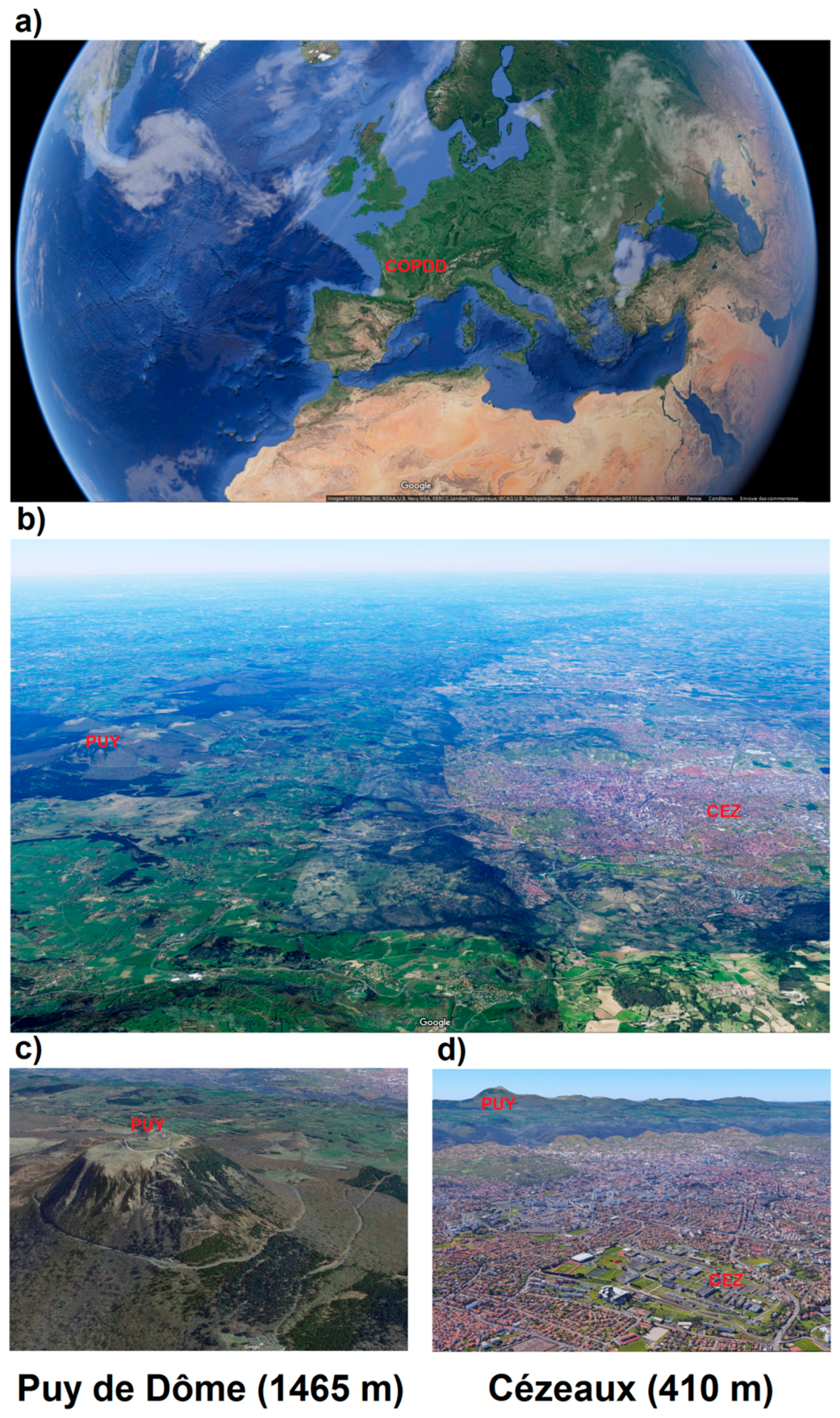
2.1. CO-PDD, the Cézeaux, Opme, and Puy de Dôme Sites

2.1.1. Scientific Context, Networks, and Geographical Location

The puy de Dôme has a very long history related to atmospheric observation, beginning in 1876 when the first French meteorological mountain observatory was open. CO-PDD is now an atmospheric measurement site made up of the puy de Dôme microphysical and chemical station (1465 m, 45.77° N, 2.96° E), located away from immediate sources of pollution, of the Opme rain measurement site (680 m, 45.71° N, 3.09° E), located in a rural area and of the remote sensing Cézeaux University site (410 m, 45.76° N, 3.11° E), located in peri-urban area, near the town of Clermont-Ferrand. A situation map is provided in Figure 1. Puy de Dôme is now a global GAW station and CO-PDD is involved in the ACTRIS-2 and ICOS European infrastructures and its French components ACTRIS-FR and ICOS-FR [10,12]. The research based on CO-PDD data aims to document the evolution of the composition of the troposphere, by improving our knowledge on:
  • The temporal variations of the properties of the gases, aerosols, and clouds on the medium and long-term and their vertical distribution in the troposphere.
  • The processes linking these different atmospheric components (gas, aerosol, cloud).
  • The impact of anthropogenic changes on the composition of the troposphere, and their consequences in terms of climate (cloud, radiation) and meteorology (precipitation).
A summary of the data sets used in this study is provided in Table 1.

2.1.2. Meteorological Stations

Near ground humidity measurements are available at Cézeaux since 2002 and at puy de Dôme since 1995. The meteorological sensors of the Cézeaux and puy de Dôme sites are Vaisala HMP45 (HUMICAP 180 humidity sensor and Pt100 temperature sensor). The accuracy of the humidity sensor is ±2% for a temperature equal to 20 °C and relative humidity values between 0% and 90%; and ±3% for relative humidity values above 90%. The temperature dependence of the humidity sensor is ±0.05% per °C. The temperature sensor has an accuracy of ±0.2 °C at 20 °C [13]. The water vapor mixing ratios (WVMR) are calculated from relative humidity, pressure, and temperature using the Hyland–Wexler formula for the calculation of saturated water vapor pressure [14].

2.1.3. Spectrometer

A CRDS (Cavity Ring Down Spectrometer) commercialized by Picarro is in operation at the puy de Dôme station since April 2011. Over this period three instruments have been used. The first one (G1301 model) was measuring CO2, CH4, and H2O from April 2011 to February 2015, whereas the next two (G2401 model) were measuring in addition CO respectively from February 2015 to August 2016, and from August 2016 up to now. Wavelength-Scanned Cavity Ring Down Spectroscopy is a time-based measurement using a near-infrared laser to quantify spectral features of molecules in a gas circulating in an optical measurement cavity [15]. The effective path length of up to 20 km optimizes precision and sensitivity. The measurement time interval of H2O is about 5 s, and in this work we used hourly means. The precision provided by the manufacturer is 50 ppm. Unlike CO2 and CH4, there is no regular calibration for water vapor. The raw data are corrected according to a calibration against a calibrated hygrometer [16,17], which is applied to all CRDS-Picarro analyzers:
  H c a l = 0.772 ×   H r a w + 0.019493   × H r a w 2  
The scatterplot comparing direct coincidences between meteorological station and Picarro CRDS WVMR at the puy de Dôme station (not shown) presents a good agreement between the two instruments (R² = 0.98, regression line equation y = 1.0394 × −0.0033).

2.1.4. GPS Ground Receivers

Two ground GNSS (Global Navigation Satellite System) receivers operate continuously on CO-PDD sites since 2006 (CLFD, Cézeaux) and 2013 (PDOM, puy de Dôme). These stations are operated by OPGC/LaMP and data are distributed through the French Permanent Network [18], in the framework of ACTRIS-2 project, observations from these two receivers are continuously analyzed (with around 50 other French ground GNSS receivers) using a dedicated processing in order to retrieve the integrated water vapor (IWV) contents. GPS data were processed using Gipsy/oasis II software version 6.4 in Precise Point Positioning mode [19] using JPL ephemerides and clocks. We apply the IERS2010 recommendations for solid Earth tides model [20] and FES2004 model for the ocean tide loading effect [21]. No atmospheric loading correction is applied. Absolute antenna models are used for transmitters (satellites) and receivers. Second order ionosphere correction is used. Phase ambiguities are fixed using the wide lane phase biases computed by JPL (Jet Propulsion Laboratory) [22]. Tropospheric delays are modeled by time varying Zenith Hydrostatic Delays (ZHDs), Zenith Wet Delays (ZWDs), and horizontal gradients along with their respective Vienna mapping functions [23]. The a priori values for the zenith delays and the values for the mapping functions are computed from 6-hourly ECMWF (European Centre for Medium Range Weather Forecasting) analyses. The ZWD parameters and horizontal gradients are modeled as random walk processes with a 5 min time resolution and corrections to the a priori values is estimated during the data processing. The random walk parameters are fixed to 5 mm/ h and 0.5 mm/ h for the ZWDs and gradients, respectively, following the tests made in previous studies [24,25]. ZWD are converted in IWV using a priori ZHD, Bevis formula [26] and Tm provided by TU-Wien. The precision is about 0.5 mm to 2.5 mm, in agreement with the literature [25].

2.1.5. Raman Lidar

A Raman Lidar is in operation at Cézeaux and produce vertical profiles of water vapor since 2009. It uses a Nd: Yag Quantel laser to emit nominal 60 mJ/pulse at 355 nm, with a repetition rate of 10 Hz. A Galilean telescope expands ten times the beam diameter (50 mm), and reduces the divergence of the laser beam to 0.14 mrad. The reception part is based on:
  • a 400 mm Cassegrain telescope, equipped with a field stops set from 1 mm to 4 mm,
  • a detection box dedicated to the splitting of the collected photons with respect to their wavelength
  • LICEL photomultiplier modules equipped with R7400 Hamamatsu PMT tubes for each different channel.
Water vapor concentrations are calculated using the ratio between 408 nm and 387 nm Raman signals. The calibration coefficient is routinely calculated using ECMWF ERA-Interim specific humidity profiles of the closest grid point to the lidar (45.75° N, 3.125° E). The vertical raw resolution of water vapor profiles is 7.5 m and their typical range is 1–10 km, for a 8 h night session. The acquisition software is based on the principles of automation programming, and on a user-friendly user-machine interface. The system is implemented with a complementary module for the automatic operation management [27]. The water vapor channel has been implemented in 2009, and data from 2010 to 2016 are analyzed in this work. In 2018, a renovation project funded by CNRS-INSU, ACTRIS-FR, and CNES allows to change the aging Quantel laser source for a Spectra Physics Indy Laser with a nominal 100 mJ/pulse, to optimize the infrastructure of the lidar, inside the building of the University, in order to facilitate alignment and quality check operations, to improve the stability of the system, and to add acquisition channels at 532 and 1064 nm wavelengths for aerosol-cirrus measurements (color ratio).

2.2. Satellite Observations

2.2.1. AIRS/AQUA

The Atmospheric Infra-Red Sounder (AIRS) is a cross-track nadir scanning sounder launched on 4 May 2002 on board the Earth Observing System (EOS) of the NASA’s AQUA satellite. AQUA has a near-polar and sun-synchronous orbit of 98.2° inclination and 98.8 min period, at an altitude of 705 km [28]. The repeat cycle period is 233 orbits (16 days) with a ground track repeatability of ±20 km. The equatorial crossing local times are 1:30 a.m. in a descending orbit and 1:30 p.m. in an ascending orbit. Nadir scanning AQUA orbit and AIRS scanning geometry allows sounding most of the globe twice daily. The water vapor profiles are obtained over footprints of 45 km × 45 km, with a vertical resolution of 1 km in the troposphere. The infrared spectrum is measured in 2378 channels covering the spectral range from 3.7 μm to 15.4 μm, 41 of which are being used for water vapor retrieval. The version 6 (6.0.7.0) Level-2 retrieval products created using AIRS IR-Only has been used on the period 31 August 2002–31 August 2017 (AIRS2RET). The spatial resolution is 50 km per 50 km. The water vapor mixing ratios provided on the 9 pressure levels from 925 hPa down to 200 hPa have been used (H2OMMRLEVSTD). Data in a radius of 100 km around the Cézeaux site have been selected. According to the AIRS Version 6 Release Level 2 Product User Guide [29], AIRS is insensitive to water vapor at mixing ratios of less than 15–20 ppm. Moisture profiles are obtained at an accuracy of 15% per 2 km thick layer in the lower troposphere and 20–60% in the upper troposphere.

2.2.2. COSMIC/FORMOSAT

The global positioning system radio occultation method is a relatively new technique based on signal phase delays recorded on a space-qualified GPS-GNSS receiver mounted on low-earth-orbiting satellites [30]. Since April 2006, the COSMIC (Constellation Observing System for Meteorology, Ionosphere, and Climate)/FORMOSAT 3 mission provides radio occultation measurements of vertical profiles of refractivity used to derive vertical profiles of atmospheric temperature and water vapor pressure [31]. We calculated the WVMR profiles using atmospheric and water vapor pressures. We extracted all points from 100 km around the CO-PDD sites using the CDAAC Data Download Interface. Since its launch, data of the COSMIC/FORMOSAT mission have been used in weather and climate studies, including, for example, African weather [32], boundary layer height [33], width of the tropical belt [34], or tropopause inversion layer [35].

3. Methodology and Numerical Tools

3.1. ECMWF ERA-Interim

ERA interim is a reanalysis dataset produced by ECMWF. It covers the period 1979 to now and atmospheric parameters can be extracted at 6-h intervals (00, 06, 12 and 18UT) for latitude–longitude grids from 3° × 3° to 0.125° × 0.125° for 15 isentropic levels and 37 pressure levels between 1 and 1000 hPa. ERA-Interim has replaced the ERA-40 archive. The main advances in the ERA-Interim data assimilation compared to ERA-40 are the 12 h 4D variational analysis (4D-Var), the T255 horizontal original resolution, improvement in the humidity analysis, model physics and data quality control, variational bias correction of satellite radiance data, and other improvements in bias handling [36]. These data sets are currently available in the website of ECMWF [37]. In this study, specific humidity (converted to WVMR) and integrated water content have been extracted for the grid point 45.75° N–3.125° E) in order to compare with observations presented in Section 2.

3.2. Long Term Trend Estimation

Water vapor presents a strong annual cycle. For the best determination of long term trends of water vapor it is necessary to remove the annual cycle before establishing the best fit of a linear trend. This approach is based on the regression analysis, developed by Mastenbrook et al. [38] and applied to detect stratospheric water vapor trends. It consists of fitting equations of the form:
Y ( t ) = a 0 + a 1 · t + a 2 cos ( 2 · π · t I ) + a 3 · sin ( 2 · π · t I ) +   ε ( t )    
This equation is established for each vertical level independently by the least square method. Daily means have been used to calculate the trend. Thus, t is time, a 0 + a 1 t is the equation of the linear trend with a 1 the slope and a 0 the ordinate at the origin, a 2 cos ( 2 · π · t I ) + a 3 sin ( 2 · π · t I ) is the annual cycle during the period of our study, I is the number of data that constitutes annual cycle and ε (t) is the residual term.
This technique reduces the noise related to the maximum and the minimum humidity at certain periods of the year, and then the uncertainty associated with the trend calculation. The meteorological station series at puy de Dôme are a specific case because of the change of location and station instrument in 2010. Then the trend of this data set will be estimated by separating two periods, 1995–2010 and 2011–2017.
The uncertainty of the trend is related to the statistical error of the slope, which represents the geophysical variability of the humidity data. We are in the framework of the Student law, which allows the estimation of the statistical error on the slope of the regression line by:
Δ a 1 = σ ^ a 1 · t ( 1 ) / 2 n 2
with:
σ ^ a 1 = σ ^ ε n · V ( x )   and   σ ^ ε = 1 n 2 · t = 1 n ε ( t ) 2
where n is the number of measurements x with a sampling of one day, V ( x )   is the variance of the observation variable and t ( 1 ) / 2 n 2 is the quantile of the Student’s t distribution, equal to 1.645 at 95% level of confidence.

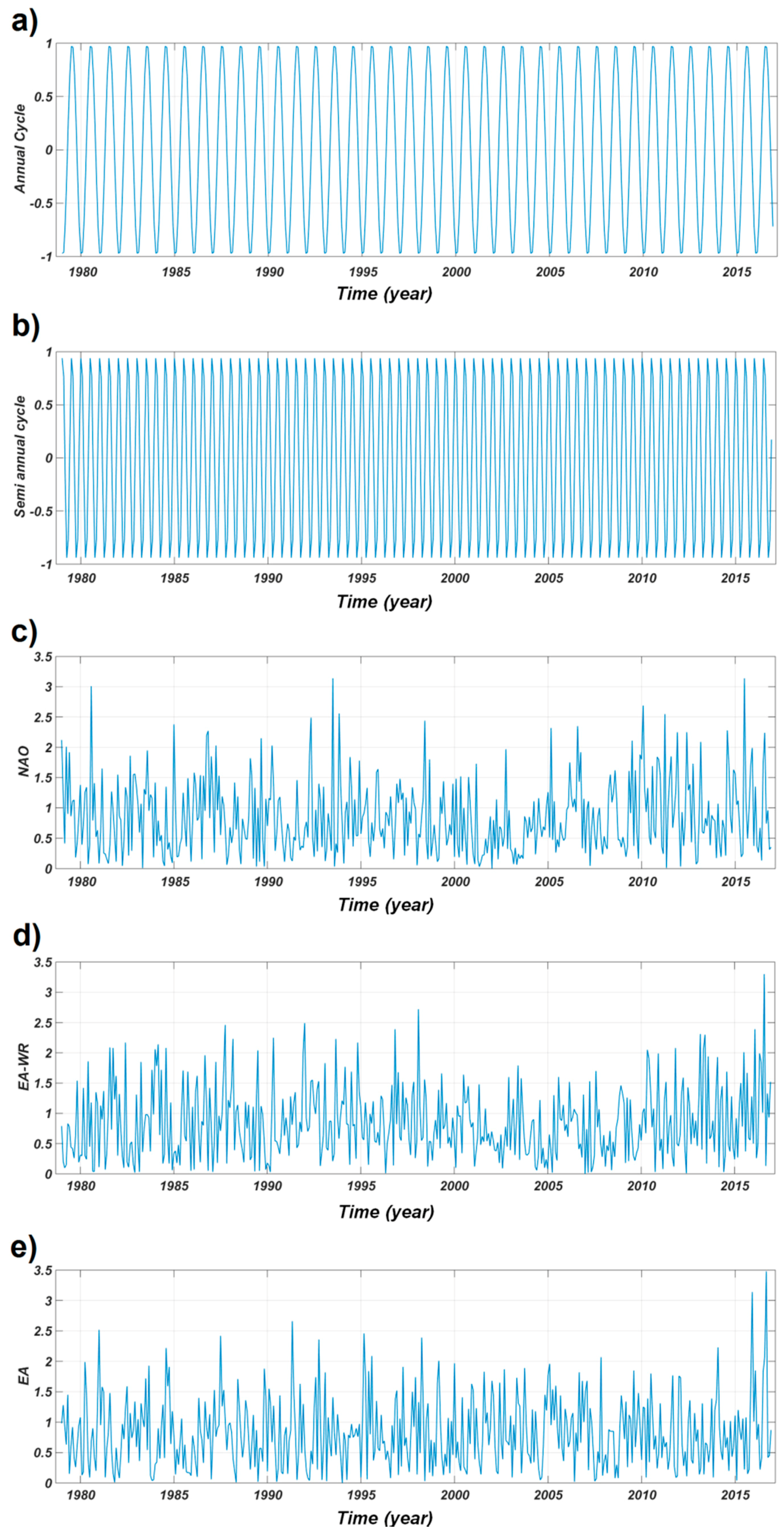
3.3. Determination of the Influence of Geophysical Forcings on Water Vapor Variations

We aim to estimate the influence of geophysical forcings on water vapor distributions. We must first determine that geophysical forcings can potentially influence the water vapor. For that we used the monthly teleconnection indexes calculated from NCEP/NCAR reanalysis data and published by NOAA [39].
The teleconnection indexes of 10 geophysical forcings are published, but some of them concern regions far from Clermont-Ferrand. Finally, we only used three teleconnection indexes:
  • North Atlantic Oscillation (NAO).
  • East Atlantic Pattern (EA).
  • East Atlantic-West Russia Pattern (EA-WR).
Discovered in the 1920s, NAO is a large scale meridian dipole anomaly in sea-level pressure, with the two centers of action located approximately over Iceland and the Azores [40]. It has been shown that NAO has a strong influence on European regional distributions of surface temperature [41], precipitations [42], and ground level aerosols [43].
EA was first described by Wallace and Gutzler [44] as an anomalously high 500 mb height anomaly over the subtropical North Atlantic and Eastern Europe when in positive mode. It is a second mode of inter-annual variability of the tropospheric circulation in that area. Particularly in Southern Europe, the EA pattern is at least as important as the NAO for explaining inter-annual variations of sensible climate variables such as air temperatures, sea-surface temperatures, precipitation, and wind [45].
EA-WR is one of the three prominent teleconnection patterns that affect Eurasia throughout year. This pattern has been referred to as the Eurasia-2 pattern by Barnston and Livezey [46]. It is a zonally oriented pattern with four main anomaly centers, located over Western Europe, Caspian Sea, Northern China, and central North Atlantic. Over the eastern Mediterranean region, the positive EAWR winter periods are associated with more intense northern air flows [47]. EA-WR has a strong impact on the coupling between the sub-tropical Atlantic Jet and the African Jet, which in turn affects the climate variability over Europe from mid-winter to late spring [48].
In addition, the tropospheric water vapor presents annual and semiannual cycles, parameterized on a monthly basis as follows:
  Y annual   ( t ) = cos ( 2 · π · t 12 + φ )  
and:
  Y semiannual   ( t ) = cos ( 2 · π · t 6 + φ )  
where φ = 2 · π · θ 180 .
With θ being the phase coefficient between the water vapor signal and the annual or semi-annual sinusoidal functions, determined by maximizing the correlation between the variation of water vapor and the sinusoidal functions. The time evolution of the teleconnection indexes used and of the annual and semiannual cycles is represented in Figure 2.
Finally, the method of estimation of the influence of the geophysical forcings on water vapor is based on a multiple regression fitting, the observed variable being decomposed as the sum of the contributions of all forcings, annual and semiannual cycles, and a residual term ε minimized by least-squares approach:
  Y ( t ) = β 0 + β 1 · t + β 2 · Y semiannual   ( t ) + β 3 · Y annual ( t ) + β 4 · NAO ( t ) + β 5 · EA ( t ) + β 6 · EAWR   ( t ) + ε   ( t )  
The term β1 of Equation (7) could be also used to estimate the long term trend. However, we prefer to use the term a1 of Equation (2) because if the forcings have a long term evolution influencing the long term trend studied, this effect would not been quantified in the term β1 but in the forcing terms. The degree of dependence between the variables is evaluated through the autocorrelation coefficient of the residual term. Regression uncertainties are calculated as follows [49]:
  σ a 2 = v ( k ) · σ s 2 1 + φ 1 φ  
where σ s 2 is the variance of the residual term and v ( k ) the variance of the covariance matrix of the forcing.
The capacity of regression fitting model to describe the data is estimated through the coefficient of determination R2, which provides a measure of how well observed water vapor data are replicated by the model, based on the proportion of total variation of outcomes explained by the model. The value of R2 is close to one when the model explains very clearly the total variations in the geophysical signal Y (t) and decreases to zero when it is not the case. This approach has been used previously for the study of stratospheric ozone and temperature trends at mid-latitudes in the northern hemisphere (AMOUNT model [50]), and for temperature and ozone trend estimates in the southern subtropical upper troposphere and lower stratosphere (TRENDRUN model [51,52]).

4. Seasonal Cycle and Short Time Variability of Water Vapor

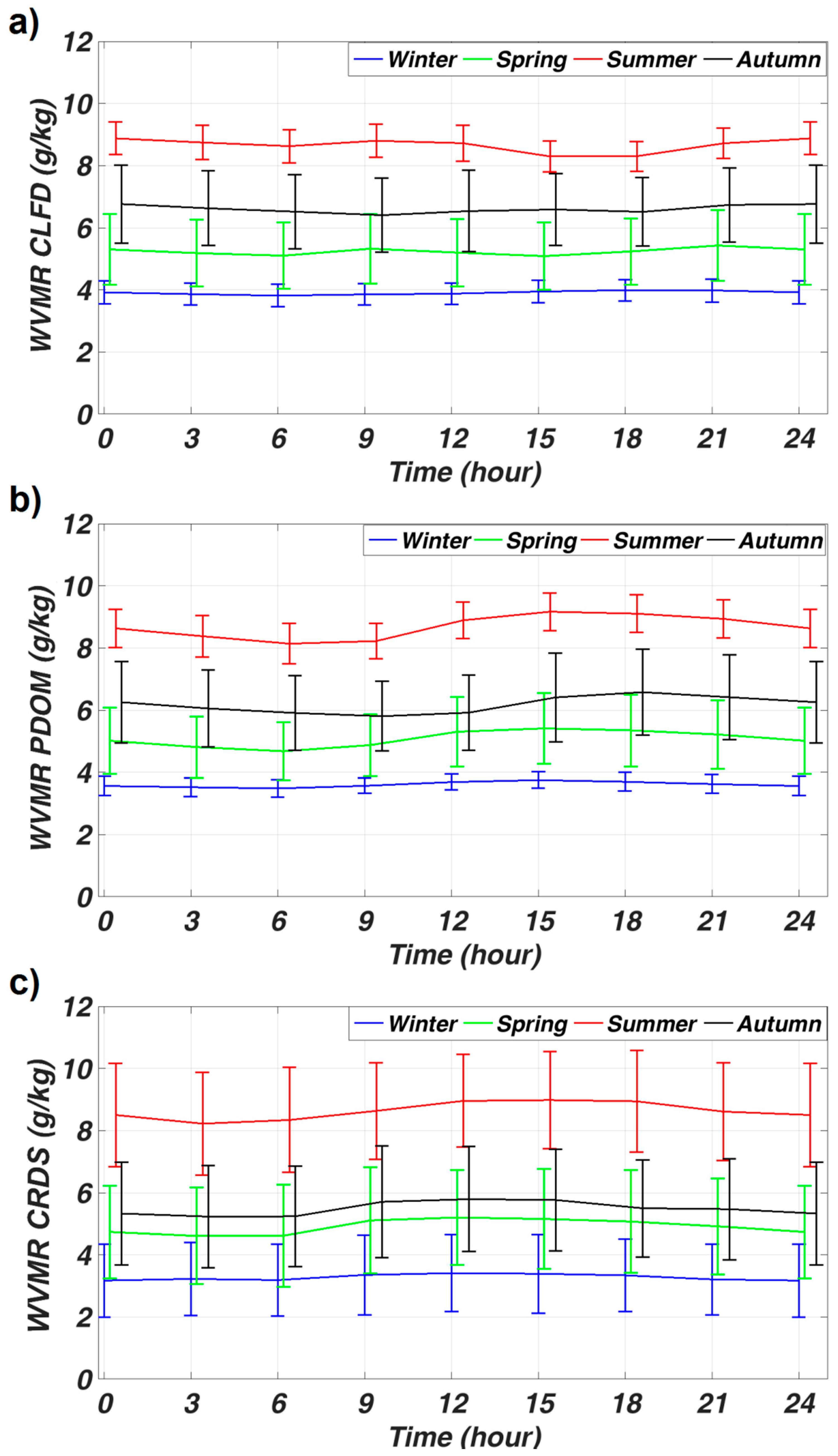
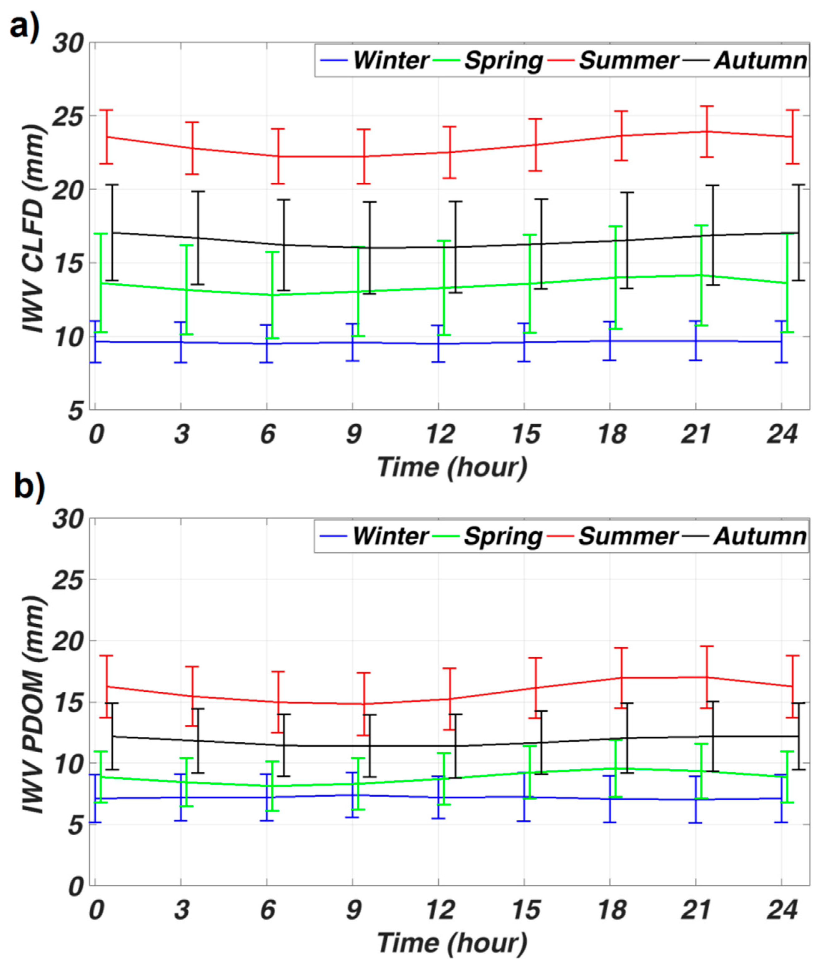
4.1. Surface Water Vapor

In addition to carbon dioxide, variations of water vapor at the interface between the earth’s surface and the atmosphere play an important role in the functioning of ecosystems [53]. It is therefore important to characterize the variations and cycles of water vapor near the surface. Figure 3 illustrates the seasonal and daily variations of surface WVMR at Cézeaux and puy de Dôme. The annual cycle of water vapor is clearly established for both sites and all types of measurements. The maximum of water vapor is observed in summer (June to August) and the minimum in winter (December to February), and autumn (September to November) is slightly wetter than spring (March to May). The seasonal means of WVMR are given in Table 2.
The mean surface WVMR calculated for each season from the meteorological station at Cézeaux is very close to ones from the meteorological station at puy de Dôme. Generally, the average of WVMR decreases with altitude, and water vapor concentrates in the low troposphere. This has been observed at different locations from radiosoundings and lidar [54,55,56]. Here we do not observe this vertical decrease of water vapor between the meteorological station at Cézeaux (423 m) and those of puy de Dôme (1463 m). The CO-PDD sites are affected by dominant westerly winds from oceanic origin [57], and we suggest that foehn local processes dehydrates the air at Clermont-Ferrand compared to puy de Dôme, after getting over the puy chain reliefs. This dynamical process has been studied for other mountain chains, for example over the Andes [58] or the Pyrenees [59].

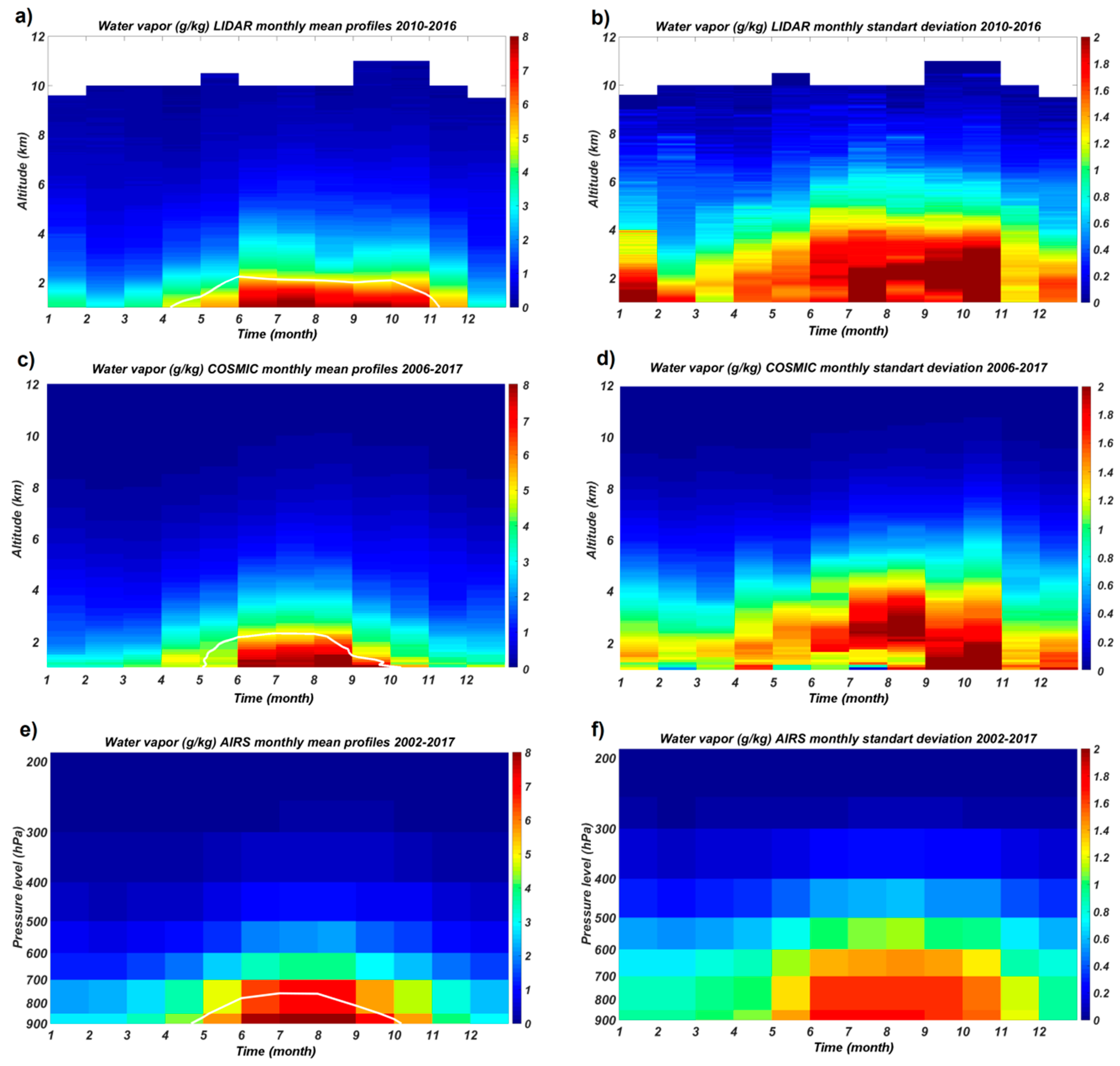
4.2. Vertical Columns and Profiles

The variability of surface water vapor illustrated by standard deviation is similar for puy de Dôme and Cézeaux meteorological stations. It is larger in autumn and spring (more than 1 g·kg−1) than summer (0.6 g·kg−1) and winter (0.3 g·kg−1). The CRDS data presents slightly larger variability (between 1.2 and 1.7 g·kg−1), but the series are shorter (less than two years). Two years meteorological stations data series show a variability of the same order of magnitude than the CRDS series.
The two sites present almost no diurnal cycle. That suggests that the variability of surface water vapor at this site is more influenced by sporadic meteorological systems than by regular diurnal variations.
The CO-PDD sites are equipped with remote sensing instruments providing total columns and vertical profiles of water vapor. In this section, we document the variability of IWV at Cézeaux and puy de Dôme as seen by the different techniques presented in Section 2 and Section 3.
Figure 4 illustrates the seasonal and daily variability of IWV at Cézeaux and puy de Dôme. Similarly to surface observations, a strong seasonal cycle is observed on the two sites: at Cézeaux the average values are between 23 mm in summer and 9.6 mm in winter, and at puy de Dôme, the average values are between 15.9 mm in summer and 7.2 mm in winter. The differences of IWV content between the two sites are 7 mm (30% of puy de Dôme IWV), 4.7 mm (28%), 4.7 mm (34%), and 2.4 mm (25%) for respectively summer, autumn, spring, and winter. This result shows that the foehn effect we mentioned in Section 4.1 does not affect significantly the total column, as observed in the Swiss Alps [60].
We do not observe a significant daily cycle. Similarly to surface observations, the variability is slightly higher in spring and autumn, compared to summer and winter, and comparable for puy de Dôme and Cézeaux. This result is slightly different to those observed above Zugspitze (Garmisch-Partenkirchen, Germany, 2962 m above sea level), where the variability is larger in summer [61]. Recently, the diurnal cycle of water vapor has been determined from the GPS ground network in the Volga-Ural region of Russia by Kalinnikov and Khutorova [62], who showed also maximal amplitude of the diurnal harmonics in summer for stations located on the windward side of mountains.
Figure 5 presents the monthly mean and standard deviation of WVMR profiles from lidar, compared with two satellite products, COSMIC and AIRS.
The annual cycle of water vapor (maximum values in summer and minimum in winter) observed on GPS IWV is occurring over the whole troposphere until the tropopause (near 12 km), and is similar for the three datasets, in amplitude and altitude. In addition, the three datasets highlight a larger monthly variability in the lower layers than in the free troposphere and in summer than in winter. One difference we can observe is that the monthly variability is larger for the lidar dataset, than COSMIC, and finally AIRS.
This higher variability of the lidar dataset can be explained by the fact that the series do not cover the same period, and lidar measures water vapor very locally, while COSMIC and AIRS probe a larger part of the atmosphere. A part of the differences in the variability could also be attributed to the difference of vertical resolution and the number of observations.
The 5 g·kg−1 isocontours altitude is near 2 km in summer, and less than 1 km in winter. Farah et al. [63] used several different approaches to determine the boundary layer height, and showed that the boundary layer varies from 400 m to 2500 m, with important daily and seasonal variations. A more precise comparison with water vapor profiles could provide additional elements to determine the boundary layer height for this site.

5. Geophysical Forcing Contributions

We present the estimation of the influence of the geophysical forcings on water vapor variations using the methodology described in Section 3.3. Table 3 presents the contributions and incertitudes for the semi-annual cycle, annual cycle, EA, EA_WR and NAO forcings for the different observation series: WVMR at the meteorological site of puy de Dôme between 2011 and 2017, WVMR at the meteorological site of Cézeaux between 2004 and 2017 IWV at the meteorological site of Cézeaux between 2009 and 2016, and WVMR deduced from the satellite AIRS at 850 hPa on the most closed point of Cézeaux between 2003 and 2016.
All values of coefficients determination are higher than 92.8%. This shows that the regression model explains correctly the variability of the water vapor over time. As expected, the annual cycle is the dominant component in all the studied parameters. The annual cycle is found to explain 57% of the variation of water vapor for all the studied parameters, with a maximum value of 65.6 ± 1% for AIRS WMMR.
EA and EA-WR have a strong impact on the coupling between the sub-tropical Atlantic Jet and the African Jet, which in turn affects the climate variability over Europe [46]. A strong contribution of EA-WR and EA at the variability of water vapor at Clermont-Ferrand is observed. Each forcing contributes for all parameters more than 10.9 ± 3.1% except for EA-WR that has a negative contribution (−5.1 ± 4.0%) for AIRS WVMR. That means that EA-WR and WVMR AIRS are in phase opposition.
NAO dictates climate variability from the eastern seaboard of the United States to Siberia and from the Arctic to the subtropical Atlantic, especially during winter. It strongly affects water management [64]. The contribution of NAO on the variability of water vapor in Clermont-Ferrand is not significant, except for AIRS WVMR (4.6 ± 3.6%). This is a quite surprising result because the back trajectory analysis shows that the dominant air mass origins are West (54%), followed by North (18%), then East (15%) and South (13%) [9]. We thought that the oceanic westerly air masses should be correlated with a greater influence of the NAO on the water vapor trends observed at Cézeaux and puy de Dôme, but this is not the case here. Recently, Pope et al., 2018 [65] used satellite observations and a chemistry transport model to investigate the influence of NAO on European tropospheric pollutants. They show that NAO circulation patterns are an important governing factor for European wintertime composition and air pollution. Wypych et al. 2018 [66] confirmed the significance of atmospheric circulation in the formation of moisture content in the winter season, but its markedly lower impact in other seasons. The relationships are characterized by statistically significant spatial differentiation. In this study CO-PDD is near the limit of two different regions, mid-Atlantic and mid-continental, with a possible role of local factors impacting moisture content. This could explain why the demonstration of the influence of NAO on the long series of water vapor observation is difficult to highlight with our multi regression approach.

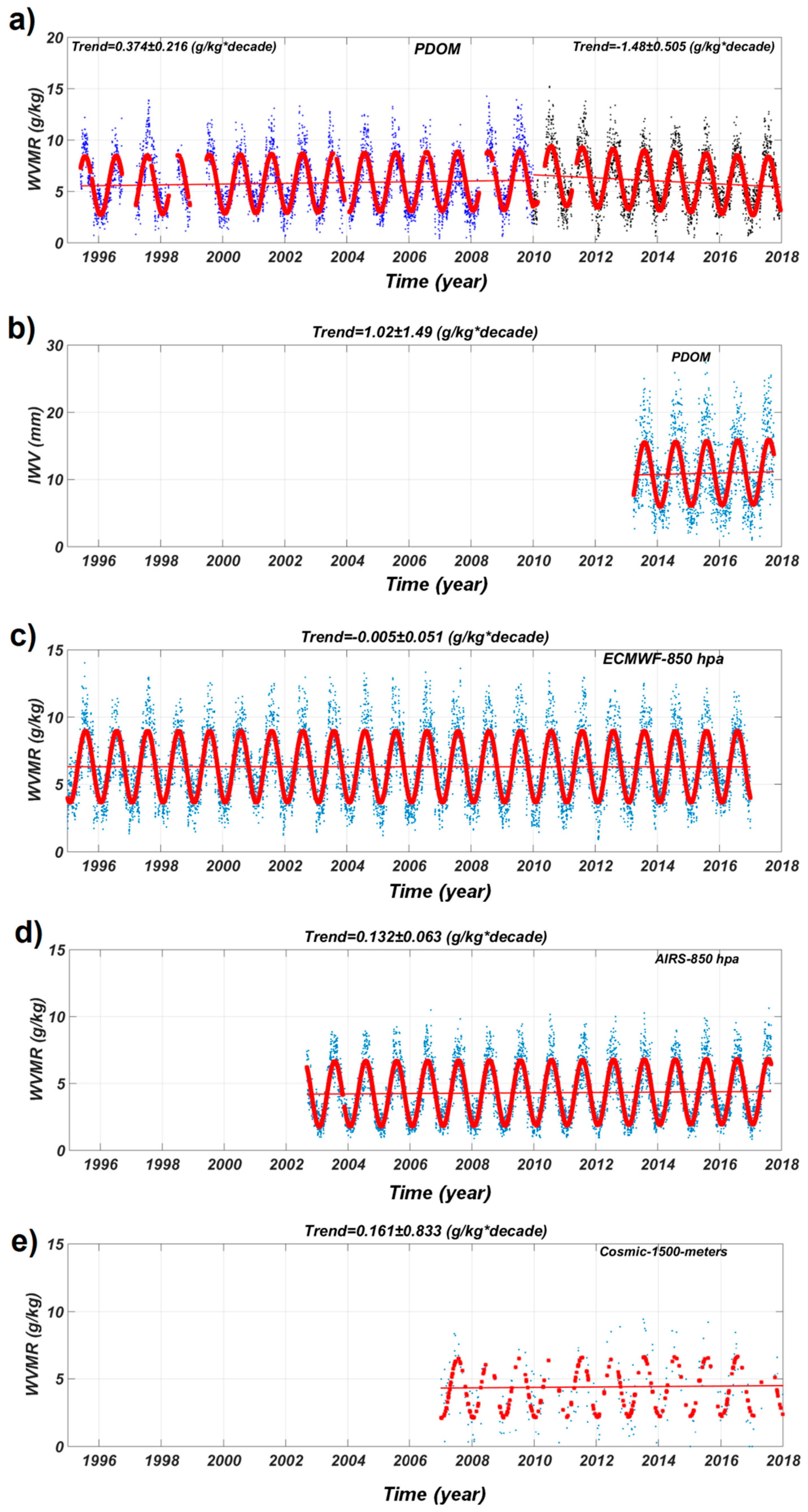
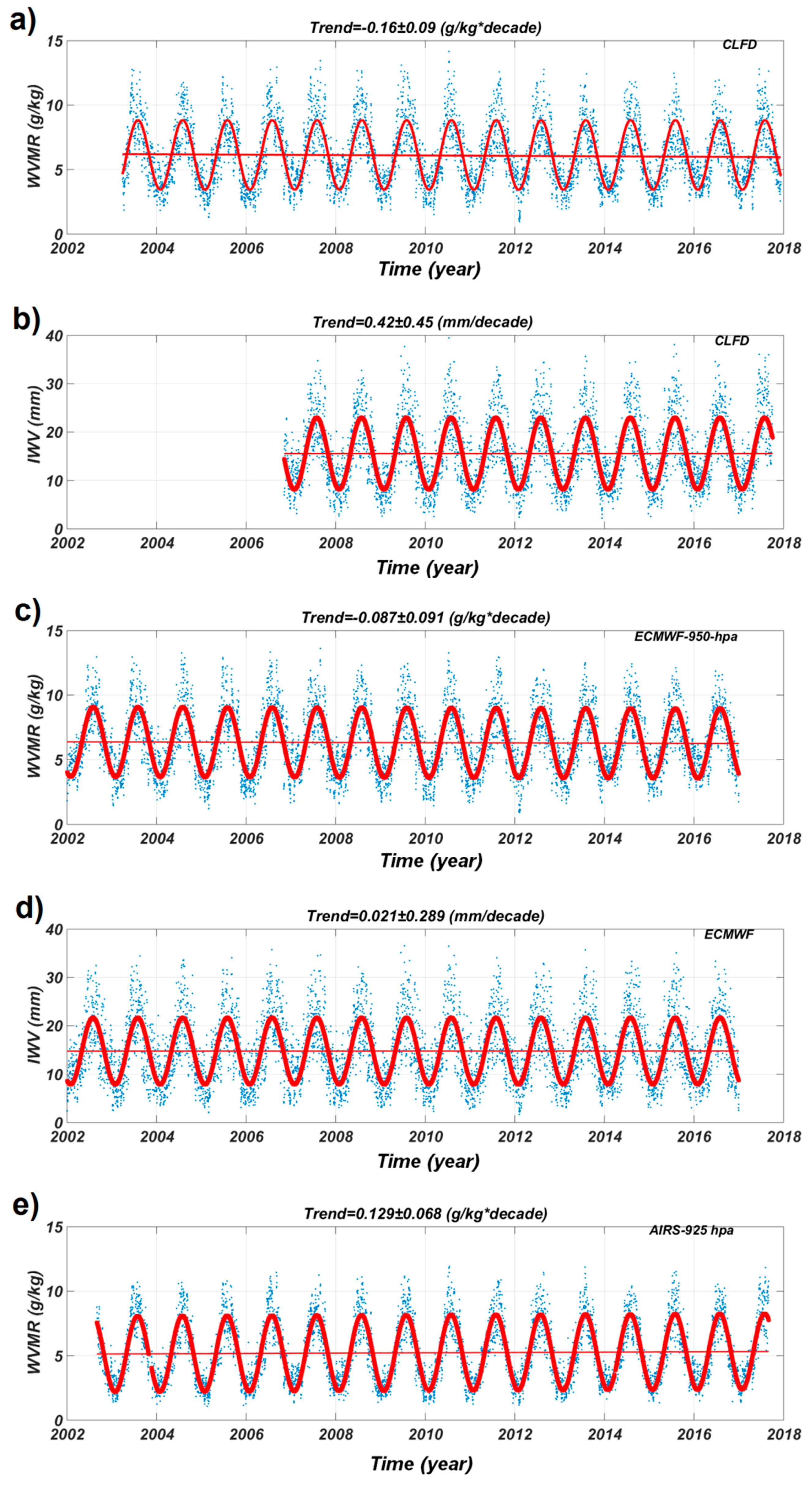
6. Decadal Trends from Long Time Series of Water Vapor

The time period covered by the dataset makes it possible to envisage a first estimate of decadal trends. Figure 6 illustrates the variations, annual cycles, and trends of WVMR at the meteorological site of Cézeaux between 2002 and 2018, GPS IWV at the meteorological site of Cézeaux between 2007 and 2018, specific humidity at 925 hPa and IWV deduced from ECMWF ERA-Interim also between 2002 and 2018, and WVMR deduced from AIRS at 925 hPa between 2002 and 2018.
GPS IWV presents a positive trend at the site of Cézeaux: 0.42 ± 0.45 mm/decade, but ECMWF ERA-Interim presents almost no trend: 0.02 ± 0.29 mm/decade. Sussmann et al. [67] found also positive trends for observations of IWV in Zugspitze Germany (47° N, 11° E, 2964 m above sea level), 0.79 ± 0.14 mm/decade between 1996 and 2008. Ning et al. [68] calculated also trends of IWV at 101 GPS sites. Trends in all the 101 sites present a large variability, between −0.67 ± 0.34 mm/decade at Tibb (38° N, −122° E) and 1.03 ± 0.78 mm/decade at Coco (−12° N, 96° E). The closest site from Cézeaux is Zimm (47° N, 7.5° E), whose trend is 0.18 ± 0.18 mm/decade. Compared to these values, the trends observed at Cézeaux are inside the range of the global scale study of Ning et al. [68].
Nilsson et al. [69] also present a 10 year ground-based GPS trend estimation in Finland and Sweden. The linear trends in the IWV are between −0.2 and +1.0 mm/decade. Haas et al. [70] present long term trends (30 years) in the amount of atmospheric water vapor at the Swedish West coast derived from four different techniques; very long baseline interferometry, GPS, ground-based microwave radiometry, and radiosondes. The four techniques detect individual IWV positive trends on the order of 0.37 ± 0.02 mm/decade to 0.62 ± 0.04 mm/decade. The trends observed at Cézeaux are inside the range of the values of Ning et al. [64] and Nilsson et al. [65].
The WVMR trend deduced from AIRS at 925 hPa is 0.13 ± 0.07 g·kg−1/decade, but WVMR deduced from the meteorological station at Cézeaux present a negative trend: −0.16 ± 0.09 g·kg−1/decade. If many authors present trend estimates from the vertical columns of water vapor, very few present trend estimates for ground based WVMR. Thao et al. [71] studied the local linear trends of water vapor monthly anomalies over oceans between 2004 and 2010 using 4 sources of data: Advanced Microwave Scanning Radiometer for Earth Observing System (AMSR-E), Jason-1 microwave radiometer (JMR), Enlist microwave radiometer (MWR), and ECMWF ERA-Interim. The linear trend of water vapor above the border section with France from the Atlantic Ocean is between 0 and −0.2 mm/decade, which is in agreement with the negative trend obtained from the meteorological station at Cézeaux. WVMR trend at 950 hPa deduced from ECMWF ERA-Interim on the most closed point of Cézeaux is also negative: −0.09 ± 0.09 g·kg−1/decade.
Figure 7 illustrates the variations, annual cycles, and trends at puy de Dôme: WVMR at the meteorological station at puy de Dôme between 1995 and 2018, GPS IWV at puy de Dôme between 2013 and 2018, ECMWF ERA-Interim and AIRS WVMR at 850 hPa.
IWV data at puy de Dôme is available between 2013 and 2018. This period is too short to establish a decadal trend. We have identified a discontinuity in 2010 in the series of WVMR from the meteorological station at puy de Dôme, corresponding to a displacement of the instrument of about twenty meters during the renovation of the puy de Dôme station, combined with a sensor change. Then we have separated the series in two parts: after and before 2010.
WVMR deduced from ECMWF ERA-Interim specific humidity at 850 hPa presents almost no trend: −0.005 ± 0.051 g·kg−1/decade. WVMR at the meteorological station at puy de Dôme presents a positive trend in the first part until 2010 (0.38 ± 0.22 g·kg−1/decade) and a negative trend after 2010 (−1.48 ± 0.51 g·kg−1/decade). AIRS shows a positive WVMR trend at 850 hPa (0.132 ± 0.063 g·kg−1/decade) close to the trend observed at 925 hPa (0.129 ± 0.068 g·kg−1/decade), due to the low vertical resolution of the instrument. In the study of Thao et al. [67], the regional trends between 2004 and 2010 in the eastern part of the North Atlantic Ocean are also quite uncertain and dependent on the datasets analyzed. Trend of WVMR detected by AIRS at 850 hPa is equal to 0.13 ± 0.06 g·kg−1/decade. The vertical level 1500 m of COSMIC shows also a positive trend, but non-significant because of the small number of points.
At the end, the trend results can be summarized as follows:
  • At the Cezeaux site, the trend of IWV (2007–2017) is positive but not significant and the trend of WVMR (2003–2017) is negative.
  • At the puy de Dôme site, the trends are difficult to analyze because the series are temporally short or inhomogeneous.
  • Trends of IWV and specific humidity of ECMWF ERA-Interim are weaker than trends calculated from observation series.
  • AIRS WVMR trends are in disagreement with ECMWF and the meteorological sensor WVMR trends, probably due to the low vertical resolution of AIRS.

7. Conclusions

In this study we presented an analysis of a long data set of lidar, GPS, CRDS, and meteorological observations at the sites of puy de Dôme and Cezeaux. We compare the variability, cycles and long term trends to the ECMWF ERA-Interim reanalysis, AIRS, and Cosmic satellites.
WVMR CRDS data are very well correlated with the WVMR data of the meteorological station at puy de Dôme (R2 = 0.98). The WVMR at puy de Dôme reaches its maximum in summer (8.9 g·kg−1), and its minimum in winter (3.6 g·kg−1), and autumn is slightly wetter than spring. Data show a daily variability larger in summer than in winter, but almost no daily cycle (less than 1 g·kg−1). That suggests that the variability of surface water vapor at this site is more influenced by sporadic meteorological systems than by regular diurnal variations. WVMR observed at the site of puy de Dôme are close to those observed at Cézeaux, despite the difference of altitude between the two sites (around 1000 m). CO-PDD is under the influence of dominant westerly winds from oceanic origin, and we suggest that foehn local processes dehydrate the air close to the surface at Clermont-Ferrand compared to puy de Dôme, after getting over the puy chain reliefs. This dynamical process has been studied for other mountain chains, for example over the Andes [56] or the Pyrenees [57]. The foehn local process seems to have an impact only on the low layers as the IWV at puy de Dôme are lower than those measured at Cézeaux.
The analysis of lidar and satellite vertical profiles shows that the monthly variability is larger for the Lidar dataset than satellite products used in this study (COSMIC and AIRS). Given the high variability of water vapor and the limited time coverage of the datasets, the decadal trends are difficult to establish using these data sets.
The IWV trend at the Cezeaux site is positive but not significant and the trend of WVMR is negative. At the puy de Dôme site, the trends are difficult to analyze because the series are temporally short or inhomogeneous. The trends of IWV and specific humidity from ERA-Interim reanalysis are weaker than trends calculated from the observation series.
The analysis of geophysical forcings shows that EA and the EA-WR are the most influent on tropospheric water vapor distributions. NAO dictates climate variability from the eastern seaboard of the United States to Siberia and from the Arctic to the subtropical Atlantic, especially during winter. It strongly affects water management, but this effect is not verified by the contribution of NAO on the variability of water vapor in Clermont-Ferrand. This is quite a surprising result because backtrajectory analyses show that dominant air masses come from West (53%), and are from oceanic origin.
In the future, we will continue to investigate variability and trends of water vapor on the CO-PDD sites. It would be interesting to couple the evolution of water vapor to geophysical mechanisms influencing water vapor, such as stratosphere-troposphere exchanges and precipitation events, through case studies or a more sophisticated statistical approach.

Author Contributions

Conceptualization, D.H. and J.-L.B.; Funding acquisition, J.V.B.; Investigation, J.-L.B. and N.M.; Methodology, D.H., J.-L.B. and N.M.; Resources, J.-L.B., P.F., J.-M.P., P.B., M.R. and C.Y.K.; Software, D.H., J.-L.B., N.B. and V.D.; Writing–original draft, D.H. and J.-L.B.; Writing–review & editing, N.M., J.V.B., P.F., J.-M.P., P.B., M.R., C.Y.K., N.B. and V.D.

Funding

This research is based on data from CO-PDD data, which is supported by the University Clermont-Auvergne (UCA), by the French institute for research (CNRS-INSU), and by the French space national center (CNES).

Acknowledgments

We acknowledge ECMWF, CDAAC, the NASA’s Earth-Sun System Division and the Goddard Earth Sciences (GES) Data and Information Services Center (DISC) Distributed Active Archive Center (DAAC) for providing ERA-Interim reanalysis and COSMIC and AIRS observations. We acknowledge the technical staff of LaMP/OPGC for their work on the puy de Dôme and Cézeaux instrumentations.

Conflicts of Interest

The authors declare no conflict of interest.

References

  1. Twomey, S. Aerosols, clouds and radiation. Atmos. Environ. 1991, 25, 2435–2442. [Google Scholar] [CrossRef]
  2. Lawson, R.P.; Angus, L.J.; Heymsfield, A.J. Cloud Particle Measurements in Thunderstorm Anvils and Possible Weather Threat to Aviation. J. Aircr. 1998, 35, 113–121. [Google Scholar] [CrossRef]
  3. IPCC. Climate Change 2013: The Physical Science Basis; Contribution of Working Group I to the Fifth Assessment Report of the Intergovernmental Panel on Climate Change; Cambridge University Press: Cambridge, UK; New York, NY, USA, 2013. [Google Scholar]
  4. Trenberth, K.E.; Stepaniak, D.P. Seamless Poleward Atmospheric Energy Transports and Implications for the Hadley Circulation. J. Clim. 2003, 16, 3706–3722. [Google Scholar] [CrossRef]
  5. D’Aulerio, P.; Fierli, F.; Congeduti, F.; Redaelli, G. Analysis of water vapor LIDAR measurements during the MAP campaign: Evidence of sub-structures of stratospheric intrusions. Atmos. Chem. Phys. 2005, 5, 1301–1310. [Google Scholar] [CrossRef]
  6. Baray, J.-L.; Pointin, Y.; van Baelen, J.; Lothon, M.; Campistron, B.; Cammas, J.-P.; Masson, O.; Colomb, A.; Hervier, C.; Bezombes, Y.; et al. Case study and climatological analysis of upper tropospheric jet stream and stratosphere-troposphere exchanges using VHF profilers and radionuclide measurements in France. J. Appl. Meteorol. Climatol. 2017, 56, 3081–3097. [Google Scholar] [CrossRef]
  7. Bojinski, S.; Verstraete, M.; Peterson, T.C.; Richter, C.; Simmons, A.; Zemp, M. The Concept of Essential Climate Variables in Support of Climate Research, Applications, and Policy. Bull. Am. Meteorol. Soc. 2014, 95, 1431–1443. [Google Scholar] [CrossRef] [Green Version]
  8. Wulfmeyer, V.; Hardesty, R.M.; Turner, D.D.; Behrendt, A.; Cadeddu, M.P.; di Girolamo, P.; Schlüssel, P.; van Baelen, J.; Zus, F. A review of the remote sensing of lower tropospheric thermodynamic profiles and its indispensable role for the understanding and the simulation of water and energy cycles. Rev. Geophys. 2015, 53, 819–895. [Google Scholar] [CrossRef] [Green Version]
  9. Noh, Y.-C.; Sohn, B.-J.; Kim, Y.; Joo, S.; Bell, W. Evaluation of Temperature and Humidity Profiles of Unified Model and ECMWF Analyses Using GRUAN Radiosonde Observations. Atmosphere 2016, 7, 94. [Google Scholar] [CrossRef]
  10. Colomb, A.; Baray, J.L.; Sellegri, K.; Freney, E.; Deguillaume, L.; Pichon, J.M.; Ribeiro, M.; Bouvier, L.; Picard, D.; Van Baelen, J.; et al. The instrumented station Cézeaux-Opme-Puy De Dôme (CO-PDD): 20 years of measurement to document the atmospheric composition and climate change. 2018. to be submitted. [Google Scholar]
  11. Zhao, P.; Yin, Y.; Xiao, H.; Zhou, Y.; Liu, J. Role of water vapor content in the effects of aerosol on the electrification of thunderstorms: A numerical study. Atmosphere 2016, 7, 137. [Google Scholar] [CrossRef]
  12. Available online: http://wwwobs.univ-bpclermont.fr/SO/mesures/index.php (accessed on 31 July 2018).
  13. Available online: https://www.vaisala.com/sites/default/files/documents/HMP45AD-User-Guide-U274EN.pdf (accessed on 31 July 2018).
  14. Hyland, R.W.; Wexler, A. Formulations for the Thermodynamic Properties of the saturated Phases of H2O from 173.15K to 473.15K. ASHRAE Trans. 1983, 89, 500–519. [Google Scholar]
  15. Todd, M.W.; Provencal, R.A.; Owano, T.G.; Paldus, B.A.; Kachanov, A.; Vodopyanoy, K.L.; Hunter, M.; Coy, S.L.; Arnold, J.T. Application of mid-infrared cavity-ringdown spectroscopy to trace explosives vapor detection using a btoadly tunable (6–8 µm) optical parametric oscillator. Appl. Phys. B 2002, 75, 367–376. [Google Scholar] [CrossRef]
  16. Winderlich, J.; Chen, H.; Gerbig, C.; Seifert, T.; Kolle, O.; Lavric, J.V.; Kaiser, C.; Höfer, A.; Heimann, M. Continuous low-maintenance CO2/CH4/H2O measurements at the Zotino Tall Tower Observatory (ZOTTO) in Central Siberia. Atmos. Meas. Tech. 2010, 3, 1113–1128. [Google Scholar] [CrossRef]
  17. Rella, C.W.; Chen, H.; Andrews, A.E.; Filges, A.; Gerbig, C.; Hatakka, J.; Karion, A.; Miles, N.L.; Richardson, S.J.; Steinbacher, M.; et al. High accuracy measurements of dry mole fractions of carbon dioxide and methane in humid air. Atmos. Meas. Tech. 2013, 6, 837–860. [Google Scholar] [CrossRef]
  18. Available online: http://rgp.ign.fr (accessed on 31 July 2018).
  19. Zumberge, J.F.; Heflin, M.B.; Jefferson, D.C.; Watkins, M.M.; Webb, F.H. Precise point positioning for the efficient and robust analysis of GPS data from large networks. J. Geophys. Res. 1997, 102, 5005–5017. [Google Scholar] [CrossRef] [Green Version]
  20. Petit, G.; Luzum, B. IERS Conventions. IERS Technical, Note No. 36, 2010, ISSN 1019-4568. Available online: http://www.iers.org/TN36/ (accessed on 31 July 2018).
  21. Lyard, F.; Lefevre, F.; Letellier, T.; Francis, O. Modelling the global ocean tides: Modern insights from FES2004. Ocean Dyn. 2006, 56, 394. [Google Scholar] [CrossRef]
  22. Bertiger, W.; Desai, S.D.; Haines, B.; Harvey, N.; Moore, A.W.; Owen, S.; Weiss, J.P. Single receiver phase ambiguity resolution with GPS data. J. Geod. 2010, 84, 327. [Google Scholar] [CrossRef]
  23. Boehm, J.; Niell, A.; Tregoning, P.; Schuh, H. Global Mapping Function (GMF): A new empirical mapping function based on numerical weather model data. Geophys. Res. Lett. 2006, 33, L07304. [Google Scholar] [CrossRef]
  24. Bosser, P.; Bock, O.; Thom, C.; Pelon, J.; Willis, P. A case study of using Raman lidar measurements in high-accuracy GPS applications. J. Geod. 2010, 84, 251. [Google Scholar] [CrossRef]
  25. Bock, O.; Bosser, P.; Bourcy, T.; David, L.; Goutail, F.; Hoareau, C.; Keckhut, P.; Legain, D.; Pazmino, A.; Pelon, J.; et al. Accuracy assessment of water vapor measurements from in situ and remote sensing techniques during the DEMEVAP 2011 campaign at OHP. Atmos. Meas. Tech. 2013, 6, 2777–2802. [Google Scholar] [CrossRef] [Green Version]
  26. Bevis, M.; Businger, S.; Herring, T.A.; Rocken, C.; Anthes, R.A.; Ware, R.H. GPS Meteorology: Remote Sensing of Atmospheric Water Vapor Using the Global Positioning System. J. Geophys. Res. 1992, 97, 15787–15801. [Google Scholar] [CrossRef]
  27. Fréville, P.; Montoux, N.; Baray, J.-L.; Chauvigné, A.; Réveret, F.; Hervo, M.; Dionisi, D.; Payen, G.; Sellegri, K. Lidar developments at Clermont-Ferrand—France for atmospheric observation. Sensors 2015, 15, 3041–3069. [Google Scholar] [CrossRef] [PubMed]
  28. Parkinson, C.L. Aqua: An Earth-Observing Satellite Mission to Examine Water and Other Climate Variables. IEEE Trans. Geosci. Remote Sens. 2003, 41, 173–183. [Google Scholar] [CrossRef]
  29. Available online: http://docserver.gesdisc.eosdis.nasa.gov/repository/Mission/AIRS/3.3_ScienceDataProductDocumentation/3.3.4_ProductGenerationAlgorithms/V6_L2_Product_User_Guide.pdf (accessed on 31 July 2018).
  30. Kursinski, E.R.; Hajj, G.A.; Hardy, K.R.; Schofield, J.T.; Linfield, R. Observing Earth’s atmosphere with radio occultation measurements. J. Geophys. Res. 1997, 102, 429–465. [Google Scholar] [CrossRef]
  31. Anthes, R.A.; Bernhardt, P.A.; Chen, Y.; Cucurull, L.; Dymond, K.F.; Ector, D.; Healy, S.B.; Ho, S.; Hunt, D.C.; Kuo, Y.; et al. The COSMIC/FORMOSAT-3 Mission: Early Results. Bull. Am. Meteor. Soc. 2008, 89, 313–334. [Google Scholar] [CrossRef] [Green Version]
  32. Isioye, O.A.; Combrinck, L.; Botai, J.O.; Munghemezulu, C. The Potential for Observing African Weather with GNSS Remote Sensing. Adv. Meteorol. 2015, 723071. [Google Scholar] [CrossRef]
  33. Ho, S.-P.; Peng, L.; Anthes, R.A.; Kuo, Y.-H.; Lin, H.-C. Marine Boundary Layer Heights and Their Longitudinal, Diurnal, and Interseasonal Variability in the Southeastern Pacific Using COSMIC, CALIOP, and Radiosonde Data. J. Clim. 2015, 28, 2856–2872. [Google Scholar] [CrossRef]
  34. Davis, N.A.; Birner, T. Seasonal to multidecadal variability of the width of the tropical belt. J. Geophys. Res. 2013, 118, 7773–7787. [Google Scholar] [CrossRef] [Green Version]
  35. Gettelman, A.; Wang, T. Structural diagnostics of the tropopause inversion layer and its evolution. J. Geophys. Res. 2015, 120, 46–62. [Google Scholar] [CrossRef] [Green Version]
  36. Dee, D.P.; Uppala, S.M.; Simmons, A.J.; Berrisford, P.; Poli, P.; Kobayashi, S.; Bechtold, P. The ERA-Interim reanalysis: Configuration and performance of the data assimilation system. Q. J. R. Meteorol. Soc. 2011, 137, 553–597. [Google Scholar] [CrossRef]
  37. Available online: http://apps.ecmwf.int/datasets/data/interim-full-daily (accessed on 31 July 2018).
  38. Mastenbrook, H.J. The variability of water vapor in the stratosphere. J. Atmos. Sci. 1971, 28, 1495–1501. [Google Scholar] [CrossRef]
  39. Available online: ftp://ftp.cpc.ncep.noaa.gov/wd52dg/data/indices/tele_index.nh (accessed on 31 July 2018).
  40. Lamb, P.J.; Peppler, R.A. North Atlantic Oscillation: Concept and application. Bull. Am. Meteorol. Soc. 1987, 68, 1218–1225. [Google Scholar] [CrossRef]
  41. Hurrell, J.W.; van Loon, H. Decadal variations in climate associated with the North Atlantic Oscillation. Clim. Chang. 1997, 36, 301–326. [Google Scholar] [CrossRef]
  42. Wibig, J. Precipitation in Europe in relation to circulation patterns at the 500 hPa level. Int. J. Climatol. 1999, 19, 253–269. [Google Scholar] [CrossRef] [Green Version]
  43. Jerez, S.; Jimenez-Guerrero, P.; Montávez, J.P.; Trigo, R.M. Impact of the North Atlantic Oscillation on European aerosol ground levels through local processes: A seasonal model-based assessment using fixed anthropogenic emissions. Atmos. Chem. Phys. 2013, 13, 11195–11207. [Google Scholar] [CrossRef]
  44. Wallace, J.M.; Gutzler, D.S. Teleconnections in the geopotential height field during the Northern Hemisphere winter. Mon. Weather Rev. 1981, 109, 784–812. [Google Scholar] [CrossRef]
  45. Comas-Bru, L.; McDermott, F. Impacts of the EA and SCA patterns on the European twentieth century NAO–winter climate relationship. Q. J. R. Meteorol. Soc. 2014, 140, 354–363. [Google Scholar] [CrossRef]
  46. Barnston, A.G.; Livezey, R.E. Classification, Seasonality and Persistence of Low-Frequency Atmospheric Circulation Patterns. Mon. Weather Rev. 1987, 115, 1083–1126. [Google Scholar] [CrossRef] [Green Version]
  47. Krichak, S.O.; Alpert, P. Decadal trends in the east Atlantic–west Russia pattern and Mediterranean precipitation. Int. J. Climatol. 2005, 25, 183–192. [Google Scholar] [CrossRef]
  48. Ionita, M. The Impact of the East Atlantic/Western Russia Pattern on the Hydroclimatology of Europe from Mid-Winter to Late Spring. Climate 2014, 2, 296–309. [Google Scholar] [CrossRef] [Green Version]
  49. Beaufils, D.; Richoux, H.; Pagnol, L.M. Régression linéaire et incertitudes expérimentales. Bull. Union Phys. 1997, 796, 1361–1376. [Google Scholar]
  50. Keckhut, P.; Hauchecorne, A.; Chanin, M.L. Midlatitude long-term variability of the middle atmosphere: Trends and cyclic and episodic changes. J. Geophys. Res. 1995, 100, 18887–18897. [Google Scholar] [CrossRef]
  51. Bègue, N.; Bencherif, H.; Sivakumar, V.; Kirgis, G.; Mzé, N.; Leclair de Bellevue, J. Temperature variability and trends in the UT-LS over a subtropical site: Reunion (20.8° S, 55.5° E). Atmos. Chem. Phys. 2010, 10, 8563–8574. [Google Scholar] [CrossRef] [Green Version]
  52. Toihir, A.M.; Portafaix, T.; Sivakumar, V.; Bencherif, H.; Pazmiño, A.; Bègue, N. Variability and trend in ozone over the southern tropics and subtropics. Ann. Geophys. 2018, 36, 381–404. [Google Scholar] [CrossRef] [Green Version]
  53. Baldocchi, D.; Falge, E.; Gu, L.; Olson, R.; Hollinger, D.; Running, S.; Anthoni, P.; Bernhofer, C.; Davis, K.; Evans, R.; et al. FLUXNET: A new tool to study the temporal and spatial variability of ecosystem–scale carbon dioxide, water vapor, and energy flux densities. Bull. Am. Meteorol. Soc. 2001, 82, 2415–2434. [Google Scholar] [CrossRef]
  54. Goldsmith, J.E.M.; Bisson, S.E.; Ferrare, R.A.; Evans, K.D.; Whiteman, D.N.; Melfi, S.H. Raman lidar profiling of atmospheric water vapor: Simultaneous measurements with two collocated systems. Bull. Am. Meteorol. Soc. 1994, 75, 975–982. [Google Scholar] [CrossRef]
  55. Ferrare, R.A.; Melfi, S.H.; Whiteman, D.N.; Evans, K.D.; Schmidlin, F.J.; Starr, D.O. A Comparison of Water Vapor Measurements Made by Raman Lidar and Radiosondes. J. Atmos. Ocean. Technol. 1995, 12, 1177–1195. [Google Scholar] [CrossRef] [Green Version]
  56. Hoareau, C.; Keckhut, P.; Baray, J.-L.; Robert, L.; Courcoux, Y.; Porteneuve, J.; Vömel, H.; Morel, B. A Raman lidar at La Reunion (20.8° S, 55.5° E) for monitoring water vapour and cirrus distributions in the subtropical upper troposphere: Preliminary analyses and description of a future system. Atmos. Meas. Tech. 2012, 5, 1333–1348. [Google Scholar] [CrossRef] [Green Version]
  57. Deguillaume, L.; Charbouillot, T.; Joly, M.; Vaïtilingom, M.; Parazols, M.; Marinoni, A.; Amato, P.; Delort, A.-M.; Vinatier, V.; Flossmann, A.I.; et al. Classification of clouds sampled at the puy de Dôme (France) based on 10 yr of monitoring of their physicochemical properties. Atmos. Chem. Phys. 2014, 14, 1485–1506. [Google Scholar] [CrossRef] [Green Version]
  58. Seluchi, M.E.; Norte, F.A.; Satyamurty, P.; Chou, S.C. Analysis of three situations of the foehn effect over the Andes (zonda wind) using the Eta–CPTEC regional model. Weather Forecast. 2003, 18, 481–501. [Google Scholar] [CrossRef]
  59. Dione, C.; Lohou, F.; Chiriaco, M.; Lothon, M.; Bastin, S.; Baray, J.-L.; Yiou, P.; Colomb, A. The influence of synoptic circulations and local processes on temperature anomalies at three French observatories. J. Atmos. Ocean. Technol. 2017, 56, 141–158. [Google Scholar] [CrossRef]
  60. Morland, J.; Mätzler, C. Spatial interpolation of GPS integrated water vapour measurements made in the Swiss Alps. Meteorol. Appl. 2007, 14, 15–26. [Google Scholar] [CrossRef]
  61. Vogelmann, H.; Sussmann, R.; Trickl, T.; Reichert, A. Spatiotemporal variability of water vapor investigated using lidar and FTIR vertical soundings above the Zugspitze. Atmos. Chem. Phys. 2015, 15, 3135–3148. [Google Scholar] [CrossRef] [Green Version]
  62. Kalinnikov, V.V.; Khutorova, O.G. Diurnal variations in integrated water vapor derived from a GPS ground network in the Volga–Ural region of Russia. Ann. Geophys. 2017, 35, 453–464. [Google Scholar] [CrossRef] [Green Version]
  63. Farah, A.; Freney, E.; Chauvigné, A.; Baray, J.-L.; Rose, C.; Picard, D.; Colomb, A.; Hadad, D.; Abboud, M.; Farah, W.; et al. Seasonal variation of aerosol size distribution data at the Puy de Dôme station with emphasis on the boundary layer/free troposphere segregation. Atmosphere 2018, 9, 244. [Google Scholar] [CrossRef]
  64. Hurrell, J.W.; Kushnir, Y.; Ottersen, G.; Visbeck, M. An overview of the North Atlantic oscillation. N. Atl. Oscil. Clim. Signif. Environ. Impact 2003, 134. [Google Scholar] [CrossRef]
  65. Pope, R.J.; Chipperfield, M.P.; Arnold, S.R.; Glatthor, N.; Feng, W.; Dhomse, S.S.; Kerridge, B.J.; Latter, B.G.; Siddans, R. Influence of the wintertime North Atlantic Oscillation on European tropospheric composition: An observational and modelling study. Atmos. Chem. Phys. 2018, 18, 8389–8408. [Google Scholar] [CrossRef]
  66. Wypych, A.; Bochenek, B.; Różycki, M. Atmospheric Moisture Content over Europe and the Northern Atlantic. Atmosphere 2018, 9, 18. [Google Scholar] [CrossRef]
  67. Sussmann, R.; Borsdorff, T.; Rettinger, M.; Camy-Peyret, C.; Demoulin, P.; Duchatelet, P.; Mahieu, E.; Servais, C. Harmonized retrieval of column-integrated atmospheric water vapor from the FTIR network–first examples for long-term records and station trends. Atmos. Chem. Phys. 2009, 9, 8987–8999. [Google Scholar] [CrossRef]
  68. Ning, T.; Wickert, J.; Deng, Z.; Heise, S.; Dick, G.; Vey, S.; Schöne, T. Homogenized time series of the atmospheric water vapor content obtained from the GNSS reprocessed data. J. Clim. 2016, 29, 2443–2456. [Google Scholar] [CrossRef]
  69. Nilsson, T.; Elgered, G. Long-term trends in the atmospheric water vapor content estimated from ground-based GPS data. J. Geophys. Res. 2008, 113, D19101. [Google Scholar] [CrossRef]
  70. Haas, R.; Ning, T.; Elgered, G. Long-term trends in the amount of atmospheric water vapour derived from space geodetic and remote sensing techniques. In Proceedings of the 3rd International Colloquium–Scientific and Fundamental Aspects of the Galileo Programme, Copenhagen, Denmark, 31 August–2 September 2011. [Google Scholar]
  71. Thao, S.; Eymard, L.; Obligis, E.; Picard, B. Trend and variability of the atmospheric water vapor: A mean sea level issue. J. Atmos. Ocean. Technol. 2014, 31, 1881–1901. [Google Scholar] [CrossRef]
Figure 1. Situation map and Google-Earth view allowing to locate (a) COPDD in Europe, (b) Puy de Dôme (PUY) and Cezeaux (CEZ) relative to Clermont-Ferrand area viewed from South, (c) puy de Dôme view from West and (d) Cézeaux view from South East.
Atmosphere 09 00302 g001
Figure 2. Time evolution of geophysical forcings used in this study. (a) twelve and (b) six month sinusoidal function parameterizing the annual and semiannual cycles respectively, (c) NAO, (d) EA-WR and (e) EA indexes.
Atmosphere 09 00302 g002
Figure 3. WVMR mean value separated by seasons (winter in blue, spring in green, summer in red and autumn in black) as function of the hours of the day (UTC). (a) Meteorological station at Cézeaux, (b) Meteorological station at puy de Dôme and (c) CRDS at puy de Dôme. The error bars indicate ± one standard deviation representative of seasonal variability.
Atmosphere 09 00302 g003
Figure 4. GPS IWV mean value separated by seasons (winter in blue, spring in green, summer in red, and autumn in black) as function of the hours of the day (UTC), at (a) Cézeaux (CLFD) and (b) puy de Dôme (PDOM). The error bars indicate ± one standard deviation representative of seasonal variability.
Atmosphere 09 00302 g004
Figure 5. (a,c,e) Monthly mean and (b,d,f) standard deviation of WVMR profiles of (ab) Lidar (2010–2016), (cd) COSMIC (2006–2017), and (ef) AIRS (2002–2017), the white lines represent the limit of WVMR under and above the threshold of 5 g/kg.
Atmosphere 09 00302 g005
Figure 6. Variations of water vapor (blue dots), annual cycles and trends (red lines), as function of time for Cezeaux site. (a) WVMR from the meteorological sensor, (b) GPS IWV content, (c) WVMR and (d) IWV from ECMWF ERA-Interim (950 hPa), and (e) WVMR from AIRS (925 hPa level).
Atmosphere 09 00302 g006
Figure 7. Variations of water vapor (blue dots), annual cycles and trends (red lines), as function of time for the puy de Dôme station. (a) WVMR from the meteorological sensor (black dots after 2010), (b) GPS IWV content, (c) WVMR from ECMWF ERA-Interim (850 hPa), (d) WVMR from AIRS (850 hPa), and (e) WVMR from COSMIC (1500 m).
Atmosphere 09 00302 g007
Table 1. Data sets used in this study.
TechniqueLocationVariableAvailabilityTemporal ResolutionVertical Resolution
GPS 1CézeauxIWV 22006–20175 minVertical column
GPSpuy de DômeIWV2013–20175 minVertical column
Meteorol stationCézeauxWVMR 32003–20175 minSingle point
Meteorol stationpuy de DômeWVMR1995–20175 min 4Single point
CRDS 5puy de DômeWVMR2016–20181 hSingle point
LidarCézeauxWVMR2009–20162 minVery high
AIRS 6Radius of 100 km around CézeauxWVMR2002–2017Few minutesLow
COSMIC 7Radius of 100 km around CézeauxWVMR2006–2017Few daysHigh
ECMWF 845.75° N, 3.125° EWVMR1978–20176 hHigh
ECMWF45.75° N, 3.125° EIWV1978–20173 hVertical column
1 Global Positioning System. 2 Integrated Water Vapor, in mm. 3 Water Vapor Mixing ratio, in g·kg−1. 4 Since 1999 (15 min from 1995 to 1998). 5 Cavity Ring Down Spectrometer. 6 Atmospheric Infra-Red Sounder. 7 Constellation Observing System for Meteorology, Ionosphere, and Climate. 8 European Centre for Medium Range Weather Forecasting.
Table 2. Seasonal means ± standard deviation of WVMR (in g·kg−1) from the meteorological station at Cezeaux, the meteorological station and the CRDS analyzer at puy de Dôme.
StationSummerAutumnSpringWinter
CLFD8.9 ± 0.66.8 ± 1.25.4 ± 1.13.9 ± 0.3
PDOM8.7 ± 0.66.6 ± 1.35.1 ± 1.03.6 ± 0.3
CRDS8.6 ± 1.75.5 ± 1.74.9 ± 1.63.3 ± 1.2
Table 3. Contribution (in percentages) and corresponding uncertainty of the semi-annual cycle, annual cycle, and the different forcings EA, EA-WR, and NAO to WVMR at puy de Dome, WVMR at Cézeaux, IWV at Cézeaux, and WVMR deduced from AIRS at 850 hPa. The last column provides the coefficient of determination R2.
Data SeriesSemi Annual Cycle (%)Annual Cycle (%)EA (%)EA-WR (%)NAO (%)R2 (%)
PDOM WVMR (2011–2017)6.6 ± 2.657.4 ± 2.912 ± 7.212 ± 5.24.7 ± 5.592.7
CLFD WVMR (2004–2017)5.7 ± 1.762.0 ± 1.811.5 ± 4.512.4 ± 4.01.2 ± 3.692.8
CLFD GPS IWV (2009–2016)8.1 ± 1.462.7 ± 1.412.7 ± 3.810.9 ± 3.10.5 ± 2.994.9
AIRS WVMR (2003–2016)8.1 ± 1.0265.6 ± 1.012.7 ± 4.2-5.1 ± 4.04.6 ± 3.696.1

