El Niño Southern Oscillation (ENSO) and Health: An Overview for Climate and Health Researchers


1
Department of Geography, Durham University, Durham DH1 3LE, UK
2
Department of Global Health, Centre for Global Health and Environment, University of Washington, Seattle, WA 98105, USA
*
Author to whom correspondence should be addressed.
Atmosphere 2018, 9(7), 282; https://doi.org/10.3390/atmos9070282
Submission received: 29 June 2018
/
Revised: 15 July 2018
/
Accepted: 16 July 2018
/
Published: 19 July 2018
(This article belongs to the Special Issue Impacts of Climate Change on Human Health)
Abstract
:The El Niño Southern Oscillation (ENSO) is an important mode of climatic variability that exerts a discernible impact on ecosystems and society through alterations in climate patterns. For this reason, ENSO has attracted much interest in the climate and health science community, with many analysts investigating ENSO health links through considering the degree of dependency of the incidence of a range of climate diseases on the occurrence of El Niño events. Because of the mounting interest in the relationship between ENSO as a major mode of climatic variability and health, this paper presents an overview of the basic characteristics of the ENSO phenomenon and its climate impacts, discusses the use of ENSO indices in climate and health research, and outlines the present understanding of ENSO health associations. Also touched upon are ENSO-based seasonal health forecasting and the possible impacts of climate change on ENSO and the implications this holds for future assessments of ENSO health associations. The review concludes that there is still some way to go before a thorough understanding of the association between ENSO and health is achieved, with a need to move beyond analyses undertaken through a purely statistical lens, with due acknowledgement that ENSO is a complex non-canonical phenomenon, and that simple ENSO health associations should not be expected.
1. Introduction
Through a cascade of processes that link variability in the ocean-atmosphere system and the surface environment, weather and climate can have a discernible impact on health. Such impacts may be direct, indirect, or diffuse [1], and occur over a range of temporal and spatial scales [2]. There is a burgeoning literature on the assessment of the impacts of climate on health, generally focusing on the health risks of climate variability and climate change.
The climate variability and health literature is generally concerned with establishing the impact on health of variations in weather conditions at intra-seasonal, inter-annual, and inter-decadal time periods. In general, climatic variability is connected with variations in the state of the atmospheric and ocean circulation and land surface properties (e.g., soil moisture) at the intra-seasonal to inter-decadal timescales. Therefore, climate variability and health studies explore relationships between historical climate and health data at a variety of temporal and spatial scales. Climate change-related health studies generally focus on the risks of a systematic change in the statistical properties of climate (e.g., mean and variance) over a prolonged period (e.g., several decades and beyond). Projections of the health risks of climate change use established associations, often derived from quantifications of associations between health outcomes and climate variability, and “force” these associations with projected changes in climate variables to make projections about the possible outcomes arising from anthropogenic climate change.
Assessments of the health risks of climate change rely on both known associations between health and climate variability, and on projections of how the magnitude and pattern of risks could change with additional climate change. Therefore, it is important to understand the range of modes of climate variability, generally defined as quasi-periodic variations in ocean and atmospheric circulation patterns that possess an oscillatory behaviour, which might influence health. A large number of modes of climate variability, not all independent of each other, have been identified [3,4,5], all of which could be considered as potential moderators of intra-seasonal to inter-annual to inter-decadal variability in health outcomes (Table 1).
A major driver of inter-annual climate variability associated with adverse health outcomes is the El Niño Southern Oscillation (ENSO) phenomenon [7]. ENSO can account for a considerable proportion of climate variance across a range of geographical scales [8,9] and thus impact health sensitive environmental conditions, including land- and ocean-based temperature and precipitation extremes, ecosystem health, drought and riverine and coastal flooding. Because strong ENSO-related climate anomalies have discernible impacts on health in some regions and because ENSO generally accounts for the largest proportion of the inter-annual variation in climate [8], especially in regions where health systems are less resilient to “climate shocks”, the purpose of this paper is to present an overview of the basic characteristics of the ENSO phenomenon and its climate impacts, discuss the use of ENSO indices in climate and health research and outline our present understanding of ENSO health associations. ENSO-based seasonal health forecasting, and the possible impacts of climate change on ENSO, and the implications this holds for future assessments of ENSO health associations, will also be briefly discussed.
2. The ENSO Phenomenon
The ENSO phenomenon refers to the variations in atmospheric and ocean conditions, or in the climate conditions, arising from variations in sea surface temperatures and atmospheric pressure across the tropical Pacific Ocean. ENSO is comprised of two major components that reflect its complex coupled nature, the El Niño or ocean, and the Southern Oscillation or atmospheric component. Human society has chronicled the impacts of El Niño for far longer than its atmospheric counterpart. Peruvian fishermen in the 1500s understood well the impact on fisheries of unusually warm waters that occasionally occurred off the coast of Peru around Christmas time. Because El Niño events are associated with anomalously high sea surface temperatures, they are also referred to as “warm events”. The “cool event” counterpart carries the name of La Niña.
H. Hidebrandsson, working in the late 1890s, is often credited with unearthing the rudiments of what we now know as the Southern Oscillation or the atmospheric pressure “seesaw” (barometric seesaw) between the eastern and western Pacific [10]. Building on this work and that of Norman and Lockyer in 1902, and extensive research of his own and that of his collaborator E W Bliss, Gilbert Walker in 1928 named and presented the first coherent ideas about the Southern Oscillation (SO) and extensively described the implications of the SO for inter-annual climate variability across the tropics, including how a Southern Oscillation Index (SOI) could be applied to climate forecasting a season ahead [10]. While Troup [11] reconfirmed and refined many of the earlier long distance associations (now referred to as teleconnections) discovered by Walker, Bjerknes [12] conceptualised the association between El Niño and the Southern Oscillation as an outcome of air-sea or ocean-atmosphere interaction that led to the coining of the term ENSO.
El Niño and La Niña are part of the ENSO cycle that lasts from 12–18 months, over periods of 2–7 years, associated with alterations of the SO; although some El Niño and La Niña events can last beyond 24 months. The ENSO cycle refers to the alteration of climate fields associated with the development, peak, and decay of sea surface temperature anomalies in the eastern and central Pacific along with alterations to the atmospheric circulation and weather patterns across vast areas. El Niño (La Niña) or warm (cool) event conditions first begin to manifest as positive (negative) sea surface temperature (SST) anomalies in the central and eastern Pacific around July. These continue to develop as the ENSO cycle progresses, reaching a peak in the Northern Hemisphere around January to February of the following year, trailed by a decay or lessening of SST anomalies in the subsequent months of March to July/August, and cessation of the El Niño (La Niña) event by the end of summer. The swing between El Niño and La Niña phases is not immediate and successive. Rather, El Niño and La Niña events can be punctuated by “neutral” conditions when SST conditions in the eastern and central Pacific are in and around “normal”.
ENSO events can be viewed as a self-sustained and naturally oscillatory mode of the coupled ocean-atmosphere system, or a stable mode triggered by stochastic forcing [13], and positive ocean-atmosphere feedback processes, with negative feedbacks required to terminate events [12]. No two ENSO events are alike. From exhaustive analyses of ocean and atmosphere climate fields, two broad types of ENSO have emerged: Eastern Pacific (EP) and Central Pacific (CP). The two types were identified in relation to where maximum SST anomalies tend to occur, with the CP type also referred to by a variety of other names particularly the widely used “El Niño Modoki” [13]. While in the context of ENSO and health the different types or flavours of ENSO events might appear inconsequential, the nuanced differences in their climate impacts may hold implications for the temporal and spatial dynamics of ENSO-related health responses.
A further characteristic of ENSO that holds possible implications for climate and health associations is the multi-decadal changes observed for ENSO’s amplitude, period, propagation characteristics, asymmetry, onset, and predictability [13,14]. For example, the variance of the 2–7 year periodicity of ENSO was relatively high during the periods 1875–1920 and 1960–1990, but relatively low from 1920 to 1960 [14]. A clear shift in the amplitude of SST anomalies in the EP occurred in and around the mid-1970s. Such a shift and the variation in the variance of the 2–7 year periodicity appears to be related to the background climate state of the Pacific Ocean, or the phase of the Pacific Decadal Oscillation (PDO). As the Pacific Ocean transitions from a cool (warm) phase with lower (higher) than normal SSTs to a warm (cool) phase with positive (negative) SST anomalies over a period of 3–4 decades, ENSO characteristics and their link to climate impacts are affected [9,15,16,17,18,19]. The implication is that ENSO-related health impacts may be non-stationary at the multi-decadal scale. That there are non-symmetric relationships between ENSO and the Indian Ocean Dipole (IOD), another form of ocean climate variability [20], also raises the question as to whether the strength and direction of ENSO health links in the broad region of IOD influence might be IOD phase dependent.
3. ENSO (Teleconnection) Indices
A teleconnection index is used to describe the temporal behavior of a particular mode of climate variability such as ENSO. Essentially statistical constructs, teleconnection indices are presented in the form of a single number for the temporal scale of interest (e.g., monthly, annual) with the assumption that a specific index captures the range of often complex, ocean and/or atmospheric process interactions that give rise to what is a multifaceted mode of climatic variability. While each teleconnection index has a commonly accepted acronym (Table 1), there may be various versions of a particular index because different methods, data sets, atmosphere and ocean variables, criteria, and sampling periods might have been used in their derivation [6].
A plethora of ENSO indices have been developed to measure, monitor, and summarise ENSO status. These can be broadly divided into atmospheric, oceanic and blended indices. Some of the more common ENSO atmospheric and oceanic indices, reported monthly by NOAA in its Climate Diagnostics Bulletin, are presented in Table 2.
3.1. Atmospheric Indices
Of the indices presented in Table 2, the SOI has the longest history [21,22]. It is composed of the standardised pressure difference between Tahiti and Darwin. These locations are sometimes referred as “centres of action” because they are in the general region at either end of the barometric seesaw that straddles the Pacific and so demonstrate the maximum climate station-based variance in pressure during an ENSO event. The SOI swings between positive and negative values with a phase shift from La Niña to El Niño such that when the pressure is above (below) average in Darwin and below (above) average in Tahiti, as found during an El Niño (La Niña) event, the SOI is negative (positive) (Figure 1).
The SOI is calculated in two stages. First, sea level pressure is standardised in relation to a set reference period, separately for Darwin and Tahiti. The differences in the standardised values between the two locations are then standardised. The resulting SOI values vary between −2.5 and 2.5, with roughly 66 percent of the values occurring between −1.0 and 1.0 [21]. Although this range of values implies symmetry around a mean of zero, there is a slight asymmetric distribution of SOI values because the strongest El Niño events tend to produce greater negative departures from zero compared to the positive departures for strong La Niña events. The strongest El Niño events are more intense than the strongest La Niña events. Although SOI values can be calculated for daily and weekly timescales, it is best if monthly to seasonal values are used in health impact analyses. This is because short term fluctuations in pressure at the two reference stations can occur due to weather and climate phenomena other than ENSO. The method of averaging over longer time scales therefore facilitates identification of continued periods of positive or negative departure of the SOI that is most likely due to ENSO.
While there are good historic reasons as to why Darwin and Tahiti were selected as the reference locations for the development of the SOI, their location is slightly south of the main equatorial region where ENSO manifests itself. Accordingly, an alternative form of the SOI was developed: the Equatorial SOI (EQ SOI) [21]. This is calculated using re-analysis as opposed to observed atmospheric pressure data, as the standardised anomaly of the difference between the area-average monthly sea level pressure between largely oceanic equatorial regions in the eastern Pacific (80° W–130° W, 5° N–5° S) and Indonesia (90° E–140° E, 5° N–5° S) (Figure 2). Although the EQ SOI may have advantages over the SOI in that it is derived for equatorial slices that more closely map onto ENSO centres of action, the record only extends back to 1949 (historical extent of the re-analysis data); the SOI is available from the late 19th century. Further in relation to the EQ SOI, it is worth mentioning that prior to the satellite era (pre-1979), the re-analyses on which the EQ SOI is based, possess some uncertainties, as in situ observations were sparse, thus compromising the quality of the re-analysis data.
During ENSO events, the major zones of deep convection that produce thunderstorm-related rainfall move eastward away from their “normal” regions of predominance in the western Pacific. This shift is evident from rainfall observations and from space as changes in cloud patterns captured by satellite images of the global tropics. Because clouds, like all other objects, emit longwave radiation, satellite-based measurements since the late 1970s have been used to construct an Outgoing Longwave Radiation (OLR) index that has proven to be a good indicator of ENSO events (Figure 3). As described by the Stefan-Boltzman Law, the cooler an object, the lower the amount of longwave radiation emitted. Therefore, deep convective storms that reach high into the troposphere and produce substantial rainfall will have very low cloud top temperatures. Accordingly, such clouds will emit less OLR than their warmer and shallower counterparts, such that low (high) values of outgoing longwave are taken to mean enhanced (suppressed) thunderstorm activity and anomalously high (low) rainfall. Although the OLR index has yet to be used to explore ENSO health links, it may offer some potential for exploring rainfall-sensitive health outcomes, especially for the geographic region for which the index is derived (Table 2), because it is a proxy of thunderstorm/rainfall activity.
Multiple lower and upper atmosphere wind indices have been developed for monitoring the flow of air in the lower and upper branches of the Pacific Walker Circulation [21]. The three 850 hPa indices (Table 2) represent the strength of the easterly trade winds in ENSO critical regions along the equator (Figure 4). The trade winds form the lower east to west branch of the Walker Circulation. The 200 hPa zonal wind index (Table 2) provides a measure of wind strength in the upper west to east branch of the Walker Circulation (Figure 4). At the western and eastern extremities of the Walker Circulation, air ascends and descends, respectively, thus forming the ascending and descending branches of the along the equator circulation. Positive (negative) values of the 850 hPa wind indices indicate strong (weak) trade winds. The weakened trade winds of the 1997–1998 and 2015–2016 ENSO events are clearly visible in time series of this index for the three reference regions, especially for the 1997–1998 event (Figure 4). How inter-annual variations in the trade wind strength might play out in terms of health impacts, especially in countries directly affected by these anomalies across the wider Pacific Basin, remains to be explored.
3.2. Oceanic Indices
Because ENSO is very much a phenomenon associated with ocean-atmosphere interaction, a logical parameter for monitoring its behaviour is sea surface temperature (SST) as initially recognised by Bjerknes [12] and later fully explored by Rasmussen and Carpenter [23]. The three main oceanic indices used are based on SST anomalies for a number of ocean regions distributed along the equator. These are named after numbered shipping routes as Niño 1, 2, 3, and 4, because a vast array of ships crossing the Pacific for operational reasons recorded SST over a number of decades (Figure 5). Based on studies of SST variability in relation to ENSO events, Niño 1 and 2 were combined into region Niño 1 + 2; a new region, Niño 3.4 that straddles Niño 3 and 4, is now used (Figure 5).
Niño 1 + 2 is the smallest Niño region. It sits directly off the coast of South America and tends to have the largest variation in SST when compared with the other Niño SST regions (Figure 6). Initially, Niño 3 was favoured as the key region for observing and forecasting El Niño; however, it was realised that in terms of critical ENSO related ocean-atmosphere interactions, an area further to the west, Niño 3.4, had greater diagnostic power [24]. Niño 3.4 anomalies capture the average equatorial SSTs across the Pacific from around the dateline to the South American coast (Figure 6). It is one of two official NOAA ENSO indices used for classifying ENSO events: when the 5-month running mean of Niño 3.4 SST anomalies exceeds +0.4 °C (−0.4 °C) for six months or more, an El Niño (La Niña) is defined to have occurred. Complementing the Niño 3.4 index is the Oceanic Niño Index (ONI), the other official index, and the one used for operational definitions of ENSO events by NOAA. While the ONI uses the same SST region as the Niño 3.4 index, it classifies ENSO events differently. A 3-month running mean is used, with “fully-fledged” El Niño (La Niña) events defined when SST anomalies exceed +0.5 °C (−0.5 °C) for at least five consecutive months. The ONI is also used for defining El Niño (La Niña) onset. When the Niño 3.4 anomaly exceeds +0.5 °C (−0.5 °C) for a 3-month period El Niño (La Niña) onset is declared. Niño 4 covers the central equatorial Pacific. It displays the least SST variance of all the Niño regions (Figure 6) and is infrequently used in ENSO analyses.
In addition to the Niño regionally-based oceanic indices, the Trans-Niño Index (TNI) was developed by Trenberth and Stepaniak [24], who suggest that the TNI be used in tandem with the Niño 3.4 index. The TNI is defined as the difference in the standardised SST anomalies between Niño 1 + 2 and Niño 4 regions. The physical justification is that it captures the SST gradient between the central and eastern Pacific, and thus may be useful for identifying El Niño Modoki events, as they arise when the central to eastern Pacific SST gradient is steep, for example with sizeable positive (negative) SST anomalies in Niño 4 (Niño 1 + 2) regions. However, as noted by Hanley et al. [25], the TNI has non-consistent lag correlations with the Niño 3.4 index related to the transition of the Pacific Ocean from a cool to warm PDO phases in the mid-1970s. Accordingly, Hanley et al. [25] do not include the TNI as an index for identifying individual events and comparison of ENSO years.
3.3. Blended Indices
Blended indices are a combination of a number of single variables with the blending technique achieved through a variety of methods. The justification for blended indices is that ENSO is a multivariate phenomenon [26], thus any index should be comprised of more than one variable. Most commonly, blended indices are used to diagnose ENSO events. While researchers recognised the physical complexity of ENSO events and the challenges associated with diagnosing them [26,27] it wasn’t until the early 21st century that attempts to produce blended indices first appeared in the literature. For example, a Bivariate ENSO Timeseries (BEST) was produced by Smith and Sardeshmukh [28] by combining the SOI and Niño 3.4 SST, while Allan [29] blended SST and SLP fields using empirical orthogonal function (EOF) analysis. More recent attempts to produce new blended indices are largely based on different SST variables and apply various forms of EOF analysis [30,31,32,33,34,35,36,37]. While such new indices proved useful for diagnosing various aspects of ENSO, they have not gained particularly strong traction for ENSO monitoring.
Perhaps the most widely used blended index for ENSO monitoring and impact studies is the Multivariate ENSO Index (MEI) of Wolter and Timlin [38]. Unlike other blended indices, the MEI amalgamates more than one ocean and atmospheric variable, being based on six observed variables recorded over the tropical Pacific: sea level pressure, zonal and meridional surface wind components, SST, surface air temperature and total cloudiness fraction of the sky. The MEI is actually the first unrotated Principal Component (PC) of the aforementioned variables. It is calculated separately for 12 sliding bi-monthly seasons (December/January, January/February, …, November/December) with all bi-monthly values standardised for each season based on a 1950–1993 reference period. More recently Wolter and Timlin [39] extended the MEI back to 1871 (MEI.etx) using a reduced set of variables because of possible errors associated with wind variables prior to 1950.
The extended Multivariate ENSO Index (MEI.ext) is based on reconstructed values of SST and SLP, and is calculated as the first principal component of SST and SLP fields (similar to the MEI). As noted by Wolter and Timlin [39], the MEI.ext confirms many of the postulated ENSO characteristics evident from analyses of the original but shorter MEI time series, including ENSO activity subsided in the early to mid-20th century, and ENSO was about as predominant a century ago as it is currently. Further, Wolter and Timlin [39] were able to detect strong associations between ENSO amplitude and duration plus amplitude and periodicity using the MEI.ext.
Although not strictly blended in nature, a number of alternative ENSO indices based on variables other than the more traditional ones (e.g., SLP, SST, wind, and OLR) have emerged recently, including an ozone-based ENSO index [40], an atmospheric electrical index [41], and an ENSO salinity index [42].
4. ENSO Indices for Climate and Health Analyses
Faced with a range of ENSO indices, questions that are likely to arise when planning analyses of ENSO health associations are “which index will be optimal for exploring ENSO-related health impacts?” and “are there different ways of defining ENSO events?”
Currently there is no common consensus in the climate science community as to which ENSO index best describes ENSO phases. This appears to contrast with the climate and health science community in which there appears to be a substantial amount of blind faith applied to the use of ENSO indices for exploring possible ENSO driven health variations at a range of temporal and spatial scales. In many ways, the choice of an ENSO index for health analyses may depend on geographical location, its relation to a health-sensitive climate variable or even disease outcome. For example, for regions in close proximity to the Niño oceanic regions, the SST-based indices may be appropriate, especially for exploring rainfall, air and sea temperature-related health outcomes. Similarly, the OLR index may be useful for exploring rainfall-related health issues in the central Pacific. ENSO-related wind indices, because they represent the surface trade wind strength, are more than likely to be only useful in the trade wind regions of the Pacific Basin. For locations distant from the Pacific Basin, such as southern and eastern Asia, one of the pressure-based indices might be more suitable, as these represent variations in atmospheric circulation conditions over a larger geographical range.
While some researchers might be tempted to use one of the more recently developed blended or multivariate ENSO indices, it is worth bearing in mind that these are complex indices made up of multiple interacting variables. Accordingly, they may not be appropriate if the purpose of an analysis was to uncover a direct link between a specific climate attribute such as temperature and a disease outcome. Further, blended indices have not yet been widely adopted by ENSO forecasting centres. This is most likely because of the prediction error associated with the individual input variables such that the cumulative error for a predicted value of a blended index could be large when compared to a single variable based index. Notwithstanding this, blended indices such as that of Wolter and Timlin [38] have been applied on a number of occasions in ENSO-health studies (see Section 6).
In selecting ENSO indices, researchers also need to be aware of the producing agency because of the way ENSO phases and events are identified can vary between agencies. As noted above, NOAA uses the Niño 3.4 region (5° N–5° S, 170° W–120° W) based on ONI and the persistence of SST anomalies in excess of +/−0.5 °C for five months for identifying ENSO phases. In contrast, the Japan Meteorological Agency (JMA) uses a slightly different formulation for the calculation of their ENSO index, which is a 5-month running mean of spatially averaged SST anomalies over the geographical range of 4° S–4° N, 150° W–90° W; this is essentially a latitude-restricted Niño 3 region. Further, the JMA define an ENSO year as October through to the following September. If the JMA index values exceed +0.5 °C or−0.5 °C for six consecutive 5-month periods, including October to December, the ENSO year is declared as either El Niño or La Niña. The Australian Bureau of Meteorology (BoM), like NOAA and the JMA, uses SST anomalies as a basis for the ENSO phase definition but sets a higher threshold. For an El Niño (La Niña) event to be called, SST anomalies in the Niño 3 and Niño 3.4 regions must exceed +0.8 °C (−0.8 °C). Further to the SST criteria, BoM specifies much weaker (stronger) trade winds over the western or central equatorial Pacific for the previous 3–4 months, as well as a SOI value of −7 (+7) to be necessary for an El Niño (La Niña) event to be specified. Note that in the case of BoM, the SOI values are quite different from those associated with the NOAA SOI index because the BoM uses the Troup SOI, the standardised anomaly of the mean sea level pressure difference between Tahiti and Darwin. The BoM calculation uses the period 1933 to 1992 as the climatology; this contrasts with the NOAA and JMA. Once the Tromp SOI is calculated, it is multiplied by 10. Using this convention, the BoM SOI takes on values in the range of −35 (strong El Niño) to about +35 (strong La Niña).
NOAA, JMA, and BoM use SST anomalies in their definitions of the El Niño and La Niña phases of ENSO. In addition to the slight differences in the criteria used for defining events (e.g., SST anomaly, anomaly period, and region), a further source of difference between the oceanic indices are the SST data sets employed for constructing the SST anomalies. For example, the JMA uses the Centennial In Situ Observation-Based Estimates (COBE)-SST data set for ENSO monitoring with sliding climatological values based on the most recent 30-year period as described by Ishii et al. [43] and JMA [44]. In contrast, NOAA and BoM use the Extended Reconstructed Sea Surface Temperature, Version 5 (ERSSTv5) data set with anomalies based on centred 30-year periods updated every five years as described by Huang et al. [45]. Although not described here, the United Kingdom’s Met Office’s Hadley Centre applies yet another SST data set for deriving historical SST-based ENSO measures, the HadISST data set [46]. Important to note in the consideration of possible pre-1950 ENSO health associations is that for this period, because of observational uncertainties, the ERSSTv5 and HadISST, from which ENSO indices are derived, demonstrate significant differences [47]. Given this, researchers need to be aware of the differences in SST data sets for deriving ENSO indices in terms of the SST observations drawn upon, statistical and data assimilation methods applied, and spatial resolution of the final SST products [48] because these data set properties may affect the degree to which meaningful associations between ENSO and health outcomes can be quantified.
Hanley et al. [25] provided a useful comparison of ENSO indices in terms of their ability to describe ENSO events. They found that El Niño only engenders a weak SST response in the Niño 4 region, whereas La Niña produces quite a strong SST signal in the Niño 1 + 2 region (see Figure 6). They also concluded, based on an analysis of the sensitivity of a range of ENSO indices relative to each other, that the choice of an index for analysing ENSO related risks is somewhat dependent on the ENSO phase. For example, in the case of La Niña events, the JMA ENSO Index was more sensitive than other atmospheric and oceanic indices. In contrast for El Niño events, the SOI, Niño 3.4, and Niño 4 indices are almost equally sensitive but more sensitive than the JMA, Niño 1 + 2, and Niño 3 indices.
ENSO indices have also been used to classify the strength of ENSO phases. Such classifications may be of interest to climate and health researchers because El Niño or La Niña strength may be an indicator of the potential scale of climate-related health risks, all other variables, such as socio-economic conditions or vulnerability, being equal. A recent classification of ENSO phase strength for the period 1950–2016 was produced by Santoso et al. [47] using Niño 3.4 SST anomalies averaged across four SST reanalysis products (ERSSTv4, ERSSTv5, HadISST, and COBE) over the months of November-December-January (NDJ) and December–January–February (DJF). Because the classification is based on SST anomalies for NDJ and DJF, it identifies the year of the development phase of an ENSO event. For strong (weak) events, the averaged Niño 3.4 anomaly must exceed 1 (be between 0.5 and 1) standard deviation. A neutral phase is deemed to be associated with a standard deviation of less than 0.5. Strong and weak El Niño and La Niña years are listed in Table 3. The classification, while identifying the often cited extreme 1972/1973, 1982/1983, 1997/1998, and 2015/2016 El Niño events as extremes, also highlights other strong El Niño events that have received little attention in the literature. Recalling that two broad types of El Niño events occur, Santoso et al. [47] used the Niño4 index DJF average to identify Central Pacific El Niño events; the Niño 4 average must be greater than 0.5 °C and greater than Niño3 to be classified as a CP event (Table 3). Usefully, Santoso et al. [47] also analyse the sensitivity of El Niño and La Niña strength classification to varying criteria; this has implications for general qualitative statements about ENSO strength and health associations.
Perhaps even more apposite when considering the application of ENSO indices to the analysis of ENSO-health associations would be the reflection on the conceptual links between ENSO and health-sensitive climate fields given that the ENSO signature may vary considerably with season and location.
5. ENSO and Health-Sensitive Climate Impacts
In most conceptualisations of climate and health links, the variables of rainfall and temperature dominate as climate drivers of hypothesised and actual health outcomes. Further, an often unstated assumption in many analyses of the relationship between ENSO and disease is that ENSO “signals” will be found in disease incidence time series. While this might be self-evident, the way in which this axiom is applied is often naïve. This is because ENSO forcing of adverse health outcomes is usually explored without prior investigation of the extent to which a disease-relevant climate variable, such as rainfall or temperature, is ENSO sensitive for a specific location, region, or time period.
There is no doubt that ENSO has a marked impact on climate fields, with this impact being geographically and seasonally dependent. Given this, graphics of ENSO climate-related impacts (Figure 7 and Figure 8) should be useful indicators of where direct ENSO/climate-driven (rainfall/temperature) variations in disease might occur. In effect, such canonical patterns, as appear in El Niño and La Niña composites (Figure 7 and Figure 8), should assist with identifying potential ENSO -health “hotspots”. However, having said that, an essential in the approach to any ENSO-health study informed by canonical patterns of health-sensitive climate impacts is the recognition that ENSO composites of rainfall and temperature patterns are only averages (the climatology) and as such mask much El Niño/La Niña inter-event variability in climate impacts. For example, and beyond the broad central Pacific (CP–“Modoki”) and eastern Pacific (EP) ENSO types, Johnson [48] identified nine different “flavours” of ENSO; a distinct climate outcome is associated with each one. Paek et al. [49] also highlight that no two ENSO events are the same, and provide a useful analysis of the differences of the strong 1997–1998 and 2015–2016 El Niño events. It is perhaps no surprise that some ENSO-health studies do not find consistent temporal or spatial ENSO-health associations, as the “strength” of climate forcing may vary from ENSO event to event, both temporally and geographically. Although there have been no systematic studies of the way in which different flavours of ENSO might manifest in variable regional or local ENSO-health associations, the contrasting rainfall fields for El Niño and El Niño-Modoki events hint at potential temporal and spatial inconsistencies of ENSO-health associations (Figure 9). For example, in El Niño-Modoki events not only is the degree of departure of rainfall from the long-term mean weak, but the spatial pattern of both positive and negative rainfall anomalies is fragmented and somewhat different, and for some regions opposite (e.g., equatorial South America, equatorial eastern Pacific) when compared to El Niño events (Figure 9). The implications for ENSO-health studies of such contrasting climate responses for different ENSO types is clear, especially if an ENSO index that does not discriminate between ENSO types is applied bluntly to the analysis of disease incidence time series.
6. ENSO and Health Impacts
The World Health Organisation posited a number of potential ENSO, or more specifically, El Niño-related health impacts (Figure 10), based either on known health outcomes arising from past ENSO events or conceptual relationships of climate and health, given that ENSO produces discernible variations in health sensitive climate variables. Kovats et al. [7] provided a useful overview of the impact of El Niño on infectious diseases and recommendations related to the assessment and reporting of interactions between ENSO and health. Amongst the potentially ENSO-sensitive infectious diseases reviewed were malaria, dengue, and diarrhoea. These make significant contributions to the burden of climate-sensitive disease. For example in the case of malaria and dengue, the per capita mortality rate is almost 300 times greater in developing nations than in developed regions [50], with many of the affected nations lying in regions impacted by ENSO events. Accordingly, there is a growing interest in establishing the veracity of ENSO-malaria and -dengue associations based on well-known climate vector relationships such as the broad dependence of the distribution of insect vectors on temperature, humidity and rainfall patterns, and at the insect scale, the modulating effect that climate variables have on metabolic activity, egg production, and feeding behaviour [51].
Diarrhoea is also an important climate-sensitive disease, because many cases can be attributed to the lack of access to clean drinking water as a result of either drought, flooding, or temperature related bacterial infections in food and water. Diarrhoea is the second leading cause of death in children under five years old; globally, there are in excess of one billion cases of childhood diarrhoeal disease every year resulting in a high death total amongst children under five years old [52].
Because of the gravity of these diseases, and the potential changes in their incidence during ENSO events, we update Kovats et al. [7] with studies published since 2003. In conducting the review of the ENSO malaria/dengue/diarrhoea literature, terms such as ENSO, El Niño, La Niña, and Southern Oscillation Index (SOI), linked with the three diseases, were used to search the Web of Science for the period 2003–2018. Note the search terms were limited to the title. Further, the search term “climate” was not used because this generated a large number of climate change-related studies with little or no reference to ENSO-driven variations in the three diseases. Further, the literature reported on here was restricted, where possible, to that which considered ENSO health links beyond a single El Niño or La Niña event.
6.1. Malaria
Because a disproportionately high global malaria burden occurs in the African region (90 percent of global malaria cases and 91 percent of malaria deaths in 2016), and because ENSO influences temperature and precipitation patterns in the continent, there has been interest in the influence of ENSO-related climatic variability on malaria incidence, particularly assessing malaria predictability. For northwest Tanzania, where there are two malaria seasons related to early and late rains, Jones et al. [53] attribute the positive associations identified between rainfall, temperature, and malaria to the influence of El Niño, noting that the 1998 epidemic was associated with El Niño-related heavy rains. For Ethiopia, Bouma et al. [54] demonstrated how El Niño-related above-normal SSTs in the Pacific, via an indirect link to anomalously high SSTs in the western Indian Ocean off the coast of Ethiopia, and thus above-normal winter and spring land surface temperatures in the highlands, are associated with an increased risk of malaria in the subsequent main malaria season. For five countries in Southern Africa, Mabaso et al. [55] used the SOI to assess ENSO malaria associations for the period 1988 to 1999, finding that below (above) normal incidence of malaria corresponded with a negative (positive) SOI; El Niño (La Niña) suppresses (enhances) the chances of malaria incidence via anomalously dry (wet) conditions. Further, there was evidence of possible Indian Ocean-based climate influences on malaria incidence as well as non-climatic factors related to malaria control efforts and response capacity, producing possible non-stationary ENSO malaria associations.
Although Dev [56] reported no association between annualised malaria incidence and annual climate statistics in northeast India, this would be expected given that annualised climate and malaria data will mask seasonally important malaria variations and thus associations with climate variables. Apart from the title, there was no mention of El Niño in the body of the paper, which is symptomatic of the opportunism displayed in some analyses that purport to report on ENSO malaria associations. Zubair et al. [57] reported an association between ENSO phases and malaria for Sri Lanka for the period 1878–2000 that changed over time. Malaria epidemics were associated with El Niño phases over the period of 1880 to 1927. From 1930 to 1980, epidemics had a stronger association with La Niña phases than with El Niño. The authors cite an epochal change in the El Niño-rainfall relationship in Sri Lanka around the 1930’s as the likely cause of the shift in the malaria relationship, noting a swing back to the type of association found for the period 1880 to1927, post 1980. This study, like that of Mabaso et al. [55] provides some evidence for the non-stationarity of ENSO phase malaria associations.
For north-eastern Venezuela, Delgado-Petrocelli et al. [58] applied geospatial techniques to the investigation of the influence of ENSO warm, cold, and neutral phases on malaria incidence for the period 1990–2000. They found significant differences in malaria incidence between the three ENSO phases with incidence notably higher during La Niña (cold) phases of moderate intensity. While interesting, this study did not provide an insight into the climate link that ties the ENSO phases to variations in malaria incidence; only a passing reference is made to the possible impacts of El Niño on the ecological system, the state of which is not expanded upon. Using data for French Guiana, Hanf et al. [59] conducted a time series analysis of the association between monthly Plasmodium (P.) falciparum case numbers and ENSO as measured by the Southern Oscillation Index (SOI) for the period 1996 to 2009. While a three-month lagged inverse association was found between the SOI and P. falciparum cases (a positive association with El Niño), the SOI only explained four percent of the variation in malaria, with the remaining 96 percent most likely due to non-climatic causes, including population immunity and socio-environmental factors that influence the breeding and ecology of mosquito vectors [59]. As for the climate variables, little insight was provided by the authors, apart from suggesting that ENSO has an impact on the climate that affects the population dynamics of the malaria vectors (mainly Anopheles darlingi).
6.2. Dengue
Fuller et al. [60] utilised data on SST anomalies related to ENSO and two vegetation indices to investigate ENSO-related drivers of dengue fever (DF) and dengue haemorrhagic fever (DHF) in Costa Rica from 2003 to 2007. They found that La Niña (ENSO cool phase) conditions were more likely to lead to greater numbers of DF/DHF cases because of La Niña’s association with more humid conditions that favour the survival of greater numbers of Ades. Aegypti. Using five ENSO indices and two vegetation indices, Fuller et al. [60] were able to explain 64 percent of the variance in DF/DHF cases and reproduce the major epidemic of 2005. They suggest that such associations provide some hope for advanced forecasting of dengue outbreaks.
In a three-country study of the potential relationship between climate and dengue incidence, Johansson et al. [61] reported no systematic association between multi-annual dengue outbreaks and ENSO. In Puerto Rico, on multiyear time scales, temperature, and dengue incidence were only ephemerally associated with ENSO. For Thailand, they found that although ENSO was associated with temperature and precipitation, the association of dengue with precipitation was nonstationary and likely to be spurious. In Mexico, no association between ENSO and dengue was observed. Such findings caused Johannsson et al. [61] to conclude that the evidence for a consistent and reproducible ENSO dengue link was weak. They attribute this to the possible obfuscation of ENSO influences by local small scale climate variations, inadequate data, randomly coincident outbreaks, and other, more substantive non-climatic factors that regulate transmission dynamics.
Using wavelet analysis and the Generalized Additive Model (GAM) approach, Xiao et al. [62] investigated the periodicity of dengue and the dose-response relationship between an ENSO time series, weather variables and dengue incidence in Guangdong Province, China for the period 1988 to 2015. They found an inverted U-shape association for an ocean-based ENSO index-dengue relationship (ENSO index threshold of 0.6 °C), plus evidence for ENSO in the previous 12 months, possibly driving the 1995, 2002, 2006, and 2010 dengue epidemics, and a relatively high dengue incidence during 1997–2001 following the very strong 1997–1998 El Niño event. Although associations between temperature, humidity, and rainfall and dengue were explained in the analysis, an attempt to physically link ENSO-related SST anomalies to local weather variables, and ultimately to dengue incidence was not attempted, making the posited 12-month ENSO dengue lag association difficult to justify on physical climate grounds, notwithstanding the role of possible non-climatic factors.
Similar to Xiao et al. [62], Liyanage et al. [63] also reported ENSO dengue associations. They used the Oceanic Niño Index (ONI) to explore ENSO’s impact on dengue incidence over 10 Medical Officer of Health divisions in the Kalutara district of Sri Lanka for the period 2009–2013. The relative risk of dengue increased significantly with rainfall and ONI values in excess of 0.5 °C six months in advance of increases in dengue incidence. This association was likely due to the known lag relationships between ENSO extremes and rainfall, with anomalous high rainfall a characteristic of the inter-monsoon period that follows El Niño-related below normal rainfall. The sensitivity of dengue to ENSO was also apparent in Bangladesh, where Banu et al. [64] suggested the existence of a weak non-linear association between Niño 3.4 temperatures and dengue incidence such that the higher the Niño 3.4 index, the higher dengue incidence at a 4-month lag. The Niño 3.4 to dengue link was explained via the way in which winter El Niño events lead to a general warming of the tropical atmosphere that persists into the next summer. This leads to atmospheric circulation pattern changes over the Indian Ocean region, and greater moisture transport and monsoon rainfall over Bangladesh that extends the breeding season for mosquitoes and their spatial distribution. Banu et al. [64] also noted possible interactive effects between ENSO and the IOD that might influence dengue incidence. In a study on climate and dengue associations in Singapore for the period 2001–2008, Earnest et al. [65] found, using a Poisson model, negative associations between the SOI and dengue, implying that El Niño events engender high dengue incidence. However it is worth noting that weekly SOI values were used in this analysis. From a climatological perspective, this is probably not best practice because SOI values at this time scale are very “noisy” and are more likely to represent weather phenomena other than ENSO.
For Queensland Australia, Hu et al. [66] applied a seasonal auto-regressive integrated moving average model for the period 1993 to 2005 to the analysis of the numbers of notified dengue fever cases and the numbers of postcode areas with dengue fever cases in relation to ENSO as described by the SOI. They found that a decrease in the average SOI (warm phase conditions) during the preceding 3–12 months was significantly associated with an increase in the monthly numbers of postcode areas with dengue fever cases. The SOI dengue links were explained via El Niño’s tendency to bring much warmer conditions to Queensland that may enhance dengue fever transmission. This of course assumes that El Niño, which also brings drier, verging on drought, conditions to Queensland, does not affect the number of vectors through the lack of water for suitable breeding sites. That said, the tendency to store water during dry conditions may well provide suitable breeding sites for the dengue vector. In contrast to Johansson et al. [61], Tipayamongkholguln et al. [67], analysing dengue data for Thailand using Poisson regression, found that up to 22% (in eight northern inland mountainous provinces) and 15% (in five southern tropical coastal provinces) of the variation in the monthly incidence of dengue cases were attributable to global ENSO cycles as described by the ENSO multivariate and sea level pressure indices, with the tendency for dengue incidence to increase during El Niño phases. However, the authors noted some geographical heterogeneity in ENSO dengue associations, with not all individual provinces revealing statistically significant associations. In an attempt to explain the ENSO link to dengue epidemics, Tipayamongkholguln et al. [67] pointed to ENSO’s warming effect on local temperature such that replication of the dengue virus and the biting behaviour of the mosquito vector Aedes aegypti is enhanced. In doing so, and similar to other epidemiological studies of ENSO dengue associations, little attempt is made to discuss the climate linking mechanisms that underpin the statistical relationships described.
Ferreira [68] applied spatial analysis techniques to the exploration of ENSO dengue associations for the countries of the Americas over the period 1995–2004. His results indicated that among the five years with a high number of dengue cases (1997, 1998, 2002, 2001, and 2003), four are associated with El Niño events (see Table 3 above). Furthermore, there appeared to be a spatial trend in the strength of the association between the SOI and dengue occurrence such that warm (cool) or El Niño (La Niña) phases were associated with high (low) incidence in Mexico, Central America, the northern Caribbean islands, and the extreme north-northwest of South America, while other more poleward regions showed little dengue response to either El Niño or La Niña.
6.3. Diarrhoea
Notwithstanding the complex pathways linking climate anomalies and diarrhoea [69] and the challenges this poses for quantifying the effects of weather and climate on water-associated diseases in general [70,71,72], diarrhoeal illness is generally sensitive to climate anomalies [73,74,75,76,77,78] with unusually warm conditions conducive to enhanced pathogen replication and survival rates, while rainfall surpluses may transport faecal matter into water courses with micro-organisms becoming concentrated in water bodies during periods of rainfall deficit. While Demisse and Mengisitie [79] noted that El Niño has an impact on diarrhoea incidence for a number of major geographic regions, many of the cited papers address temperature/rainfall-diarrhoea association as opposed to climate driven variations in diarrhoea moderated by ENSO.
In the Pacific Islands, where diarrhoea is the most significant water-borne disease and ENSO has marked impacts on climate, there is a paucity of evidence for explicit El Niño-diarrhoea associations, although this is implied in a number of studies [80,81,82]. For West Africa, de Magny et al. [83] suggested associations of diarrhoea with El Niño where ENSO, via the so-called Indian Oscillation and associated variations in large scale rainfall and temperature fields, may well influence cholera dynamics and thus diarrhoea. In a consideration of the spatial dynamics of cholera across the African continent, Moore et al. [84] demonstrated a clear shift in the annual geographic distribution of cholera in El Niño years, with the burden shifting away from Madagascar and parts of southern, Central, and West Africa, to continental East Africa. They found that during El Niño years for East Africa, there were around 50,000 additional cases of cholera in areas with increased rainfall, along with marked increases in some regions with decreased rainfall. Such findings suggest a complex relationship between ENSO, rainfall and cholera, and by implication with diarrhoea incidence. For the Great Lakes Region of Africa, Nkoko et al. [85] applied a multiscale, geographic information system-based approach to assess the association between cholera outbreaks and ENSO. They found that cholera greatly increased during El Niño events, but decreased or remained stable between events because of El Niño-moderated controls on rainfall. For Uganda, Alajo et al. [86] found similar El Niño-moderated impacts on cholera via positive rainfall anomalies.
Building on the earlier work of Pascual et al., [87], who demonstrated associations between cholera and ENSO-related regional temperature anomalies in Bangladesh, Hashizume et al. [88] further investigated climate variability and cholera associations. Based on an analysis of cholera hospitalisations for Dhaka and Matlab in Bangladesh, over the period 1983–2008, they found that the strength of cholera-Indian Ocean Dipole and -ENSO associations changed across time scales, with Dhaka demonstrating little association with ENSO, while in Matlab, the ENSO effect was quite dominant. Based on this finding, Hashizume et al. [88] suggested the existence of non-stationary and possibly non-linear associations between cholera hospitalizations and large-scale modes of climatic variability such as ENSO. This resonates with the conclusions drawn in an earlier study by Rodo et al. [89] for Bangladesh, which found a strong and consistent signature of ENSO in cholera incidence for the period 1980–2001, while for 1893–1920 and 1920–1940, the ENSO-cholera association was weaker and uncorrelated, respectively. They suggested that the switch to more visible ENSO-cholera associations for the period 1980–2001 was related to a change in the background climate state of the Pacific Ocean in the mid-1970s, that resulted in stronger El Niño events and associated health-sensitive climate anomalies. In a purely statistical analysis of the association between ENSO and monthly cholera incidence for an 18-year period, based on power spectral analysis, Ohtomo et al. [90] found that dominant periodic modes of cholera incidence for Dhaka, Bangladesh at 11·0, 4·8, 3·5, 1·6, and 1·0 years coincided with similar spectral modes of variability for Pacific Ocean SSTs. Based on this finding, they concluded, without an attempt to put forward a bridging mechanism tying ENSO related climate anomalies to cholera, that cholera incidence in Bangladesh may be influenced by the occurrence of El Niño. Supposedly stimulated by previous work on ENSO-cholera associations for Bangladesh, Martinez et al. [91] developed an El Niño-based forecasting scheme of cholera for Dhaka in an attempt to predict cholera incidence during the 2015–2016 El Niño event.
Peru has received considerable attention in relation to El Niño-diarrhoea associations and cholera, most likely due to the drastic changes in hydroclimate conditions experienced there during El Niño events. For example, Checkley et al. [92] reported that El Niño-related increases in ambient temperature were associated with higher rates of daily admissions for diarrhoeal disease, most likely related to contaminated food and water. Similarly, Bennett et al. [93] found El Niño-diarrhoea associations based on an analysis of daily surveillance data for 367 children in Lima, Peru, for the period 1995 through 1998. Spring diarrhoeal incidence increased by 55% during El Niño compared with before El Niño, pointing to anomalously high temperatures and increased levels of temperature-sensitive pathogens in food and water as the explanation for El Niño-temperature-diarrhoea associations. These findings echo those of Lama et al. [94] who reported associations between El Niño-related elevated air temperatures, cholera, and acute diarrhoea in adults in Lima, Peru for the period 1991–1998. Although focusing strictly on cholera, Ramirez and Grady [95] found increased disease rates in Piura, Peru during El Niño events, but that the association was non-stationary, mediated by local hydrology; the association was evident in the latter part of the 1990s but with little evidence of El Niño-cholera associations in the early 1990s. Lastly, Raszl et al. [96] discussed how Vibrio parahaemolyticus outbreaks related to unusually warm coastal waters along the Pacific coast of South America during El Niño events was associated with increases in diarrhea and other similar gastrointestinal-related symptoms as a result of human consumption of infected shellfish.
7. ENSO and Health Forecasting
Due to an improvement in the climate science community’s understanding of the large scale mechanisms that influence climate, plus rapid advances in computing technology, seasonal to inter-annual to decadal climate forecasts have become a real prospect [2,97]. This, coupled with an increasing knowledge of the nature of climate-health associations, has spawned a number of attempts to construct disease early warning systems based on seasonal predictions of health-sensitive climate fields, so that potential health threats may be anticipated several months in advance.
A key source of the potential seasonal predictability of health-sensitive climate variables is ENSO. Given this, the hope is that with time, accompanied by an improvement in the understanding of ENSO health associations, effective seasonal forecasting of climate (ENSO)-sensitive health outcomes will become operationally possible [98]. Generally, two broad approaches have been adopted in constructing climate-sensitive disease early warning systems based on known climate and health links, namely numerical and statistical. Numerical schemes take the output from seasonal climate forecast models, usually in the form of a rainfall and/or temperature time series, and ingest this into numerical process-based disease models for diseases such as malaria and dengue (e.g., Liverpool Malaria Model, [99]). Typically the output from disease models includes disease parameters such as disease transmission, size of mosquito population, and disease incidence [100]. Statistical or empirically based forecasting schemes generally draw on a variety of statistical methods and use empirical observations of climate and disease incidence to construct transfer functions that statistically link climate disease associations. Although a simple distinction has been drawn here, between numerical and statistical/empirical models this does not mean to imply that numerical approaches do not draw on statistical methods and vice versa. In most cases, the output from both numerical and statistical models are probabilistic statements about the likelihood of a given climate sensitive disease exceeding a critical threshold and often statistical schemes, when run in forecast mode, will use the numerical output from climate models to force the climate-disease transfer functions so as to gain estimates of disease incidence. Furthermore, many dynamic disease models use statistical functions to model the relationship between disease sensitive climate variables such as temperature, and for example, in the case of mosquito borne diseases, the rate of development of the parasite within the mosquito (the sporogonic cycle) and the mosquito biting/feeding rate (the gonotrophic cycle).
Thomson et al. [101] describe one of the first efforts aimed at seasonal forecasting of malaria in Africa based on ensemble predictions of rainfall and temperature from global coupled ocean-atmosphere climate models, and firmly established statistical climate-malaria links. The models achieved probabilistic predictions of anomalously high and low malaria incidence based on rainfall thresholds for Botswana up to four months in advance. Building on this work, Connor et al. [102] presented a framework for the integration of climate model based seasonal climate forecasts into early warning systems for climate sensitive diseases such as malaria and dengue. This work and that of Thomson [101] has been influential in guiding further endeavours related to the development of operational seasonal forecasts of malaria in southern Africa using outputs from numerical climate models run by forecasting centres such as the European Centre for Medium Range Weather Forecasting (ECMWF) [103,104]. For India, Lauderdale et al. [105] explored the feasibility of malaria forecasting by using a ECMWF seasonal forecast model to drive a numerical process-based dynamic malaria disease model. Using hindcasts from the ECMWF model, simulated forecasts of malaria were produced. These demonstrated probabilistic skill in predicting the spatial distribution of Plasmodium falciparum incidence particularly in regions where high seasonal and inter-annual variability of disease incidence is a characteristic. As well as showing some ability to predict the spatial distribution of malaria the seasonal forecast model was able to distinguish between years of “high”, “above average” and “low” malaria incidence in the peak malaria transmission seasons with a three month lead time [105].
A number of statistical/empirical seasonal health forecasting models have been developed. For example, Lowe et al. [106] incorporated precipitation, minimum temperature, and Niño 3.4 index forecasts in a Bayesian hierarchical mixed model to make monthly predictions of dengue incidence in Ecuador for 2016. The ENSO element of this forecast system was in the form of Niño 3.4 SSTs derived from a structural time-series SST prediction model. It was found that the dengue forecast model was able to correctly predict an early peak in dengue incidence in March, 2016, with a 90% chance of exceeding the mean dengue incidence for the previous five years. Interestingly, when Lowe et al. [106] controlled for confounding due to chikungunya cases incorrectly recorded as dengue, this improved the prediction of the magnitude of dengue incidence. A similar approach was adopted by Lowe et al. [107] in the development of dengue forecasts for southeast Brazil. Poveda et al. [108] describe how satellite imagery of vegetation activity along with ENSO sensitive climate variables can be used as environmental indicators for malaria occurrence in Columbia. Armed with this knowledge, they demonstrate how statistical models and geographical information systems are applied by the Colombian health authorities to develop early warning systems for malaria. For the Solomon Islands in the western Pacific, where ENSO has clear impacts on rainfall as a disease sensitive climate variable, Smith et al. [109] applied stepwise regression to analyse climate variables and climate-associated malaria transmission at different lag intervals in order to identify rainfall thresholds associated with malaria categorised into three incidence categories. Study results not only revealed clear rainfall thresholds, but significant lag associations between rainfall and increases in malaria incidence such that drier October–December periods are followed by higher malaria transmission periods in January–June. Based on these statistical relationships an experimental early warning system has been proposed for the Guadalcanal region of the Solomon Islands [109]. Chuang et al. [110] used cross-wavelet coherence to evaluate the regional El Nino Southern Oscillation (ENSO) and Indian Ocean Dipole (IOD) effects on dengue incidence and local climate variables for Taiwan. Their work revealed the importance of non-linear and lag effects of minimum temperature and precipitation on dengue. These associations were applied in the successful prediction of dengue transmission between 2013 and 2015 [101].
While the potential for ENSO-based health forecasting is clear, despite improvements in observations and models, ENSO predictability and long-lead seasonal forecast skill, generally taken to mean the extent or lead-time for which boreal winter SST or any other ENSO index can be predicted with measurable skill, remains an issue [111]. A case in point is the 2014 ENSO forecast. Rather than a strong 2014 El Niño event occurring, as forecast, only weak warming in the key El Niño oceanic regions (Figure 5) was observed. This forecast “bust” [112,113] caused the ENSO prediction community to critically examine the efficacy of many of the significant ocean and atmosphere system components drawn on as a source of ENSO predictability [114,115,116]. A particular challenge for ENSO based health forecasting is the so-called “spring predictability barrier” [117,118,119]. This is basically a hiatus in ENSO forecasting accuracy for Northern Hemisphere spring when both dynamic and statistical ENSO prediction models display a sharp fall in their ability to predict sea surface temperature fields; following spring, the model ability to predict ENSO improves markedly. It is likely that the spring predictability problem exists because during this season El Niño/La Niña events are often in the stage of decay, following a winter peak, sliding into a neutral phase, which may persist or eventuate in a El Niño/La Niña later in the year. Consequently, the ENSO signal to noise ratio is low. Further during spring, the ocean does not exert a strong influence on the atmosphere because climatological (average) SST gradients in the tropical Pacific Ocean are much reduced and thus strong ocean-atmosphere coupling is compromised [117].
Given the expectations of the broad ENSO forecast user community related to ENSO forecasts as a panacea for climate risk management problems, much effort has been invested in improving predictability [120,121,122] with seasonal health forecasting scheme developers conscious that validation of predictions is a requisite part of the forecasting development process [104,123]. Further to the issues of predictability, other constraints related to seasonal health forecasting may well bear implications for the operationalisation of ENSO (climate)-sensitive disease early warning systems. Increasingly, seasonal health forecasts are couched in probabilistic terms that have been found to pose communication and uptake problems, making it imperative for forecast developers to think carefully how forecasts are provided to end users [124]. In the context of climate services based on climate forecasts, Ballester et al. [125] provide a sobering review of some of the challenges related to the construction of seasonal health forecasts. These include the capital and human resources and the associated governance arrangements required for development and implementation; the need for forecasting tools to master the complexity of the interactions between climate, disease transmission, socioeconomic disparities, and vulnerability; the imperative for integrated climate and health data sets; and acknowledgement that early warning systems and the climate forecasts on which they are based may only be effective when certain windows of opportunity present themselves, such as during ENSO events when there is a clear climate signature in a range of health responses.
8. Climate Change and ENSO
The recent 2015–2016 El Niño event is a timely reminder of the mammoth impacts that ENSO events can have on ecosystems and society. For instance, extensive forest fires in Indonesia and an associated haze hazard across the wider region, devastating floods in Peru, severe coral bleaching in a number of places across the Pacific, and widespread health issues throughout the Pacific and elsewhere over the course of the 2015–2016 El Niño are similar to the type of impacts that occurred during previous El Niño episodes, such as in 1982–1983 and 1997–1998 [126,127]. Although attention is often directed to El Niño impacts, intense La Niña events can be equally impactful as is evidenced for the 1998–1999 La Niña event that spawned catastrophic flooding in Bangladesh, Venezuela, and China, with a large number of lives lost [128,129]. Understandably consternation associated with such impacts, twinned with the worrisome spectre of anthropogenic climate change has precipitated an immense interest in establishing how ENSO might respond to climate change and the implication this holds for future population health. Two broad approaches have been applied to establish ENSO responses to a warmer world: the analysis of paleoclimate records and the conduct of numerical climate modelling experiments [13,130].
That inter-annual climate variability similar to that associated with ENSO has been a characteristic of the Pacific Basin for millennia is borne out by a number of paleoclimate studies. These revealed not only that strong east to west Pacific contrasts in ocean temperatures, similar to the current climatological difference of 2 °C, existed in the past [131], but that ENSO frequency has not changed significantly since the Pliocene (5.333 to 2.58 million years before present when global temperatures were 2–3 °C higher than present [132]. Similarly there is evidence for ENSO events and associated inter-annual climate variability during the last glacial maximum [133], and the Medieval Climate Anomaly and the Little Ice Age [134]. Paleoclimate studies have also revealed that, compared to previous centuries and millennia, twentieth-century ENSO activity has been considerably stronger [135,136,137], which has been interpreted as possible evidence for a link between global warming and ENSO response [138]. In brief, the upshot of most paleoclimate studies is that ENSO and marked inter-annual climate variability originating in the Pacific Basin is a characteristic of the global climate system, whether it be in a cooler or warmer state than present.
While it is likely that ENSO will be a feature of a warmer world [13], the question remains as to whether the intensity and frequency of El Niño/La Niña events might change with anthropogenic climate change. About the only way to answer this question is by performing climate model experiments using a range of greenhouse gas concentration scenarios, currently codified as Representative Concentration Pathways (RCP). Cai et al. [130] and Wang et al. [13] provided useful summaries of the current thinking on how ENSO climatology might respond to greenhouse warming based on a review of results from climate models in the Coupled Model Inter-comparison Project phases 3 (CMIP3) and 5 (CMIP5) [139] and the work of others. They concluded that there is some modelling-based evidence for increases in the frequency of ENSO events with global warming. However, in relation to whether future El Niño/La Niña events will become stronger or weaker, Wang et al. [13] were far more cautionary in their conclusions than Cai et al. [130], with the former concluding that evidence for a stronger or weaker El Niño/La Niña under global warming is unclear in contrast to the latter who confidently stated there will be an increased frequency of extreme El Niño and La Niña events. That an unequivocal greenhouse warming response of ENSO in climate models is not apparent stems from a range of factors. These include complex competing ocean-atmosphere feedback processes that have a negating effect on some of the key elements of the ENSO system [13,139], plus general uncertainties related to the ability of climate models to simulate the current ENSO state, the sensitivity of ENSO onset and cessation to global warming, difficulties with parameterizing climate processes that occur at scales less than that resolved in models, and how climate change-related distant influences from the Atlantic and Indian Oceans will affect ENSO [130].
Clearly, the equivocal findings regarding the possible impacts of climate change on ENSO hold important implications for future ENSO-health associations. Given the state of the science, perhaps all that can ventured at this point is that ENSO will be influenced in some way by climate change, with associated implications for health. The direction of such an alteration will depend on a number of climate and non-climate related drivers. The climate drivers include ENSO-related variability in rainfall, temperature, storm activity and ocean currents, layered upon changes to the mean climate state attributable to climate change. Moreover, a factor that makes speculation about the health risks of an altered ENSO phenomenon challenging is the significant inter-event variability of ENSO climate outcomes—is there a canonical El Niño/La Niña—and the decadal scale non-stationary relationship between ENSO and climate and thus health risks. While these generalities might seem inconsequential in terms of furthering our understanding of climate change, ENSO and health relationships, they serve as a reminder that caution is required when telescoping current ENSO health associations into the future in the absence of a firm understanding of how ENSO related climate variability may respond to further greenhouse warming. Lastly, and notwithstanding issues associated with a non-stationary and highly variable ENSO climate system and associated implications for health impacts, if the probability of future ENSO events can be constrained as a result of the convergence of climate modelling results, then estimating future ENSO-related health risks will largely be conditioned on non-climate factors such as the efficacy of early warning systems embedded in wider disaster risk reduction strategies.
9. Conclusions
The El Niño Southern Oscillation (ENSO) is an important of mode of climatic variability that exerts a discernible impact on ecosystems and society. For this reason, ENSO has attracted much interest in the climate and health science community, with many analysts investigating ENSO health links through considering the degree of relationship between an ENSO teleconnection index and a time series of incidence data for a specific climate-sensitive disease. While a plethora of teleconnection indices exist, from single variable atmospheric and oceanic to blended multivariate indices, with many of these applied in ENSO health studies, there remains no common consensus as to which ENSO index best describes ENSO behaviour. Accordingly, we encourage caution in the application of ENSO indices in climate and health studies via a consideration of the appropriateness of a range of teleconnection indices in terms of the geographical location, the climate variable, the disease of interest and, if comparative analyses are of interest, the index-producing agency.
In this review, we emphasised the complexity of ENSO as a physical phenomenon in that it possesses various “flavours”, and its long term relationship with climate impacts is non-stationary. Accordingly, perhaps it is no surprise that ENSO health associations are multifarious. The majority of studies considered here did not report an unequivocal association between ENSO and a given health outcome. This review revealed an implicit but unfounded assumption that because a disease is broadly climate sensitive, and ENSO has an impact on climate, then an ENSO disease association should follow. In some ways this constitutes a leap of faith between a large scale mode of climatic variability, and a disease outcome for a specific location or region. That an ENSO signal is not clearly evident in the incidence of some climate-sensitive diseases may be attributed to the varying strength of ENSO-climate links that may be geographically, seasonally as well as climate variable dependent.
A worrying feature of many of the ENSO health studies is that the relationship between ENSO and disease is often viewed through a purely statistical lens. Few plausible explanations are offered as to why ENSO, as represented by a time series of a teleconnection index, might be a driver of disease incidence. This signposts the need to move beyond a purely statistical/mechanical treatment of climatic-health variability associations to one where diagnostic analyses are undertaken to identify the underlying climate mechanisms that form the cascade of processes that link ocean-atmosphere interactions with health. While this might be viewed as unnecessary in some quarters of the climate and health community, in terms of scientific credibility and a holistic understanding of ENSO health links, we suggest that fully integrated all-encompassing analyses are preferable to blunt statistically motivated analyses.
Although not expressed as such, partial and situation dependent evidence of ENSO-health associations has engendered what might be referred to as a post-normal turn in the climate and health science community in that there is a drive to apply the science of ENSO and health linkages to the betterment of society and the achievement of sustainable development goals. This is most evident in the energy applied to the development of climate informed seasonal health forecasts for a range of diseases. Despite the enthusiasm for these, a number of consequential challenges exist in relation to seasonal health forecasts, including the fundament issue of ENSO predictability; only certain windows of opportunity may exist for forecasting; effective ways of communicating ENSO-health warnings to a range of stakeholders remains elusive; and long-term ENSO-health links lack stability. Fully integrated approaches to seasonal forecasting are needed.
The looming spectre of climate change has precipitated much speculation about the associated health risks, with a temptation to project the likely impacts of future ENSO events on health. Conceptually, and notwithstanding the importance of non-climate factors, projecting how future ENSO events could impact health will depend on knowing about future ENSO strength and frequency as well as the future relationship between ENSO and a range of health-sensitive climate variables. While paleoclimatic evidence and climate modelling experiments indicate that ENSO events will remain an important feature of global climate, with ENSO frequency likely to increase, it is difficult to say how population health might respond to a changing ENSO climatology. This is because there are divergent opinions in the climate change modelling literature about possible changes in ENSO strength, which plays a critical role in determining societal impacts, including health, as demonstrated for previous strong ENSO events. Of course, the worst case future ENSO-health scenario is one in which there is an increase in the frequency and strength of both El Niño and La Niña events as a consequence of climate change, with no additional adaptation strategies.
So what of the future for ENSO-health research? An imperative to unravel the complexities of ENSO-health relationships is to build integrated data bases comprising not only climate and health data but “other” environmental data, as well as information on population characteristics including dynamic measures of vulnerability. Achieving this imperative appears a long way off as the research field is still characterised by disparate data sets of variable quality and length, which work against meaningful analyses of climate and health associations. Most epidemiological analyses treated ENSO events as a continuous time series, as represented by a specific teleconnection index. However, there is strong evidence that health responses to El Niño or La Niña events are more often than not restricted to periods within or immediately following such events. Given this, quiescent periods in terms of the climate drivers of disease could be excluded from ENSO health analyses, with analyses based around ENSO phase composites to identify patterns of anomalous disease incidence tied to unusual climate conditions.
Furthermore, most ENSO health analyses treated all El Niño or La Niña events as similar despite strong evidence to the contrary. Accordingly, consideration needs to be given to how health impacts might play out under different ENSO flavours, perhaps starting with exploring the contrasts between eastern Pacific and central Pacific El Niño events. Typically, ENSO health analyses use either the SOI or Niño 3.4 teleconnection indices as indicators of ENSO behaviour. As yet, there has been no attempt to systematically establish which of a range of possible ENSO indices might be best for analysing ENSO health associations for a particular location, region or disease. Research along these lines is needed because some teleconnection indices are likely to be more pertinent for ENSO-health analyses in the Pacific Basin compared to others that might have wider geographical applicability. By default, most ENSO-health analyses focus on the impact of El Niño with the health effects of La Niña, or “exaggerated normal climate conditions” largely ignored. Notwithstanding the asymmetric relationship between El Niño and La Niña, exploring the health impacts of strong La Niña events could shed further light on the nature of the burden of climate-sensitive disease. In the same vein, drawing on classifications of past ENSO events, archival records of disease incidence could be searched for historical evidence of ENSO-related health events.
Effort is also required to move seasonal health forecasting beyond the proof of concept phase through establishing when, where, why, and how ENSO impacts occur in both deterministic and probabilistic frameworks. As the rendering of past ENSO events is improved in climate models, the ENSO and health research community will need to consider how an alteration of ENSO climatology in tandem with changes in non-climate factors might play out in terms of ENSO-related health impacts under climate change. Lastly, future work on ENSO health associations will necessarily involve the deployment of expertise from a range of disciplines, given that forcing of health outcomes via ENSO moderated climate events represents just one dimension of what constitutes a “wicked” research problem.
Funding
This research received no external funding.
Conflicts of Interest
The authors declare no conflicts of interest.
References
- McMichael, A.J. Globalization, climate change, and human health. J. Med. 2013, 368, 1335–1343. [Google Scholar] [CrossRef] [PubMed]
- McGregor, G.R. Climatology in support of climate risk management. Prog. Phys. Geogr. 2015, 39, 536–553. [Google Scholar] [CrossRef] [Green Version]
- Sheridan, S.; Lee, C. Synoptic climatology and the analysis of atmospheric teleconnections. Prog. Phys. Geogr. 2015, 36, 548–557. [Google Scholar] [CrossRef]
- De Viron, O.; Dickey, J.O.; Ghil, M. Global modes of climate variability. Geophys. Res. Lett. 2013, 40, 1832–1837. [Google Scholar] [CrossRef] [Green Version]
- Kucharski, F.; Kang, I.-S.; Straus, D.; King, M.P. Teleconnections in the atmosphere and oceans. Bull. Am. Meteorol. Soc. 2010, 91, 381–383. [Google Scholar] [CrossRef]
- McGregor, G.R. Hydroclimatology, modes of climatic variability and stream flow, lake and groundwater level variability. Prog. Phys. Geogr. 2017, 41, 496–512. [Google Scholar] [CrossRef] [Green Version]
- Kovats, S.; Bouma, M.J.; Hajat, S.; Worrall, E.; Haines, A. El Niño and Health. Lancet 2003, 362, 1481–1489. [Google Scholar] [CrossRef]
- Glantz, M.H. Currents of Change: El Nino’s Impact on Climate and Society; Cambridge University Press: Cambridge, UK, 2011. [Google Scholar]
- Philander, S.G. El Nino, La Nina, and the Southern Oscillation; Academic Press: San Diego, CA, USA, 1990; 293p. [Google Scholar]
- Montgomery, R.B. Report on the work of G.T. Walker. Mon. Weather Rev. 1940, 39, 1–22. [Google Scholar]
- Troup, A.J. The southern oscillation. Q. J. R. Meteorol. Soc. 1965, 102, 490–506. [Google Scholar] [CrossRef]
- Bjerknes, J. Atmospheric teleconnections from the equatorial Pacific. Mon. Weather Rev. 1969, 97, 163–172. [Google Scholar] [CrossRef]
- Wang, C.; Deser, C.; Yu, J.-Y.; DiNezio, P.; Clement, A. El Niño-Southern Oscillation (ENSO): A review. In Coral Reefs of the Eastern Pacific; Glymn, P., Manzello, D., Enochs, I., Eds.; Springer Science Publisher: New York, NY, USA, 2016; pp. 85–106. [Google Scholar]
- Dima, M.; Lohmann, G.; Rimbu, N. Possible North Atlantic origin for changes in ENSO properties during the 1970s. Clim. Dyn. 2015, 44, 925–935. [Google Scholar] [CrossRef]
- Elisio, M.; Vera, C.; Leandro, M. Influences of ENSO and PDO phenomena on the local climate variability can drive extreme temperature and depth conditions in a Pampean shallow lake affecting fish communities. Environ. Biol. Fishes 2018, 101, 653–666. [Google Scholar]
- Girishkumar, M.S.; Prakash, V.P.; Ravichandran, M. Influence of Pacific Decadal Oscillation on the relationship between ENSO and tropical cyclone activity in the Bay of Bengal during October–December. Clim. Dyn. 2015, 44, 3469–3479. [Google Scholar] [CrossRef]
- Krishnamurthy, L.; Krishnamurthy, V. Influence of PDO on South Asian summer monsoon and monsoon-ENSO relation. Clim. Dyn. 2013, 42, 2397–2410. [Google Scholar] [CrossRef]
- Wang, X.; Liu, H. PDO modulation of ENSO effect on tropical cyclone rapid intensification in the western North Pacific. Clim. Dyn. 2016, 46, 15–28. [Google Scholar] [CrossRef]
- Chen, W.; Feng, J.; Wu, R. Roles of ENSO and PDO in the Link of the East Asian Winter Monsoon to the following Summer Monsoon. J. Clim. 2013, 26, 622–635. [Google Scholar] [CrossRef]
- Lestari, R.K.; Koh, T.Y. Statistical evidence for asymmetry in ENSO-IOD interactions. Atmos. Ocean 2016, 54, 498–504. [Google Scholar] [CrossRef]
- Barnston, A. Why Are There So Many ENSO Indexes, Instead of Just One? Available online: https://www.climate.gov/news-features/blogs/enso/why-are-there-so-many-enso-indexes-instead-just-one (accessed on 29 June 2018).
- Walker, G.T.; Bliss, E.W. World Weather V. Mem. R. Meteorol. Soc. 1932, 4, 36–53. [Google Scholar]
- Rasmusson, E.M.; Carpenter, T.H. Variations in Tropical Sea Surface Temperature and Surface Wind Fields Associated with the Southern Oscillation/El Niño. Mon. Weather Rev. 1982, 110, 354–384. [Google Scholar] [CrossRef] [Green Version]
- Trenberth, K.E.; Stepaniak, D.P. Indices of El Niño Evolution. J. Clim. 2001, 14, 1697–1701. [Google Scholar] [CrossRef] [Green Version]
- Hanley, D.E.; Bourassa, M.A.; O’Brien, J.J.; Smith, S.R.; Spadea, E.R. Quantitative Evaluation of ENSO Indices. J. Clim. 2003, 16, 1249–1258. [Google Scholar] [CrossRef]
- Wright, P.B. Relationships between indices of the Southern Oscillation. Mon. Weather Rev. 1984, 112, 1913–1919. [Google Scholar] [CrossRef]
- Wright, P.B. Homogenized long-period Southern Oscillation indices. Int. J. Climatol. 1989, 9, 33–54. [Google Scholar] [CrossRef]
- Smith, C.A.; Sardeshmukh, P.D. The effect of ENSO on the intraseasonal variance of surface temperatures in winter. Int. J. Climatol. 2000, 20, 1543–1557. [Google Scholar] [CrossRef] [Green Version]
- Allan, R. ENSO and climatic variability in the past 150 years. In El Niño and the Southern Oscillation: Multiscale Variability and Global and Regional Impacts; Diaz, H., Markgraf, V., Eds.; Cambridge Univ. Press: Cambridge, UK, 2000; pp. 3–35. [Google Scholar]
- Chen, X.Y.; Wallace, J.M. Orthogonal PDO and ENSO Indices. J. Clim. 2016, 29, 3883–3892. [Google Scholar] [CrossRef]
- Henley, B.J.; Gergis, J.; Karoly, D.J.; Power, S.; Kennedy, J.; Folland, C.K. A tripole index for the Interdecadal Pacific Oscillation. Clim. Dyn. 2015, 45, 3077–3090. [Google Scholar] [CrossRef]
- Hu, C.D.; Yang, S.; Wu, Q.G.; Zhang, T.T.; Zhang, C.Y.; Li, Y.N.; Deng, K.Q.; Wang, T.; Chen, J.W. Reinspecting two types of El Nio: A new pair of Nio indices for improving real-time ENSO monitoring. Clim. Dyn. 2016, 47, 4031–4049. [Google Scholar] [CrossRef]
- Jin, F.F.; Kim, S.T.; Bejarano, L. A coupled-stability index for ENSO. Geophys. Res. Lett. 2006, 33, L23708. [Google Scholar] [CrossRef]
- Li, G.; Ren, B.; Yang, C.; Zheng, J. Indices of El Niño and El Niño Modoki: An improved El Niño Modoki index. Adv. Atmos. Sci. 2010, 27, 1210–1220. [Google Scholar] [CrossRef]
- Yu, J.-Y.; Kim, S.T. Identification of central-Pacific and eastern-Pacific types of ENSO in CMIP3 models. Geophys. Res. Lett. 2010, 37, L15705. [Google Scholar] [CrossRef]
- Ren, H.-L.; Jin, F.-F. Niño indices for two types of ENSO. Geophys. Res. Lett. 2011, 38, L04704. [Google Scholar] [CrossRef]
- Takahashi, K.; Montecinos, A.; Goubanova, K.; Dewitte, B. ENSO regimes: Reinterpreting the canonical and Modoki El Niño. Geophys. Res. Lett. 2011, 38, L10704. [Google Scholar] [CrossRef]
- Wolter, K.; Timlin, M.S. Measuring the strength of ENSO events—How does 1997/98 rank? Weather 1998, 53, 315–324. [Google Scholar] [CrossRef]
- Wolter, K.; Timlin, M.S. El Niño/Southern Oscillation behaviour since 1871 as diagnosed in an extended multivariate ENSO index (MEI.ext). Int. J. Climatol. 2011, 31, 1074–1087. [Google Scholar] [CrossRef] [Green Version]
- Ziemke, J.R.; Chandra, S.; Oman, L.D.; Bhartia, P.K. A new ENSO index derived from satellite measurements of column ozone. Atmos. Chem. Phys. 2010, 10, 3711–3721. [Google Scholar] [CrossRef] [Green Version]
- Kulkarni, M.N.; Siingh, D. The atmospheric electrical index for ENSO modoki: Is ENSO modoki one of the factors responsible for the warming trend slowdown? Sci. Rep. 2016, 6, 24009. [Google Scholar] [CrossRef] [PubMed] [Green Version]
- Qu, T.D.; Yu, J.Y. ENSO indices from sea surface salinity observed by Aquarius and Argo. J. Oceanogr. 2014, 70, 367–375. [Google Scholar] [CrossRef] [Green Version]
- Ishii, M.; Shouji, A.; Sugimoto, S.; Matsumoto, T. Objective Analyses of Sea-Surface Temperature and Marine Meteorological Variables for the 20th Century using ICOADS and the Kobe Collection. Int. J. Climatol. 2005, 25, 865–879. [Google Scholar] [CrossRef]
- Japan Meteorological Agency. Characteristics of Global Sea Surface Temperature Analysis Data (COBE-SST) for Climate Use. Mon. Rep. Clim. Syst. 2006, 12, 116. [Google Scholar]
- Huang, B.Y.; Thorne, P.W.; Banzon, V.F.; Boyer, T.; Chepurin, G.; Lawrimore, J.H.; Menne, M.J.; Smith, T.M.; Vose, R.S.; Zhang, H.M. Extended reconstructed sea surface temperature, version 5 (ERSSTv5): Upgrades, validations, and intercomparisons. J. Clim. 2017, 30, 8179–8205. [Google Scholar] [CrossRef]
- Rayner, N.A.; Parker, D.E.; Horton, E.B.; Folland, C.K.; Alexander, L.V.; Rowell, D.P.; Kent, E.C.; Kaplan, A. Global analyses of sea surface temperature, sea ice, and night marine air temperature since the late nineteenth century. J. Geophys. Res. 2003, 108, 4407. [Google Scholar] [CrossRef]
- Santoso, A.; McPhaden, M.J.; Cai, W. The defining characteristics of ENSO extremes and the strong 2015/2016 El Niño. Rev. Geophys. 2017, 55, 1079–1129. [Google Scholar] [CrossRef]
- Johnson, N.A. How Many ENSO Flavors Can We Distinguish? J. Clim. 2013, 26, 4816–4827. [Google Scholar] [CrossRef]
- Paek, H.; Yu, J.Y.; Qian, C.C. Why were the 2015/2016 and 1997/1998 extreme El Niños different? Geophys. Res. Lett. 2017, 44, 1848–1856. [Google Scholar] [CrossRef]
- Campbell-Lendrum, D.; Manga, L.; Bagayoko, M.; Sommerfeld, J. Climate change and vector-borne diseases: What are the implications for public health research and policy? Philos. Trans. R. Soc. B. 2015, 370, 20130552. [Google Scholar] [CrossRef] [PubMed]
- Rohani, P. The Link between Dengue Incidence and El Nino Southern Oscillation. PLoS Med. 2009, 6, e1000185. [Google Scholar] [CrossRef] [PubMed]
- GBD 2016 Risk Factors Collaborators. Global, regional, and national comparative risk assessment of 84 behavioural, environmental and occupational, and metabolic risks or clusters of risks, 1990–2016: A systematic analysis for the Global Burden of Disease Study 2016. Lancet 2017, 390, 1345–1422. [Google Scholar]
- Jones, A.E.; Wort, U.U.; Morse, A.P.; Hastings, I.M.; Gagnon, A.S. Climate prediction of El Nino malaria epidemics in north-west Tanzania. Malar. J. 2007, 6, 162. [Google Scholar] [CrossRef] [PubMed] [Green Version]
- Bouma, M.J.; Siraj, A.S.; Rodo, X.; Pascual, M. El Nino-based malaria epidemic warning for Oromia, Ethiopia, from August 2016 to July 2017. Trop. Med. Int. Health 2016, 21, 1481–1488. [Google Scholar] [CrossRef] [PubMed]
- Mabaso, M.L.H.; Kleinschmidt, I.; Sharp, B.; Smith, T. El Nino Southern Oscillation (ENSO) and annual malaria incidence in Southern Africa. Trans. R. Soc. Trop. Med. Hyg. 2007, 101, 326–330. [Google Scholar] [CrossRef] [PubMed]
- Dev, V. El Niño and malaria transmission in northeast India. Curr. Sci. 2010, 98, 997–998. [Google Scholar]
- Zubair, L.; Galappaththy, G.N.; Yang, H.M.; Chandimala, J.; Yahiya, Z.; Amerasinghe, P.; Ward, N.; Connor, S.J. Epochal changes in the association between malaria epidemics and El Nino in Sri Lanka. Malar. J. 2008, 7, 140. [Google Scholar] [CrossRef] [PubMed]
- Delgado-Petrocelli, L.; Cordova, K.; Camardiel, A.; Aguilar, V.H.; Hernandez, D.; Ramos, S. Analysis of the El Nino/La Nina-Southern Oscillation variability and malaria in the Estado Sucre, Venezuela. Geospat. Health 2012, 6, S51–S57. [Google Scholar] [CrossRef] [PubMed]
- Hanf, M.; Adenis, A.; Nacher, M.; Carme, B. The role of El Nino southern oscillation (ENSO) on variations of monthly Plasmodium falciparum malaria cases at the cayenne general hospital, 1996–2009, French Guiana. Malar. J. 2011, 10, 100. [Google Scholar] [CrossRef] [PubMed]
- Fuller, D.O.; Troyo, A.; Beier, J.C. El Nino Southern Oscillation and vegetation dynamics as predictors of dengue fever cases in Costa Rica. Environ. Res. Lett. 2009, 4, 014011. [Google Scholar] [CrossRef] [PubMed]
- Johansson, M.A.; Cummings, D.A.T.; Glass, G.E. Multiyear Climate Variability and Dengue-El Nino Southern Oscillation, Weather, and Dengue Incidence in Puerto Rico, Mexico, and Thailand: A Longitudinal Data Analysis. PLoS Med. 2009, 6, e1000168. [Google Scholar] [CrossRef] [PubMed]
- Xiao, J.P.; Liu, T.; Lin, H.L.; Zhu, G.H.; Zeng, W.L.; Li, X.; Zhang, B.; Song, T.; Deng, A.P.; Zhang, M. Weather variables and the El Nino Southern Oscillation may drive the epidemics of dengue in Guangdong Province, China. Sci. Total Environ. 2018, 624, 926–934. [Google Scholar] [CrossRef] [PubMed]
- Liyanage, P.; Tissera, H.; Sewe, M.; Quam, M.; Amarasinghe, A.; Palihawadana, P.; Wilder-Smith, A.; Louis, V.R.; Tozan, Y.; Rocklov, J. A Spatial Hierarchical Analysis of the Temporal Influences of the El Nino-Southern Oscillation and Weather on Dengue in Kalutara District, Sri Lanka. Int. J. Environ. Res. Public Health 2018, 13, 1087. [Google Scholar] [CrossRef] [PubMed]
- Banu, S.; Hu, W.; Guo, Y.; Hurst, C.; Tong, S. Projecting the impact of climate change on dengue transmission in Dhaka, Bangladesh. Environ. Int. 2014, 63, 137–142. [Google Scholar] [CrossRef] [PubMed] [Green Version]
- Earnest, A.; Tan, S.B.; Wilder-Smith, A. Meteorological factors and El Nino Southern Oscillation are independently associated with dengue infections. Epidemiol. Infect. 2012, 140, 1244–1251. [Google Scholar] [CrossRef] [PubMed]
- Hu, W.B.; Clements, A.; Williams, G.; Tong, S.L. Dengue fever and El Nino/Southern Oscillation in Queensland, Australia: A time series predictive model. Occup. Environ. Med. 2010, 67, 307–311. [Google Scholar] [CrossRef] [PubMed]
- Tipayamongkholgul, M.; Fang, C.T.; Klinchan, S.; Liu, C.M.; King, C.C. Effects of the El Nino-Southern Oscillation on dengue epidemics in Thailand, 1996–2005. BMC Public Health 2009, 9, 422. [Google Scholar] [CrossRef] [PubMed]
- Ferreira, M.C. Geographical distribution of the association between El Nino South Oscillation and dengue fever in the Americas: A continental analysis using geographical information system-based techniques. Geospat. Health 2014, 9, 141–151. [Google Scholar] [CrossRef] [PubMed]
- Levy, K.; Woster, A.P.; Goldstein, R.S.; Carlton, E.J. Untangling the impacts of climate change on waterborne diseases: A systematic review of relationships between diarrheal diseases and temperature, rainfall, flooding, and drought. Environ. Sci. Technol. 2016, 50, 4905–4922. [Google Scholar] [CrossRef] [PubMed] [Green Version]
- Lo Iacono, G.; Armstrong, B.; Fleming, L.E.; Elson, R.; Kovats, S.; Vardoulakis, S.; Nichols, G.L. Challenges in developing methods for quantifying the effects of weather and climate on water-associated diseases: A systematic review. PLoS Negl. Trop. Dis. 2017, 11, e0005659. [Google Scholar] [CrossRef] [PubMed]
- Mellor, J.E; Levy, K.; Zimmerman, J.; Elliott, M.; Bartram, J.; Carlton, E.; Clasen, T.; Dillingham, R.; Eisenberg, J.; Guerrant, R.; et al. Planning for climate change: The need for mechanistic systems-based approaches to study climate change impacts on diarrheal diseases. Sci. Total Environ. 2016, 548, 82–90. [Google Scholar] [CrossRef] [PubMed] [Green Version]
- Azage, M.; Kumie, A.; Worku, A.; Bagtzoglou, A.C.; Anagnostou, E. Effect of climatic variability on childhood diarrhea and its high risk periods in northwestern parts of Ethiopia. PLoS ONE 2017, 12, e0186933. [Google Scholar] [CrossRef] [PubMed]
- Carlton, E.J.; Eisenberg, J.N.S.; Goldstick, J.; Cevallos, W.; Trostle, J.; Levy, K. Heavy Rainfall Events and Diarrhea Incidence: The Role of Social and Environmental Factors. Am. J. Epidemiol. 2014, 179, 344–352. [Google Scholar] [CrossRef] [PubMed]
- Carlton, E.J.; Woster, A.P.; DeWitt, P.; Goldstein, R.S.; Levy, K. A systematic review and meta-analysis of ambient temperature and diarrhoeal diseases. Int. J. Epidemiol. 2016, 45, 117–130. [Google Scholar] [CrossRef] [PubMed]
- Davies, P.R. The dilemma of rare events: Porcine epidemic diarrhea virus in North America. Prev. Vet. Med. 2015, 22, 235–241. [Google Scholar] [CrossRef] [PubMed]
- Kraay, A.N.M.; Brouwer, A.F.; Lin, N.; Collender, P.A.; Remais, J.V.; Eisenberg, J.N.S. Modeling environmentally mediated rotavirus transmission: The role of temperature and hydrologic factors. Proc. Natl. Acad. Sci. USA 2018, 115, 2782–2790. [Google Scholar] [CrossRef] [PubMed]
- Musengimana, G.; Mukinda, F.K.; Machekano, R.; Mahomed, H. Temperature Variability and Occurrence of Diarrhoea in Children under Five-Years-Old in Cape Town Metropolitan Sub-Districts. Int. J. Environ. Res. Public Health 2016, 13, 859. [Google Scholar] [CrossRef] [PubMed]
- Thiam, S.; Diene, A.N.; Sy, I.; Winkler, M.S.; Schindler, C.; Ndione, J.A.; Faye, O.; Vounatsou, P.; Utzinger, J.; Cisse, G. Association between Childhood Diarrhoeal Incidence and Climatic Factors in Urban and Rural Settings in the Health District of Mbour, Senegal. Int. J. Environ. Res. Public Health 2017, 14, 1049. [Google Scholar] [CrossRef] [PubMed]
- Demissie, S.; Mengisitie, B. The impact of El Niño on diarrheal disease incidence: A systematic review. Sci. J. Public Health 2017, 17, 446–451. [Google Scholar] [CrossRef]
- Singh, R.B.K.; Hales, S.; de Wet, N.; Raj, R.; Hearnden, M.; Weinstein, P. The influence of climate variation and change on diarrheal disease in the Pacific Islands. Environ. Health Perspect. 2001, 109, 155–159. [Google Scholar] [CrossRef] [PubMed]
- McIver, L.; Kim, R.; Woodward, A.; Hales, S.; Spickett, J.; Katscherian, D.; Hashizume, M.; Honda, Y.; Kim, H.; Iddings, S.; et al. Health impacts of climate change in Pacific Island Countries: A Regional Assessment of Vulnerabilities and Adaptation Priorities. Environ. Health Perspect. 2016, 124, 1707–1714. [Google Scholar] [CrossRef] [PubMed]
- Emont, J.P.; Ko, A.I.; Homasi-Paelate, A.; Ituaso-Conway, N.; Nilles, E.J. Epidemiological investigation of a diarrhea outbreak in the South Pacific Island nation of Tuvalu during a Severe La Niña–associated drought emergency in 2011. Am. J. Trop. Med. Hyg. 2017, 96, 576–582. [Google Scholar] [CrossRef] [PubMed]
- De Magny, G.C.; Guegan, J.F.; Petit, M.; Cazelles, B. Regional-scale climate-variability synchrony of cholera epidemics in West Africa. BMC Infect. Dis. 2007, 7, 20. [Google Scholar] [CrossRef]
- Moore, S.M.; Azman, A.S.; Zaitchik, B.F.; Mintz, E.D.; Brunkard, J.; Legros, D.; Hill, A.; Mckay, H.; Luquero, F.J.; Olson, D.; et al. El Nino and the shifting geography of cholera in Africa. Proc. Natl. Acad. Sci. USA 2017, 114, 4436–4441. [Google Scholar] [CrossRef] [PubMed]
- Nkoko, D.B.; Giraudoux, P.; Plisnier, P.D.; Tinda, A.M.; Piarroux, M.; Sudre, B.; Horion, S.; Tamfum, J.J.M.; Ilunga, B.K.; Piarroux, R. Dynamics of Cholera Outbreaks in Great Lakes Region of Africa, 1978–2008. Emerg. Infect. Dis. 2011, 17, 2026–2034. [Google Scholar] [CrossRef] [PubMed] [Green Version]
- Alajo, S.O.; Nakavuma, J.; Erume, J. Cholera in endemic districts in Uganda during El Niño rains: 2002–2003. Afr. Health Sci. 2006, 6, 93–97. [Google Scholar] [CrossRef] [PubMed]
- Pascual, M.; Rodó, X.; Ellner, S.P.; Colwell, R.; Bouma, M.J. Cholera dynamics and El Nino-southern oscillation. Science 2000, 289, 1766–1769. [Google Scholar] [CrossRef] [PubMed]
- Hashizume, M.; Chaves, L.F.; Faruque, A.S.G.; Yunus, M.; Streatfield, K.; Moji, K. A differential Effect of Indian Ocean Dipole and El Niño on cholera dynamics in Bangladesh. PLoS ONE 2013, 8, e60001. [Google Scholar] [CrossRef] [PubMed]
- Rodó, X.; Pascual, M.; Fuchs, G.; Faruque, A.S.G. ENSO and cholera: A nonstationary link related to climate change? Proc. Natl. Acad. Sci. USA 2002, 99, 12901–12906. [Google Scholar] [CrossRef] [PubMed] [Green Version]
- Ohtomo, K.; Kobayashi, N.; Sumi, A.; Ohtomo, N. Relationship of cholera incidence to El Nino and solar activity elucidated by time-series analysis. Epidemiol. Infect. 2010, 138, 99–107. [Google Scholar] [CrossRef] [PubMed]
- Martinez, P.P.; Reiner, R.C., Jr.; Cash, B.A.; Rodo, Â.X.; Shahjahan Mondal, M.; Roy, M.; Yunus, M.; Faruque, A.S.G.; Huq, S.; King, A.A.; et al. Cholera forecast for Dhaka, Bangladesh, with the 2015–2016 El Niño: Lessons learned. PLoS ONE 2017, 12, e0172355. [Google Scholar] [CrossRef] [PubMed]
- Checkley, W.; Epstein, L.D.; Gilman, R.H.; Figueroa, D.; Cama, R.I.; Patz, J.A.; Black, R.E. Effects of El Nino and ambient temperature on hospital admissions for diarrhoeal diseases in Peruvian children. Lancet 2000, 355, 442–450. [Google Scholar] [CrossRef]
- Bennett, A.; Epstein, L.D.; Gilman, R.H.; Cama, V.; Bern, C.; Cabrera, L.; Lescano, A.G.; Patz, J.; Carcamo, C.; Sterling, C.R.; et al. Effects of the 1997–1998 El Niño episode on community rates of diarrhea. Am. J. Public Health. 2012, 102, e63–e69. [Google Scholar] [CrossRef] [PubMed]
- Lama, J.R.; Seas, C.R.; León-Barúa, R.; Gotuzzo, E.; Sack, R.B. Environmental temperature, cholera, and acute diarrhoea in adults in Lima, Peru. J. Health Popul. Nutr. 2004, 22, 399–403. [Google Scholar] [PubMed]
- Ramírez, I.J.; Grady, S.C. El Niño, climate, and cholera associations in Piura, Peru, 1991–2001: A Wavelet Analysis. Ecohealth 2016, 13, 83–99. [Google Scholar] [CrossRef] [PubMed]
- Raszl, S.M.; Froelich, B.; Vieira, C.R.W.; Blackwood, A.D.; Noble, R.T. Vibrio parahaemolyticus and Vibrio vulnificus in South America: Water, seafood and human infections. J. Appl. Microbiol. 2016, 121, 1201–1222. [Google Scholar] [CrossRef] [PubMed]
- Soares, M.B.; Daly, M.; Dessai, S. Assessing the value of seasonal climate forecasts for decision-making. Wiley Interdiscip. Rev. Clim. Chang. 2018, 9, e523. [Google Scholar] [CrossRef] [Green Version]
- Zaitchik, B.F.; Hayden, M.H.; Villela, D.A.M.; Lord, C.C.; Kitron, U.D.; Carvajal, J.J.; Camara, D.C.P. Climate information for arbovirus risk monitoring: Opportunities and challenges. Bull. Am. Meteorol. Soc. 2016, 97, 1–5. [Google Scholar] [CrossRef]
- Ermert, V.; Fink, A.; Jones, A.; Morse, A. Development of a new version of the Liverpool Malaria Model. I. Refining the parameter settings and mathematical formulation of basic processes based on a literature review. Malar. J. 2011, 10, 35–52. [Google Scholar] [CrossRef] [PubMed]
- Metcalf, C.J.E.; Walter, K.S.; Wesolowski, A.; Buckee, C.O.; Shevliakova, E.; Tatem, A.; Boos, W.R.; Weinberger, D.M.; Pitzer, V.E. Identifying climate drivers of infectious disease dynamics: Recent advances and challenges ahead. Proc. R. Soc. B 2017, 284, 20170901. [Google Scholar] [CrossRef] [PubMed]
- Thomson, M.; Doblas-Reyes, F.J.; Mason, S.J.; Hagedorn, R.; Connor, S.J.; Phindela, T.; Morse, A.P.; Palmer, T.N. Malaria early warnings based on seasonal climate forecasts from multi-model ensembles. Nature 2006, 439, 576–579. [Google Scholar] [CrossRef] [PubMed]
- Connor, S.J.; Mantilla, G.C. Integration of seasonal forecasts into early warning systems for climate sensitive diseases such as malaria and dengue. In Seasonal Forecasts, Climatic Change and Human Health—Health and Climate; Thomson, M.C., Beniston, M., Garcia-Herrera, R., Eds.; Springer: Dordrecht, The Netherlands, 2008; pp. 71–84. [Google Scholar]
- MacLeod, D.A.; Jones, A.; Di Giuseppe, F.; Caminade, C.; Morse, A.P. Demonstration of successful malaria forecasts for Botswana using an operational seasonal climate model. Environ. Res. Lett. 2015, 10, 044005. [Google Scholar] [CrossRef] [Green Version]
- Tompkins, A.M.; Di Giuseppe, F. Potential Predictability of Malaria in Africa Using ECMWF Monthly and Seasonal Climate Forecasts. J. Appl. Meteorol. Climatol. 2015, 54, 521–540. [Google Scholar] [CrossRef]
- Lauderdale, J.M.; Caminade, C.; Heath, A.E.; Jones, A.E.; MacLeod, D.A.; Gouda, K.C.; Murty, U.S.; Goswami, P.; Mutheneni, S.R.; Morse, A.P. Towards seasonal forecasting of malaria in India. Malar. J. 2014, 13, 310. [Google Scholar] [CrossRef] [PubMed] [Green Version]
- Lowe, R.; Stewart-Ibarra, A.M.; Petrova, D.; García-Díez, M.; Borbor-Cordova, M.J.; Mejía, R.; Regato, M.; Rodó, X. Climate services for health: Predicting the evolution of the 2016 dengue season in Machala, Ecuador. Lancet Planet. Health 2017, 1, e142–e151. [Google Scholar] [CrossRef]
- Lowe, R.; Bailey, T.C.; Stephenson, D.B.; Jupp, T.E.; Graham, R.J.; Barcellos, C.; Carvalho, M.S. The development of an early warning system for climate-sensitive disease risk with a focus on dengue epidemics in Southeast Brazil. Stat. Med. 2012, 32, 864–883. [Google Scholar] [CrossRef] [PubMed] [Green Version]
- Poveda, G.; Estrada-Restrepo, O.A.; Morales, J.E.; Hernandez, O.O.; Galeano, A.; Osorio, S. Integrating knowledge and management regarding the climate-malaria linkages in Colombia. Curr. Opin. Environ. Sustain. 2011, 3, 448–460. [Google Scholar] [CrossRef]
- Smith, J.; Tahani, L.; Bobogare, A.; Bugoro, H.; Otto, F.; Fafale, G.; Hiriasa, D.; Kazazic, A.; Beard, G.; Amjadali, A. Malaria early warning tool: Linking inter-annual climate and malaria variability in northern Guadalcanal, Solomon Islands. Malar. J. 2017, 16, 472. [Google Scholar] [CrossRef] [PubMed]
- Chuang, T.W.; Chaves, L.F.; Chen, P.J. Effects of local and regional climatic fluctuations on dengue outbreaks in southern Taiwan. PLoS ONE 2017, 12, e0178698. [Google Scholar] [CrossRef] [PubMed]
- Barnston, A.G.; Tippett, M.K.; L’Heureux, M.L.; Li, S.; DeWitt, D.G. Skill of real-time seasonal ENSO model predictions during 2002–2011: Is our capability increasing? Bull. Am. Meteorol. Soc. 2012, 93, 631–651. [Google Scholar] [CrossRef]
- Magnusson, L. Diagnostic methods for understanding the origin of forecast errors. Q. J. R. Meteorol. Soc. 2017, 143, 2129–2142. [Google Scholar] [CrossRef]
- Lillo, S.P.; Parsons, D.B. Investigating the dynamics of error growth in ECMWF medium-range forecast busts. Q. J. R. Meteorol. Soc. 2017, 143, 1211–1226. [Google Scholar] [CrossRef]
- McPhaden, M.J. Playing hide and seek with El Niño. Nat. Clim. Chang. 2015, 5, 791–795. [Google Scholar] [CrossRef]
- Min, Q.J.; Su, R.; Zhang, R.; Rong, X. What hindered the El Niño pattern in 2014? Geophys. Res. Lett. 2015, 42, 6762–6770. [Google Scholar] [CrossRef] [Green Version]
- Larson, S.M.; Kirtman, B.P. An alternate approach to ensemble ENSO forecast spread: Application to the 2014 forecast. Geophys. Res. Lett. 2015, 42, 9411–9415. [Google Scholar] [CrossRef]
- Duan, W.; Wei, C. The “spring predictability barrier” for ENSO predictions and its possible mechanism: Results from a fully coupled model. Int. J. Climatol. 2013, 33, 1280–1292. [Google Scholar] [CrossRef]
- Larson, S.M.; Kirtman, B.P. Drivers of coupled model ENSO error dynamics and the spring predictability barrier. Clim. Dyn. 2017, 48, 3631–3644. [Google Scholar] [CrossRef]
- Lai, A.W.C.; Herzog, M.; Graf, H.F. ENSO Forecasts near the Spring Predictability Barrier and possible reasons for the recently reduced predictability. J. Clim. 2018, 31, 815–838. [Google Scholar] [CrossRef]
- Gonzalez, P.L.M.; Goddard, L. Long-lead ENSO predictability from CMIP5 decadal hindcasts. Clim. Dyn. 2016, 46, 3127–3147. [Google Scholar] [CrossRef]
- Kumar, A.; Hu, Z.-Z.; Jha, B.; Peng, P.T. Estimating ENSO predictability based on multi-model hindcasts. Clim. Dyn. 2017, 48, 39–51. [Google Scholar] [CrossRef]
- Newman, M.; Sardeshmukh, P.D. Are we near the predictability limit of tropical Indo-Pacific sea surface temperatures? Geophys. Res. Lett. 2017, 44, 8520–8529. [Google Scholar] [CrossRef]
- Jones, A.E.; Morse, A.P. Skill of ENSEMBLES seasonal re-forecasts for malaria prediction in West Africa. Geophys. Res. Lett. 2012, 39, L23707. [Google Scholar] [CrossRef]
- Davis, M.; Lowe, R.; Steffen, S.; Doblas-Reyes, F.; Rodo, X. Barriers to using climate information: Challenges in communicating probabilistic forecasts to decision-makers. In Communicating Climate-Change and Natural Hazard Risk and Cultivating Resilience: Case Studies for a Multi-Disciplinary Approach; Drake, J.L., Kontar, Y.Y., Eichelberger, J.C., Rupp, T.S., Taylor, K.M., Eds.; Book Series: Advances in Natural and Technological Hazards Research; Springer: Cham, Switzerland, 2016; Volume 45, pp. 95–113. [Google Scholar] [CrossRef]
- Ballester, J.; Lowe, R.; Diggle, P.J.; Rodo, X. Seasonal forecasting and health impact models: Challenges and opportunities. Ann. N. Y. Acad. Sci. 2016, 1382, 8–20. [Google Scholar] [CrossRef] [PubMed]
- Blunden, J.; Arndt, D.S. State of the climate in 2015. Bull. Am. Meteorol. Soc. 2016, 97, S1–S275. [Google Scholar] [CrossRef]
- WHO. El Nino and Health: Global Overview, January 2016. Available online: http://www.who.int/hac/crises/el-nino/who_el_nino_and_health_global_report_21jan2016.pdf (accessed on 18 July 2018).
- Jonkman, S.N. Global perspectives on loss of human life caused by floods. Nat. Hazards 2005, 34, 151–175. [Google Scholar] [CrossRef]
- Kunii, O.; Nakamura, S.; Abdur, R.; Wakai, S. The impact on health and risk factors of the diarrhoea epidemics in the 1998 Bangladesh floods. Public Health 2002, 116, 68–74. [Google Scholar] [CrossRef]
- Cai, W.J.; Santoso, A.; Wang, G.J.; Yeh, S.W.; An, S.I.; Cobb, K.M.; Collins, M.; Guilyardi, E.; Jin, F.F; Kug, J.S.; et al. ENSO and greenhouse warming. Nat. Clim. Chang. 2015, 5, 849–859. [Google Scholar] [CrossRef] [Green Version]
- Wara, M.W.; Ravelo, A.C.; Delaney, M.L. Permanent El Niño-like conditions during the Pliocene warm period. Science 2005, 309, 758–761. [Google Scholar] [CrossRef] [PubMed]
- Scroxton, N.; Bonham, S.G.; Rickaby, R.E.M.; Lawrence, S.H.F.; Hermoso, M.; Haywood, A.M. Persistent El Niño–Southern Oscillation variation during the Pliocene Epoch. Paleoceanography 2011, 26, 2215. [Google Scholar] [CrossRef]
- Koutavas, A.; Joanidis, S. El Niño during the last glacial maximum. Geochim. Cosmochim. Acta 2009, 73, A690. [Google Scholar]
- Rustic, G.T.; Koutavas, A.; Marchitto, T.M.; Linsley, B.K. Dynamical excitation of the tropical Pacific Ocean and ENSO variability by Little Ice Age cooling. Science 2015, 350, 1537–1541. [Google Scholar] [CrossRef] [PubMed]
- Cobb, K.M.; Westphal, N.; Sayani, H.R.; Watson, J.T.; Di Lorenzo, E.; Cheng, H.; Edwards, R.L.; Charles, C.D. Highly variable El Niño–Southern Oscillation throughout the Holocene. Science 2013, 339, 67–70. [Google Scholar] [CrossRef] [PubMed]
- Li, J.; Xie, S.P.; Cook, E.; Morales, M.S.; Christie, D.A.; Johnson, N.C.; Chen, F.H.; D’Arrigo, R.; Fowler, A.M.; Gou, X.H.; et al. El Niño modulations over the past seven centuries. Nat. Clim. Chang. 2013, 3, 822–826. [Google Scholar] [CrossRef] [Green Version]
- McGregor, S.; Timmermann, A.; England, M.H.; Elison Timm, O.; Wittenberg, A.T. Inferred changes in El Niño–Southern Oscillation variance over the past six centuries. Clim. Past 2013, 9, 2269–2284. [Google Scholar] [CrossRef] [Green Version]
- Bellenger, H.; Guilyardi, E.; Leloup, J.; Lengaigne, M.; Vialard, J. ENSO representation in climate models: From CMIP3 to CMIP5. Clim. Dyn. 2014, 42, 1999–2018. [Google Scholar] [CrossRef]
- Bayr, T.; Latif, M.; Dommenget, D.; Wengel, C.; Harlass, J.; Park, W. Mean-state dependence of ENSO atmospheric feedbacks in climate models. Clim. Dyn. 2018, 50, 3171–3194. [Google Scholar] [CrossRef]
Figure 1.
Time series of Southern Oscillation Index (SOI) and Tahiti and Darwin pressure, 1997–2016. Sourced and redrawn from the Climate Diagnostics Bulletin (http://www.cpc.ncep.noaa.gov/products/CDB).
Figure 1.
Time series of Southern Oscillation Index (SOI) and Tahiti and Darwin pressure, 1997–2016. Sourced and redrawn from the Climate Diagnostics Bulletin (http://www.cpc.ncep.noaa.gov/products/CDB).

Figure 2.
Locations for calculation of SOI and Equatorial SOI. EQ is equator, DAR is Darwin, TAH is Tahiti, EPAC is eastern Pacific and INDO is Indonesia. Sourced and redrawn from Barnston [21] https://www.climate.gov/news-features/blogs/enso/why-are-there-so-many-enso-indexes-instead-just-one.
Figure 2.
Locations for calculation of SOI and Equatorial SOI. EQ is equator, DAR is Darwin, TAH is Tahiti, EPAC is eastern Pacific and INDO is Indonesia. Sourced and redrawn from Barnston [21] https://www.climate.gov/news-features/blogs/enso/why-are-there-so-many-enso-indexes-instead-just-one.

Figure 3.
Time series of outgoing longwave radiation (see Table 2), 1997–2016, showing clearly the below average OLR for the 1997–1998 and 2015–2016 El Niño events. Sourced and redrawn from the Climate Diagnostics Bulletin http://www.cpc.ncep.noaa.gov/products/CDB.
Figure 3.
Time series of outgoing longwave radiation (see Table 2), 1997–2016, showing clearly the below average OLR for the 1997–1998 and 2015–2016 El Niño events. Sourced and redrawn from the Climate Diagnostics Bulletin http://www.cpc.ncep.noaa.gov/products/CDB.
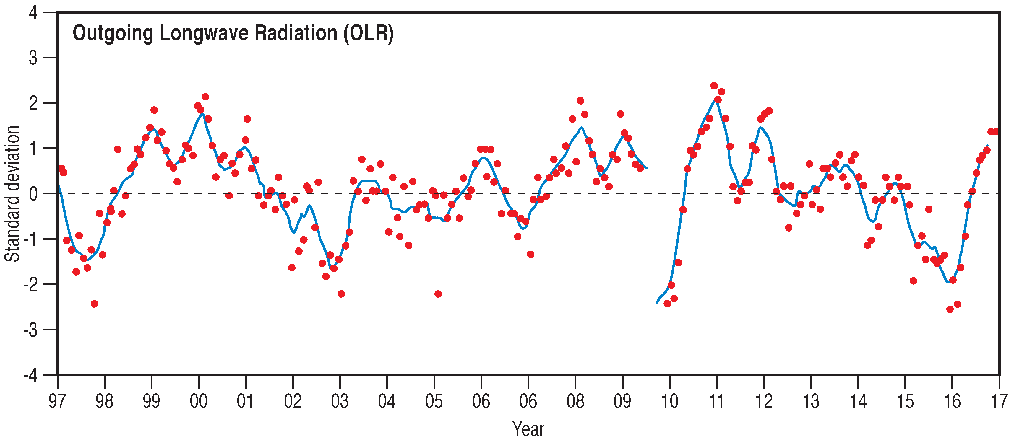
Figure 4.
Time series of ENSO wind indices for various regions (see Table 2) 1997–2016. The weakening of the zonal winds is especially apparent for the 1997–1998 El Niño event. Sourced and redrawn from the Climate Diagnostics Bulletin http://www.cpc.ncep.noaa.gov/products/CDB.
Figure 4.
Time series of ENSO wind indices for various regions (see Table 2) 1997–2016. The weakening of the zonal winds is especially apparent for the 1997–1998 El Niño event. Sourced and redrawn from the Climate Diagnostics Bulletin http://www.cpc.ncep.noaa.gov/products/CDB.

Figure 5.
Niño sea surface temperature regions (see Table 2). Sourced and redrawn from Barnston [21] https://www.climate.gov/news-features/blogs/enso/why-are-there-so-many-enso-indexes-instead-just-one.
Figure 5.
Niño sea surface temperature regions (see Table 2). Sourced and redrawn from Barnston [21] https://www.climate.gov/news-features/blogs/enso/why-are-there-so-many-enso-indexes-instead-just-one.

Figure 6.
Time series of SST anomalies (°C) for NIÑO regions (see Table 2 and Figure 5) 1997–2016. The strong positive SST anomalies are especially apparent for the 1997–1998 and 2015–2016 El Niño events. Notice also how the SST anomalies generally decrease in magnitude to the west. Sourced and redrawn from the Climate Diagnostics Bulletin http://www.cpc.ncep.noaa.gov/products/CDB.

Figure 7.
Canonical climate impact patterns of El Niño for (a) December–February and (b) June–August. Sourced and redrawn from the Climate Predicition Centre http://www.cpc.ncep.noaa.gov/products/analysis_monitoring/ensostuff/ensofaq.shtml#GLOBALimpacts.
Figure 7.
Canonical climate impact patterns of El Niño for (a) December–February and (b) June–August. Sourced and redrawn from the Climate Predicition Centre http://www.cpc.ncep.noaa.gov/products/analysis_monitoring/ensostuff/ensofaq.shtml#GLOBALimpacts.

Figure 8.
Canonical climate impact patterns of La Niña for (a) December–February and (b) June–August. Sourced and redrawn from the Climate Predicition Centre http://www.cpc.ncep.noaa.gov/products/analysis_monitoring/ensostuff/ensofaq.shtml#GLOBALimpacts.
Figure 8.
Canonical climate impact patterns of La Niña for (a) December–February and (b) June–August. Sourced and redrawn from the Climate Predicition Centre http://www.cpc.ncep.noaa.gov/products/analysis_monitoring/ensostuff/ensofaq.shtml#GLOBALimpacts.

Figure 9.
Rainfall anomalies for (a) El Niño and (b) El Niño Modoki events. Sourced and redrawn from Japan Agency for Marine, Earth Science and Technology. http://www.jamstec.go.jp/frcgc/research/d1/iod/enmodoki_home_s.html.en.
Figure 9.
Rainfall anomalies for (a) El Niño and (b) El Niño Modoki events. Sourced and redrawn from Japan Agency for Marine, Earth Science and Technology. http://www.jamstec.go.jp/frcgc/research/d1/iod/enmodoki_home_s.html.en.


Figure 10.
Range of El Niño related health impacts. Sourced and redrawn from the World Health Organisation. http://www.who.int/hac/crises/el nino/who_el_nino_and_health_global_report_21jan2016.pdf.
Figure 10.
Range of El Niño related health impacts. Sourced and redrawn from the World Health Organisation. http://www.who.int/hac/crises/el nino/who_el_nino_and_health_global_report_21jan2016.pdf.


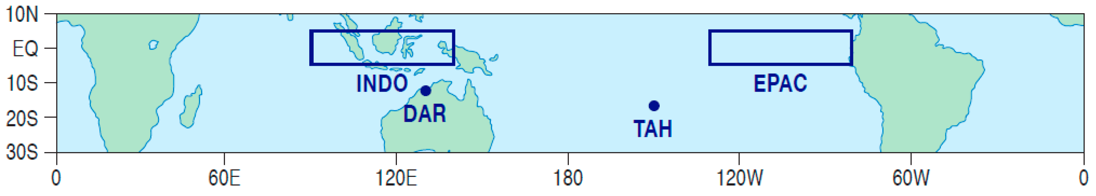
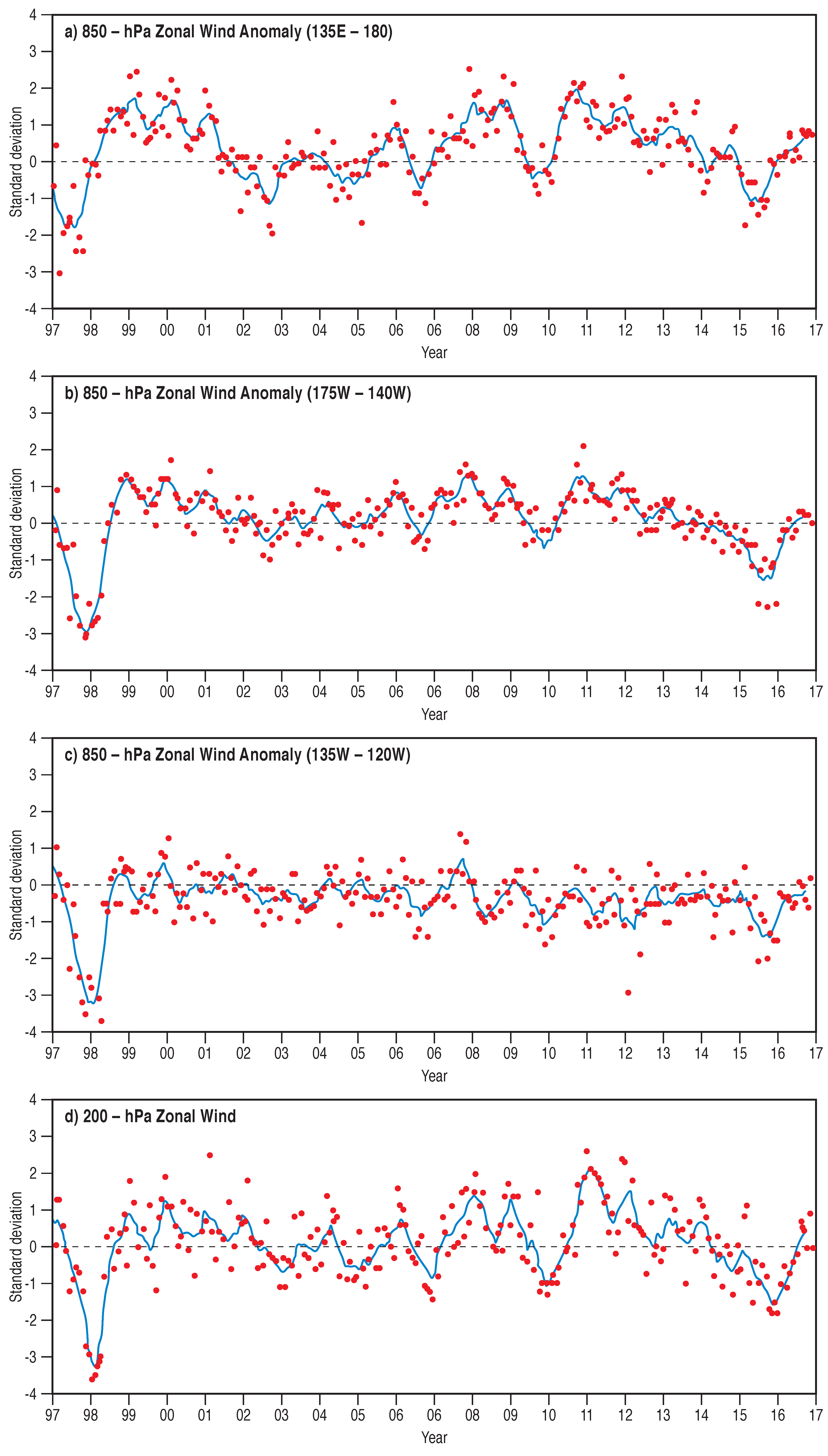
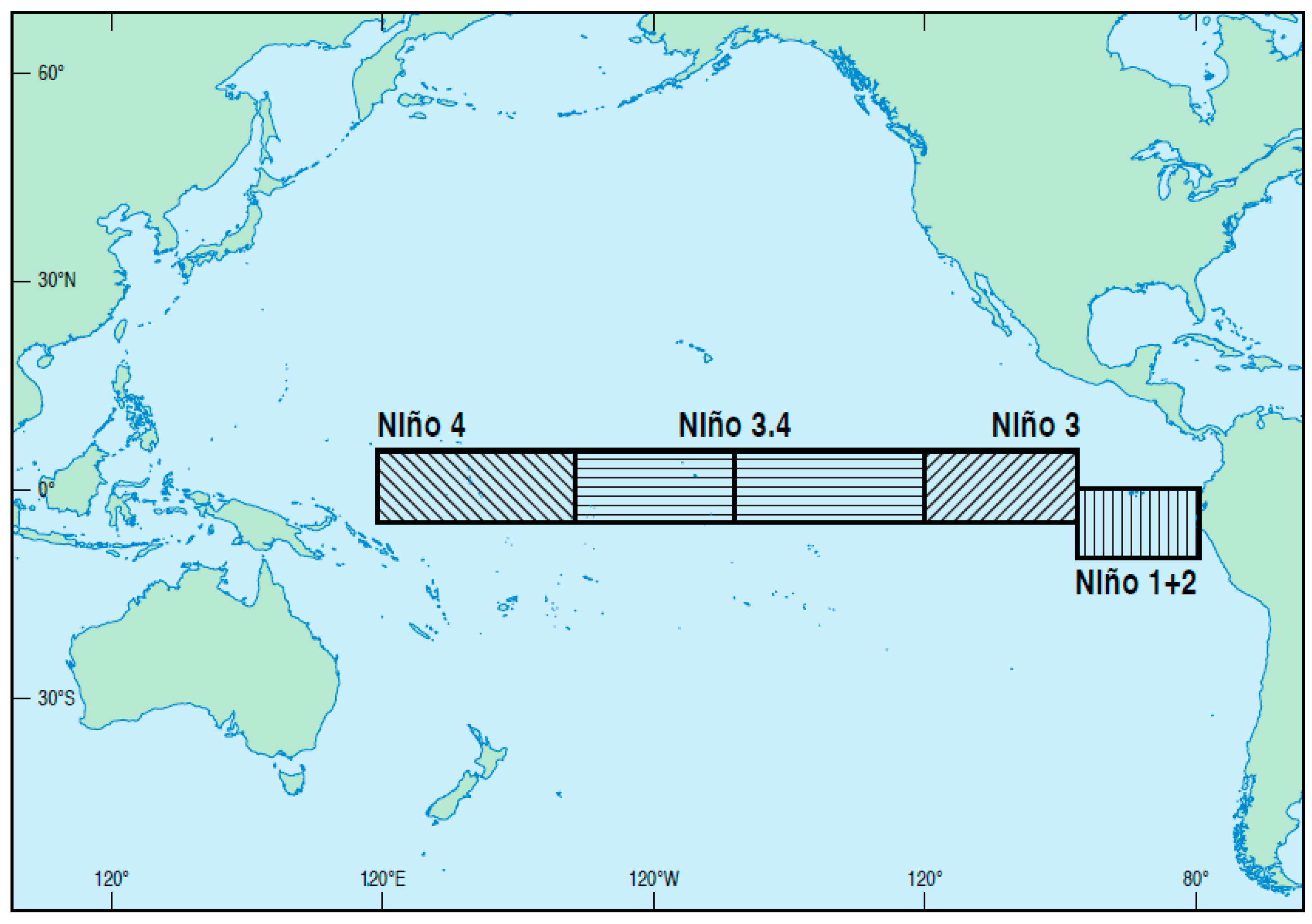
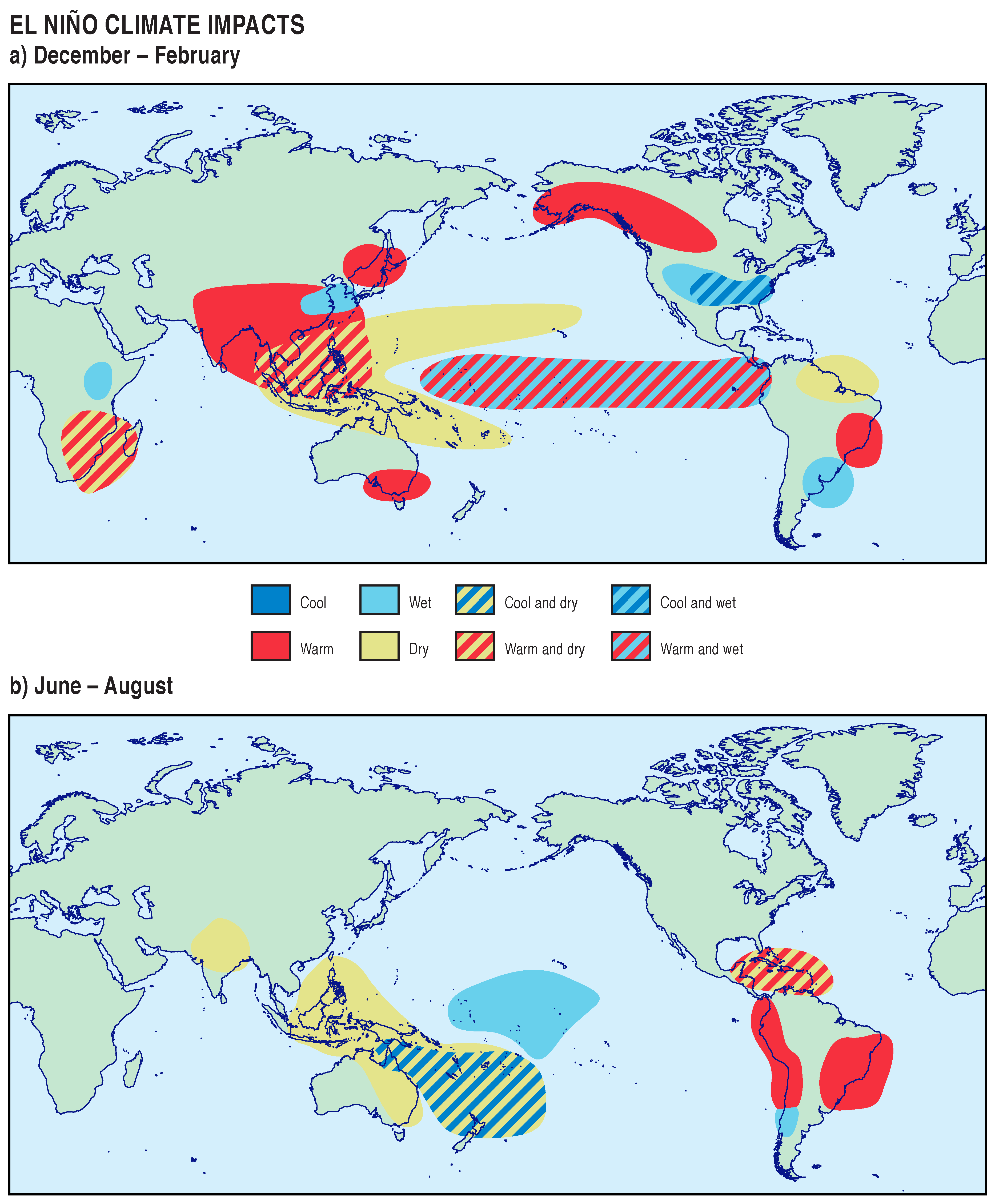
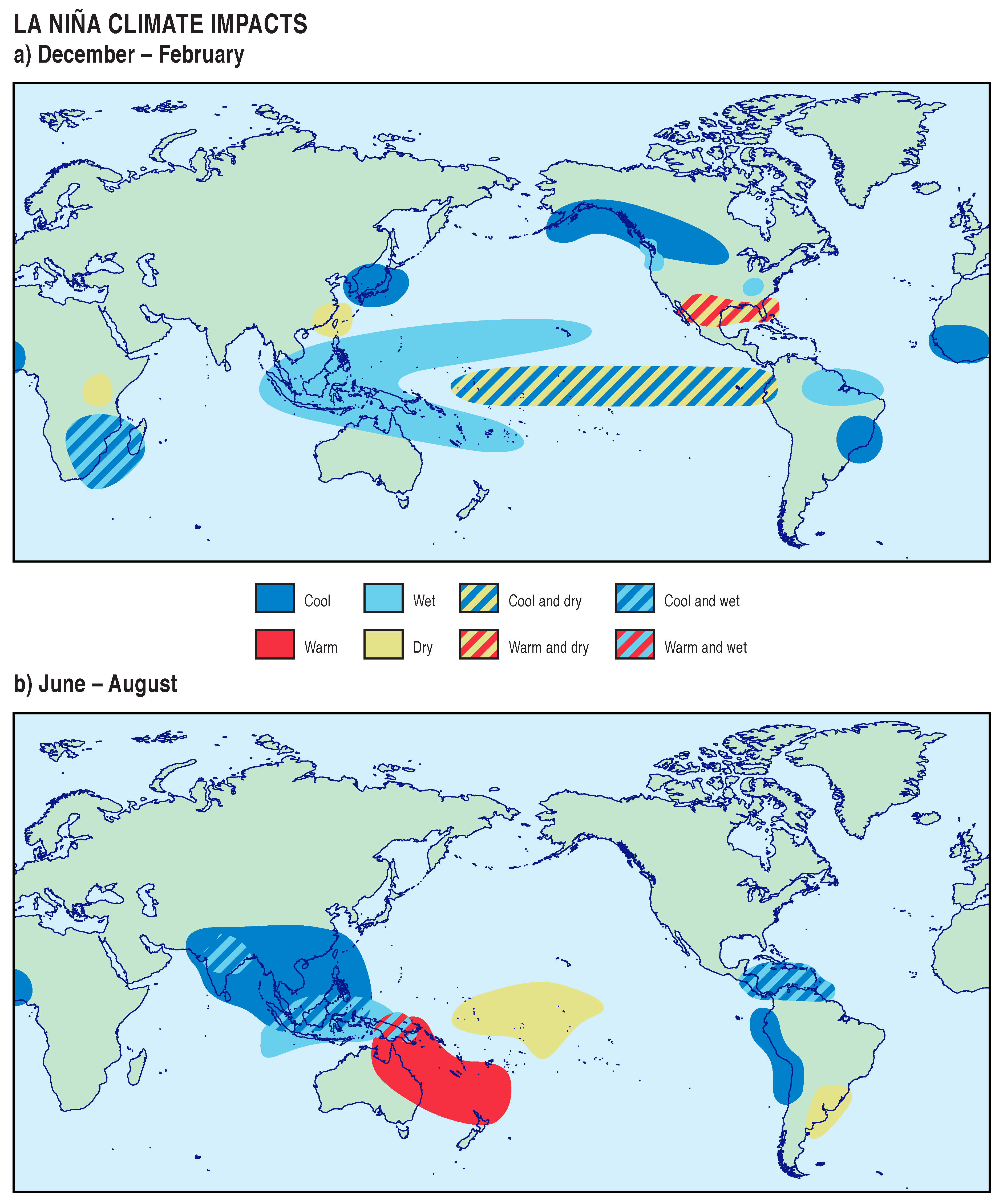
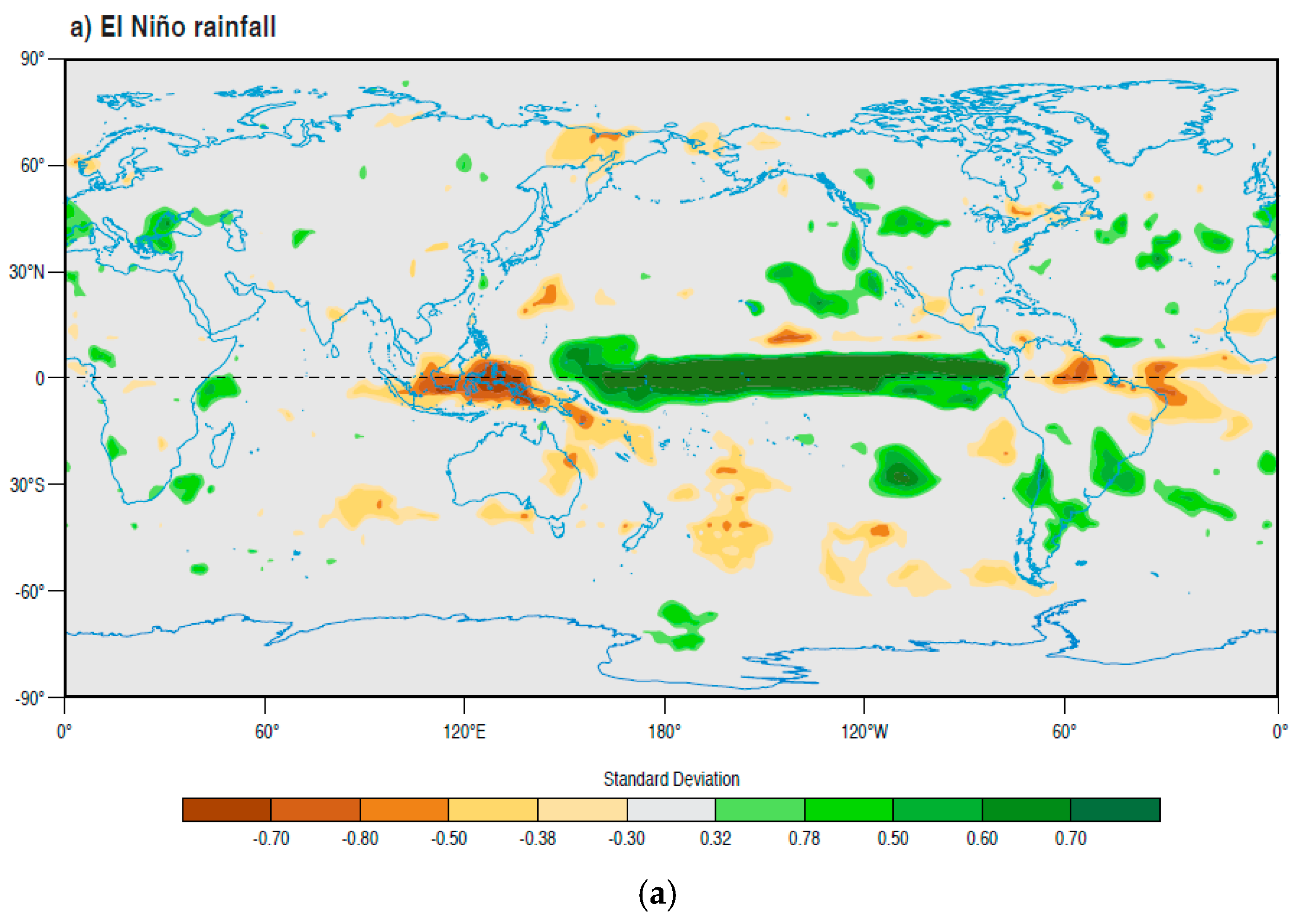
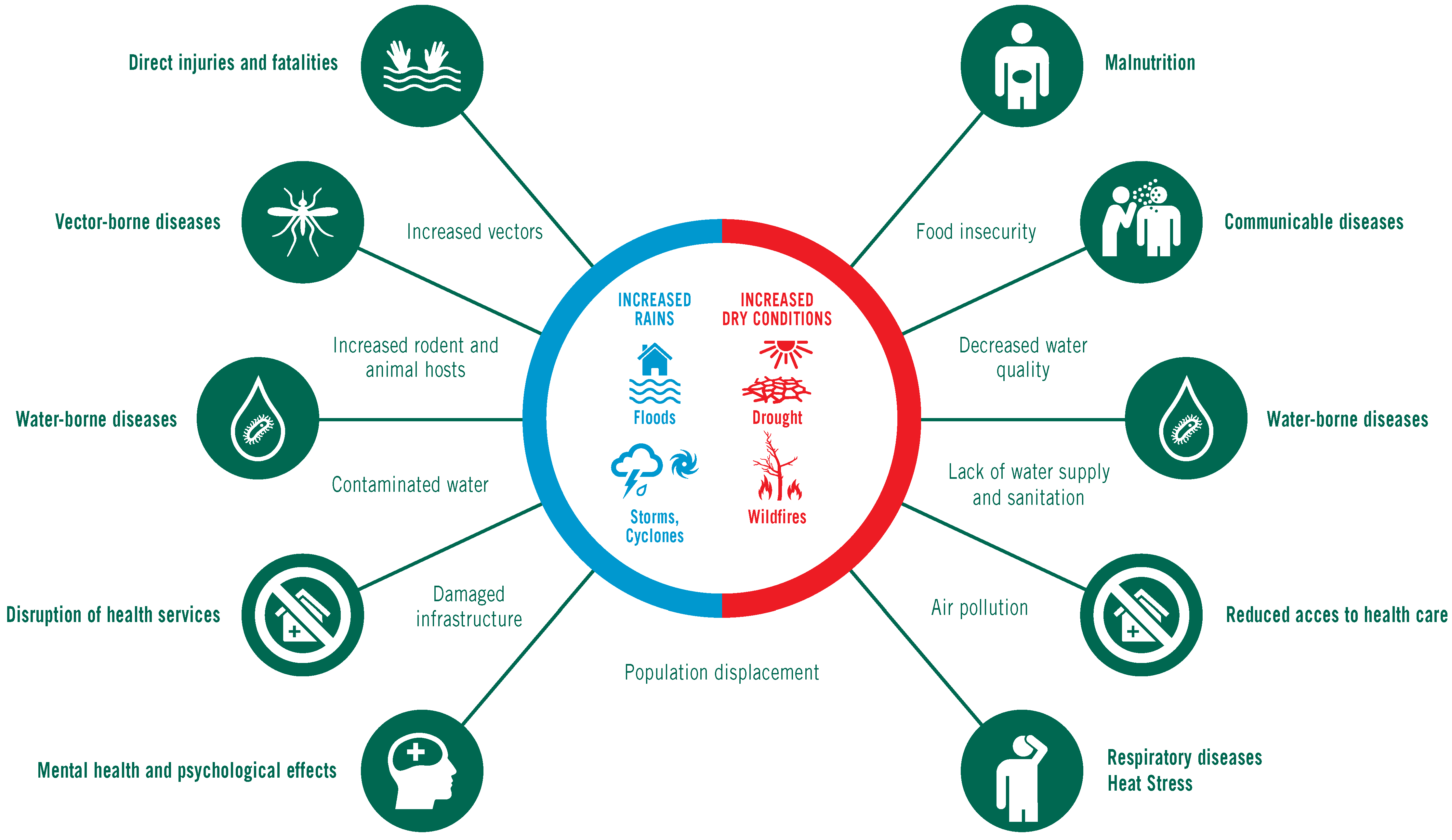
Table 1.
A selection of teleconnection patterns and indices (Source: McGregor [6]).
Table 1.
A selection of teleconnection patterns and indices (Source: McGregor [6]).
| Arctic Oscillation (AO)/Northern Annual Mode (NAM) | El Niño Southern Oscillation (ENSO) |
|---|---|
| North Atlantic Oscillation (NAO) | East Atlantic Pattern (EA) |
| West Pacific Pattern (WP) | East Pacific/North Pacific Pattern (EP/NP) |
| Pacific/North American Pattern (PNA) | East Atlantic/West Russia Pattern (EA/WR) |
| Scandinavia Pattern (SCA) | Northern Hemisphere Pattern (TNH) |
| Polar/Eurasia Pattern (POL) | Pacific Transition Pattern (PT) |
| Pacific South American Pattern (PSA) | Southern Annular Mode (SAM)/Antarctic Oscillation (AO) |
| Indian Ocean Dipole (IOD) | South Pacific Wave Pattern (SPW) |
| Quasi Biennial Oscillation (QBO) | Madden Julian Oscillation (MJO) |
| Pacific Decadal Oscillation (PDO) | Atlantic Meridional Oscillation (AMO) |
Table 2.
El Niño Southern Oscillation (ENSO) indices commonly reported by NOAA on a monthly basis. Modified from the Climate Diagnostics Bulletin http://www.cpc.ncep.noaa.gov/products/CDB.
Table 2.
El Niño Southern Oscillation (ENSO) indices commonly reported by NOAA on a monthly basis. Modified from the Climate Diagnostics Bulletin http://www.cpc.ncep.noaa.gov/products/CDB.
| Index | Index Name | Variable | Form of Index Value | Region (in Degrees) |
|---|---|---|---|---|
| Type | ||||
| Atmospheric | ||||
| Southern Oscillation Index (SOI) | Pressure | Standardised pressure difference between Tahiti and Darwin | Uses the single location of Darwin and Tahiti | |
| 850-hPa Trade Wind Index 1 | Wind direction and speed, Southwest Pacific | Standardised by mean annual standard deviation for reference period 2 | 5 N–5 S 135 E–180 | |
| 850-hPa Trade Wind Index 1 | Wind direction and speed, South Central Pacific | Standardised by mean annual standard deviation for reference period | 5 N–5 S 175 W–140 W | |
| 850-hPa Trade Wind Index 1 | Wind direction and speed, Southeast Pacific | Standardised by mean annual standard deviation for reference period | 5 N–5 S 135 W–120 W | |
| 200-hPa Zonal Wind Index 3 | Wind direction and speed, Central to Eastern Equatorial Pacific | Standardised by mean annual standard deviation for reference period | 5 N–5 S 165 W–110 W | |
| Outgoing Longwave Radiation Index (OLR) 4 | Longwave radiation in W/m 2 | Standardised by mean annual standard deviation for reference period | 5 N–5 S 160 E–160 W | |
| Oceanic | ||||
| NIÑO 1 + 2 | Pacific sea surface temperature (SST) in °C | Departures from 1981–2010 mean | 0–10 S 90 W–80 W | |
| NIÑO 3 | Pacific SST in °C | Departures from 1981–2010 mean | 5 N–5 S 150 W–90 W | |
| NIÑO 3.4 | Pacific SST in °C | Departures from 1981–2010 mean | 5 N–5 S 170 W–120 W | |
| NIÑO 4 | Pacific SST in °C | Departures from 1981–2010 mean | 5 N–5 S 160 E–150 W | |
| North Atlantic | Atlantic SST in °C | Departures from 1981–2010 mean | 5 N–20 N 60 W–30 W | |
| South Atlantic | Atlantic SST in °C | Departures from 1981–2010 mean | 0–20 S 30 W–10 E | |
| Global tropics | Global Tropics SST in °C | Departures from 1981–2010 mean | 10 N–10 S 0 W–360 W |
1 Positive (negative) values of 850-hPa zonal wind indices imply easterly (westerly) anomalies. 2 Currently NOAA uses 1981–2010 as the base period. 3 Positive (negative) values of 200-hPa zonal wind index imply westerly (easterly) anomalies. 4 Positive (negative) values indicate large amounts of outgoing longwave radiation.
Table 3.
Years in which strong and weak ENSO phases developed (Source: Santoso et al. [48]).
Table 3.
Years in which strong and weak ENSO phases developed (Source: Santoso et al. [48]).
| Strong El Niño | 1957, 1965, 1972, 1982, 1991, 1997, 2009, 2015 |
| Weak El Niño | 1963, 1968, 1976, 1977, 1987, 1994, 2002, 2006 |
| Strong La Niña | 1973, 1975, 1988, 1998, 1999, 2007, 2010 |
| Weak La Niña | 1950, 1954, 1955, 1964, 1970, 1971, 1984, 1995, 2000, 2005, 2008, 2011 |
| Central Pacific (CP) El Niño | 1958, 1968, 1977, 1979, 1987, 1990, 1994, 2002, 2004, 2006, 2009, 2014 |
© 2018 by the authors. Licensee MDPI, Basel, Switzerland. This article is an open access article distributed under the terms and conditions of the Creative Commons Attribution (CC BY) license (http://creativecommons.org/licenses/by/4.0/).
Share and Cite
MDPI and ACS Style
McGregor, G.R.; Ebi, K. El Niño Southern Oscillation (ENSO) and Health: An Overview for Climate and Health Researchers. Atmosphere 2018, 9, 282. https://doi.org/10.3390/atmos9070282
AMA Style
McGregor GR, Ebi K. El Niño Southern Oscillation (ENSO) and Health: An Overview for Climate and Health Researchers. Atmosphere. 2018; 9(7):282. https://doi.org/10.3390/atmos9070282
Chicago/Turabian StyleMcGregor, Glenn R., and Kristie Ebi. 2018. "El Niño Southern Oscillation (ENSO) and Health: An Overview for Climate and Health Researchers" Atmosphere 9, no. 7: 282. https://doi.org/10.3390/atmos9070282
Note that from the first issue of 2016, this journal uses article numbers instead of page numbers. See further details here.