A Velocity Dealiasing Algorithm on Frequency Diversity Pulse-Pair for Future Geostationary Spaceborne Doppler Weather Radar


1
College of Electronic Engineering, Chengdu University of Information Technology, Chengdu 610225, China
2
China Meteorological Administration, Key Laboratory of Atmospheric Sounding, Chengdu 610225, China
3
Meteorological Information and Technology Center, Chongqing Meteorological Bureau, Chongqing 401147, China
*
Author to whom correspondence should be addressed.
Atmosphere 2018, 9(6), 234; https://doi.org/10.3390/atmos9060234
Submission received: 29 April 2018
/
Revised: 8 June 2018
/
Accepted: 14 June 2018
/
Published: 15 June 2018
(This article belongs to the Special Issue Radar and Satellite Observations of Precipitation Systems: Climate Applications)
Abstract
:Velocity ambiguity is one of the main challenges in accurately measuring velocity for the future Geostationary Spaceborne Doppler Weather Radar (GSDWR) due to its short wavelength. The aim of this work was to provide a novel velocity dealiasing method for frequency diversity for the future implementation of GSDWR. Two different carrier frequencies were transmitted on the adjacent pulse-pair and the order of the pulse-pair was exchanged during the transmission of the next pulse-pair. The Doppler phase shift between these two adjacent pulses was estimated based on the technique of the frequency diversity pulse-pair (FDPP), and Doppler velocity was estimated on the sum of the Doppler phase within the adjacent pulse repetition time (PRT). From the theoretical result, the maximum unambiguous velocity estimated by FDPP is only decided by the interval time of the two adjacent pulses and radar wavelength. An echo signal model on frequency diversity was established to simulate echo signals of the GSDWR to verify the extension of the maximum unambiguous velocity and the accuracy of the velocity estimation for FDPP used on GSDWR. The study demonstrates that the FDPP algorithm can extend the maximum unambiguous velocity greater than the Stagger PRT method and the unambiguous range and velocity are no longer limited by the chosen value of pulse repetition frequency (PRF). In the Ka band, the maximum unambiguous velocity can be extended to 105 m/s when the interval time is 10 μs and most velocity estimation biases are less than 0.5 m/s.
1. Introduction
Space-borne Precipitation Radar (SPR) is an active measurement radar used on a satellite platform that can observe rainfall characteristics in all weather conditions at all times with three-dimensional (3D) detection in the range of the radar observation. SPR is the only effective tool that directly obtains global rainfall information [1]. The development of the SPR began in the 1980s. The first SPR was carried on the Tropical Rainfall Measuring Mission satellite, which was launched in 1997 [2]. The Dual Frequency Precipitation Radar (DPR) is working, carried by the Global Precipitation Measurement (GPM) that was launched in 2013 [3]. While studying the low-orbiting SPR, National Aeronautics and Space Administration (NASA) proposed the Next-Generation Radar (NEXRAD) in the space research project to deploy a weather radar in geostationary orbit for hurricane detection. In contrast to low-orbiting SPR, the Geostationary Spaceborne Doppler Weather Radar (GSDWR) not only provides high-frequency, wide-coverage rainfall detection, but also typhoon and strong storm monitoring near 1 h or higher frequencies. In addition, GSDWR not only measures precipitation fall speed, but also the movement of the horizontal wind field.
However, the GSDWR project faces many new challenges in the measurement of Doppler velocity, such as Doppler velocity ambiguity. Since the maximum unambiguous velocity of the short wavelength (Ka band) is relatively small, velocity ambiguity often occurs when measuring the speed of strong storms and hurricanes and other severe weather, which seriously affects the accuracy of the velocity measurement and causes large estimation error in the echo spectral moment estimation. The detection of strong storms and hurricanes is one of the main purposes of GSDWR. Therefore, we focused on the velocity ambiguity problem and created a method for velocity dealiasing for GSDWR to improve the efficiency, which is extraordinarily significant for GSDWR.
The most commonly used methods of velocity dealiasing include the staggered pulse repetition time (PRT) algorithm, dual pulse repetition frequency (PRF), batch processing, and polarization diversity pulse-pair (PDPP). The stagger PRT method was introduced by Sirmans to be used in a weather radar in 1976 [4,5], but because of non-uniform sampling, the signal and clutter spectrum change [6], so the use of this method has been limited for a long time. Of course, there is more research on dual PRF technology in recent years [7]. In 1997, Sachidananda and Zrnic put forward a method for solving distance ambiguity using the phase encoding of a SZ system [8]. This algorithm was validated by the National Center for Atmospheric Research (NCAR) and National Severe Storms Laboratory (NSSL). In 2006, Zhou [9] introduced batch processing to solve the weather radar data ambiguity problem and this method was able to separate overlapping echoes from time. In 1998, Pazmany proposed polarization diversity pulse-pair (PDPP) [10,11], which can effectively solve Doppler ambiguity but is only suitable for a dual polarization radar. However, each method has some disadvantages that require improvement. In this paper, we introduce a novel method for frequency diversity pulse-pair to extend the maximum unambiguous velocity while maintaining the accuracy of velocity estimation. The aim of this study was to provide a velocity dealiasing method for future GSDWR.
In this paper, the velocity ambiguity problem faced by GSDWR is firstly analyzed according to the relationship between satellite geometry and radial velocity measurement for hurricane observation. Then, a velocity dealiasing algorithm for frequency diversity pulse-pair (FDPP) is introduced and analyzed, which changes the interval time of the adjacent transmitting pulses to obtain better performance in the extension of the maximum unambiguous velocity and the velocity estimation accuracy. To evaluate the performance of FDPP used in GSDWR, a GSDWR echo model of frequency diversity is then built and simulated. The results show that this FDPP algorithm has better velocity estimation performance and can extend the maximum unambiguous velocity for GSDWR. Although the study is focused on spaceborne techniques, it can be also of interest to researchers working on improved Doppler radar velocity estimates, such as wind shear and mesocyclone storm detection [12].
2. GSDWR System and Velocity Ambiguity Analysis
2.1. GSDWR Introduction
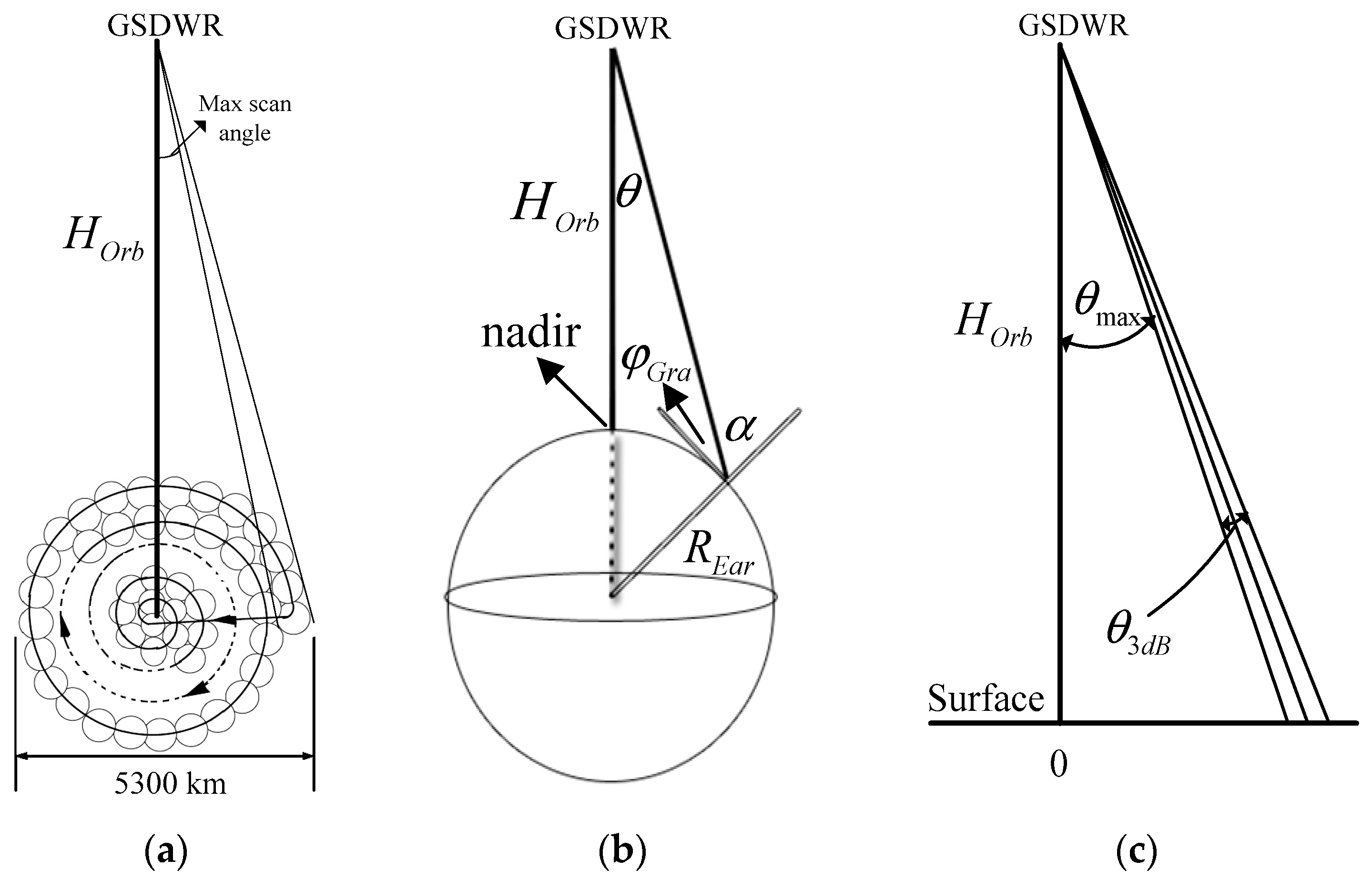
Although the Geostationary Spaceborne Doppler Weather Radar (GSDWR) is still a conceptual radar [1,13,14], it has been studied in the United States and China and some of the related parameters of the radar system are shown in Table 1. The GSDWR is designed to work in geostationary orbit at an altitude of 36,000 km, with a maximum scan angle of 4°, and a spiral scanned antenna beam [15]. The scan model is shown in Figure 1a.
The geometric relationship between the satellites and the earth is shown in Figure 1b, which can be expressed with Equations (1) and (2). The orbit height HOrb is 36,000 km, radar beam scan angle θ ranges from 0° to 4°, and the earth radius REar is 6370 km.
where is the grazing angle. When the beam scan angle θ = 4°, = 62.36° and the incident angle α = 27.64°.
For the Doppler weather radar, the choice of PRF is crucial. Distance ambiguity cannot occur in the range of attention. It is necessary to consider the pulse generation, transmission time tolerance, and the switching time between the transmitting and receiving states. The correlation and independence between the echo signal samples and the Nyquist sampling rate also must be considered [16]. According to Figure 1c and Equation (3), where c is the speed of light, when the maximum detection distance H is 25 km and the scan angle range θ is 0° to 4°, the maximum PRF is 6 kHz.
2.2. Velocity Ambiguity of GSDWR
For the Geostationary satellite platform, we assumed that the speed of the satellite platform motion has no effect on the Doppler radial velocity component of GSDWR, so the Doppler radial velocity component observed by GSDWR can be computed as follows [13]:
where u, v, and w are the velocity components of the 3D wind field, vT is the terminal velocity of the precipitation, and the angle θ and γ represent the incident angles of the beam in the east–west direction and the north–south direction, respectively, which can be expressed by Equation (5) [13].
where α and β represent the pointing angles in the north–south and the east–west direction, respectively; d is the distance between radar and meteorological target; and a is the earth’s radius. For simple evaluation of the relationship of radar radial velocity component with the horizontal wind field, we focused on the radial velocity component vrad from the composed horizontal wind speed VH from (u, v). From Equations (4) and (5), VH can be obtained by:
The problems facing the Doppler weather radar include maximum unambiguous range and maximum unambiguous velocity, and these two values are both determined by the value of the PRF [17,18]. The two values, respectively, are expressed by:
where c is the velocity of light and λ is the radar wavelength. Usually, in the spaceborne Doppler weather radar design, we firstly attempted to choose the correct PRF value to ensure there is no range ambiguity. To demonstrate the velocity ambiguity problem, a maximum range of 25 km for the range of precipitation observation was assumed. According to Equation (8), the PRF value could not be larger than 6 kHz; therefore, the maximum unambiguous velocity was 12.7 m/s. Taking the Saffir–Simpson Hurricane Wind Scale (SSHS) [19] as an example, the maximum horizontal wind speed is 59–69 m/s at SSHS-4 and ≥70 m/s at SSHS-5. Given the SSHS-5 horizontal velocity was 70 m/s, according to Equation (6), the relationship between the pointing angles (α and β) and the maximum radial velocity vrad can be obtained, as shown in Figure 2.
From Figure 2, when SSHS-5 is observed by GSDWR, the radial velocity in the areas of pointing angles from 2° to 4° or −2° to −4° will be larger than the maximum unambiguous velocity of 12.7 m/s. If we added the terminal and vertical velocity components into the result of the radar radial velocity component, the area of the pointing angles will be further expanded and the problem of velocity ambiguity will become worse. As one of the main advantages of GSDWR is that it can observe and trace hurricanes and typhoons more frequently with its stationary observation of the earth, if the problem of velocity ambiguity cannot be resolved, the whole application of GSDWR will be affected.
3. Frequency Diversity Pulse-Pair Algorithm
3.1. FDPP Algorithm Principle
The Frequency Diversity Pulse-Pair (FDPP) algorithm is an improvement based on the stagger PRT algorithm [20,21]. Two pulses with different center frequencies of f1 and f2 are transmitted with a separation ΔT during the first PRT, and an inverting order pulse is transmitted with a separation ΔT during the next PRT. The pulse transmission mode of the FDPP algorithm is shown in Figure 3. Two central frequencies of f1 and f2 are in the pulse that is transmitted with an interval ΔT, but after time T, the order of the pulses is reversed and transmitted (Figure 3).
In the receiver, the pulse-pair phase estimates of f1−f2 and f2−f1 are individually accumulated and recorded as ΔΦR1 and ΔΦR2, respectively. Then, the Doppler velocity vr is estimated from the sum of ΔΦR1 and ΔΦR2. The detailed deduction of vr is shown in Appendix A.
Because the sum of ΔΦR1 and ΔΦR2 is between [−π, π], the maximum unambiguous velocity expression is as shown in Equation (10).
The FDPP algorithm velocity estimate is same as the conventional pulse-pair algorithm by calculating the phase information through the correlation function. According to the correlation function previously defined [4], the variance in calculating ΔΦR1 and ΔΦR2 is same and can be expressed with Equation (11).
The spectrum width σv can be expressed as:
3.2. Analysis of FDPP Algorithm
In this section, the FDPP algorithm performance is theoretically analyzed with the algorithm above. In the calculation, f1 = 35.5 GHz, f2 = f1 + 10 MHz, ΔT = 10 μs, the theoretical maximum unambiguous velocity under these conditions is 105.5 m/s. Figure 4a shows the phase results of ΔΦR1 and ΔΦR2. From the figure, the phase directly calculated from Equation (9) appears folded and it limits the range of the maximum unambiguous velocity. If the phase is now directly used in Equation (9), the velocity value will not be as great as the theoretical maximum unambiguous velocity. We propose a phase modification method as shown in Equation (13), where k represents the number of phase folds, and here, k = 1. The velocity comparison between phase modification and no modification is shown in Figure 4c.
From analysing Equation (10), the maximum unambiguous velocity of FDPP is only related to ΔT and wavelength, which are independent of the PRF and completely solves the Doppler problem. However, the choice of PRF has a certain relationship with the accuracy of the velocity estimation. In addition, the accuracy of velocity estimation is influenced by the signal to noise ratio (SNR) and ΔT. When ΔT = 10 μs and the pulse width is 10 μs, the pulse central frequency f1 is 35.5 GHz, and f2 = f1 + 10 MHz. The relationship between the velocity estimation error and SNR is shown in Figure 5a. When the SNR is greater than −6 dB, the velocity estimation error is small, but when the SNR is less than −6 dB, the velocity estimation error increases with the decrease in the SNR. Similarly, Figure 5b shows the trend in the velocity estimation error with different SNR. When PRF is less than 9 kHz, the velocity estimation error is relatively small, and when the SNR is smaller, the estimation error is greater. Equation (10) shows that ΔT determines the maximum unambiguous velocity, but it is not as small as possible due to the accuracy of the velocity estimation. Using the same conditions above, at PRF = 4000 Hz, the velocity estimation error is evaluated with different ΔT, and the results are shown in Figure 5c. From the results, when ΔT is larger than 5 μs, the velocity estimation errors are small and the needs of GSDWR, whose pulse width will be 5–50 μs, can be met.
4. Simulation and Results Discussion
4.1. Echo Simulation of GSDWR
Due to the limited conditions, GSDWR could not verify the algorithm or the whole machine performance through real experimental data. Related research used airborne radar or ground-based radar data to simulate space-borne weather radar echo signals [22]. The Earth Clouds, Aerosols, and Radiation Explorer (Earth CARE) satellite carried a spaceborne 94-GHz Doppler Cloud Profiling Radar (CPR), which included a synthetic echo signal from ground-based radar data, was used for algorithm validation and performance evaluation [23]. However, the echo signal simulation from the power spectrum, and generating frequency diversity time series from the spectrum, were not feasible in this paper. Therefore, the time domain echo signal model was used to simulate the GSDWR echo signal in this article. However, attenuation and weighting and other factors must also be considered. Firstly, the spatial distribution of the precipitation particles model was established by the rectangular grid method shown as Figure 6a, which ignored the influence of the curvature of the earth. The precipitation space was divided into several precipitation cells and all the particles in the precipitation cell were treated as a scattering unit. These precipitation particles had a certain relative motion [24]. According to the measured APR-2 data and Figure 6a, the spatial precipitation distribution model was established and the Gaussian distributed pseudo-random values were used to generate the particle relative velocity field in the precipitation cell [21]. The echo of the precipitation cell was calculated by the echo signal model as shown in Equation (14), and the precipitation particle relative parameters were determined, including position, velocity, antenna gain, and the path integral attenuation. The echo signal deduction model is shown in Appendix B.
where f0 is carrier frequency, u(t) is the complex envelope function of the signal, τi is the echo delay of the ith precipitation cell, which is determined by the radial distance and relative velocity of the precipitation target cell and radar, fd is the Doppler shift, and N is the number of the precipitation cell.
However, the resolutions of APR-2 data and GSDWR data are different; a GSDWR data cell consists of 30 × 8 APR-2 data. Therefore, the antenna gain corresponding to the precipitation particles is different in different positions in a GSDWR beam element, so that the echo power is also different and must, therefore, be antenna weighted [25]. The weighting function expression is shown in Equation (15). To improve the detection ability of the spaceborne radar, the advanced pulse compression technology was used to improve the distance resolution, so the distance weighting was used. The distance weighting function uses the ambiguous function of the transmitting signal, as shown in Equation (17). The antenna weighted and distance weighted schemes are shown in Figure 6b.
where
4.2. Analysis of the Simulation Results
The GSDWR simulations were obtained using the environmental field data measured by the Ka-band of the APR-2 weather radar. The APR-2 data were considered to eliminate factors such as aircraft attitude and jitter that may affect data quality. Firstly, according to the GSDWR parameters, FDPP model, and Equation (14), the APR-2 data of reflectivity and Doppler radial velocity were used to generate the echo signal. Then, the FFT transform was performed for the echo signal and the power spectrum was obtained. The GSDWR power spectrum was obtained by range and antenna weighting, and then the I/Q serial was obtained by inverse Fourier transform of the weighted power spectrum. Finally, the FDPP algorithm was used to estimate velocity and width. The flowchart of the simulation is shown in Figure 7a. The APR-2 echo reflectivity and velocity data are shown in Figure 7b. To quantitatively verify the velocity dealiasing effectiveness of the FDPP algorithm for GSDWR, the 30 (horizontal) × 216 (vertical) APR-2 data was used to constitute the radial data of GSDWR, as shown by the data range drawn in the red rectangle A as shown in Figure 7b.
Rectangle data A was used to simulate the GSDWR echo signal in FDPP mode, and the parameters were set as: PRF = 4000 Hz, f1 = 35.5 GHz, f2 = 35.51 GHz, ΔT = 10 μs, and SNR = 10 dB. When using the PPP algorithm to estimate velocity, the maximum unambiguous velocity was 8.5 m/s. For the FDPP algorithm, the maximum unambiguous velocity was 105.6 m/s. The results of the radial velocity estimation are shown in Figure 8a, which shows that when the virtual velocity is greater than 8 m/s in the range of one to three kilometers, the velocity of the PPP estimation has folded, but the velocity of the FDPP estimation can accurately estimate the velocity value.
To verify that the selection of PRF in the FDPP algorithm has no direct effect on the maximum unambiguity velocity, the PRF was adjusted to satisfy the maximum unambiguity distance. We adjusted the PRF to 1000 Hz, resulting in a maximum unambiguous velocity with PPP estimation algorithm of 2.1 m/s, and a maximum unambiguous velocity with FDPP estimation algorithm of 105.6 m/s. From Figure 8b, the velocity of the traditional PPP method always has ambiguous velocity, and then the FDPP estimation results are acceptable.
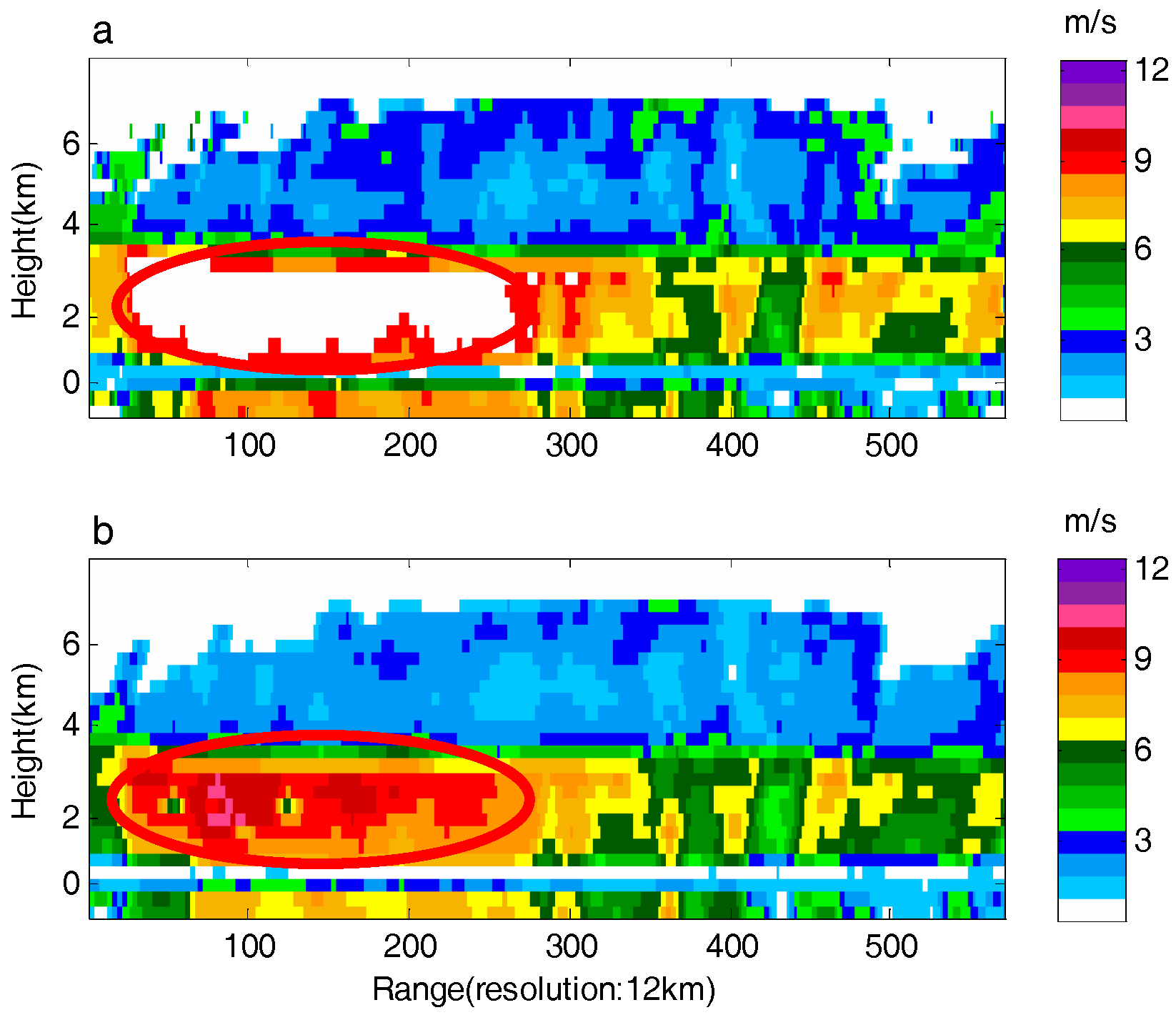
Figure 9 shows the GSDWR radial velocity echo data according to Figure 7b and the same simulation conditions above. The actual horizon resolution is very poor, so horizontal slide processing was used to obtain more horizontal data for a better effect. Figure 9a displays the results obtained with the PPP method and Figure 9b provides the FDPP method results. Figure 9a shows the velocity ambiguity in the elliptic region, which occurred because the real velocity is greater than the maximum unambiguous velocity using the PPP method. Figure 9b shows the velocity value was estimated accurately in the ellipse region.
4.3. Performance Analysis of FDPP
The above analysis shows that the FDPP algorithm has a good velocity dealiasing effect. However, in actual applications, the precision of the velocity estimation needs to be considered. In the meteorological radar observation business, the precision of velocity estimation must be less than 1 m/s, and the GSDWR is proposed to be less than 0.5 m/s. Therefore, the velocity estimation bias of the FDPP algorithm under different SNR, PRF, and ΔT conditions was analyzed.
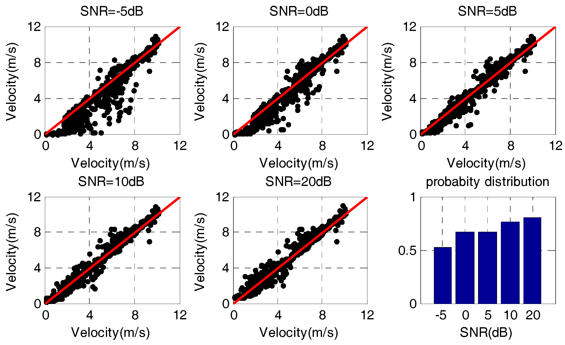
Figure 10 shows the velocity estimation scatter and statistic histogram, where the red line represents the zero-deviation standard in scatter, and the histogram indicates the probability of velocity bias being less than 0.5 m/s. From the scatter figure, with the increase in SNR, the more the velocity data focus on the zero-deviation standard line. The histogram shows that the velocity estimation precision improves with the increase in SNR, which is also consistent with the previous theoretical analysis.
Similarly, from the PRF analysis in Figure 11 and ΔT in Figure 12, almost no difference in velocity estimation accuracy was observed within the permitted range, which is also consistent with the previous theoretical analysis and Figure 5. Actually, when ΔT is 40 μs in Figure 11, the maximum unambiguous velocity is only about 26 m/s, and velocity ambiguity easily occurs for GSDWR.
To construct the velocity spectrum width information in this simulation, Gaussian random velocity distribution was constructed based on APR-2 velocity data with a maximum velocity change of 4 m/s. The velocity and velocity spectral width results using the FDPP algorithm when the SNR was 10 dB, PRF was 4000 Hz, and ΔT was 10 μs are shown in Figure 13a. The maximum spectral width was also 4 m/s.
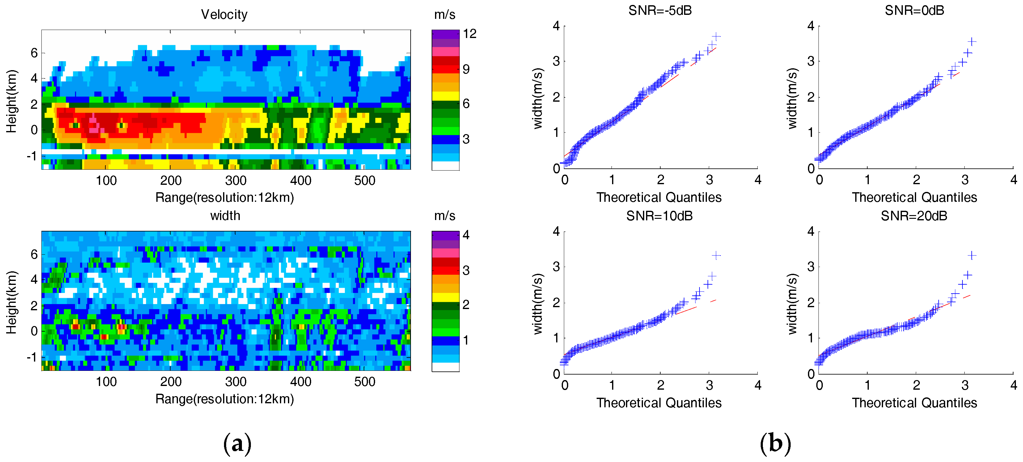
To further verify the validity of the velocity spectral width estimation, a QQPlot figure was used for verification analysis, as it can intuitively verify and analyze whether a group of data obeys or approaches a certain distribution characteristic. Figure 13b shows the distribution characteristics of the velocity spectrum width calculated under a variety of SNR conditions. Along with the increase in SNR, spectral width data were increasingly consistent with ideal distribution, which is also consistent with the spectral width distribution of the previous structure.
5. Conclusions
The Spaceborne Weather Radar is an effective tool for global precipitation observation. However, Doppler velocity ambiguity and range ambiguity are urgent problems. The frequency diversity pulse-pair method outlined in this paper can effectively solve the Doppler velocity and distance ambiguity problems, which are limited by the radar PRF and wavelength, especially for millimeter wave radar. We firstly analyzed the principle and performance of the FDPP algorithm. From the principle analysis, the maximum unambiguous velocity can be determined by the radar wavelength and the interval time ΔT of the adjacent pulse-pair. ΔT has a certain range of choices, rather than an unlimited or large range. Then, a GSDWR echo signal model was established, which verified the velocity dealiasing algorithm. According to the results analysis, we chose ΔT as 10 μs in Ka band, which extended the maximum unambiguous velocity to 105 m/s, but it was impossible through staggered PRT within appropriate values of PRF. Additionally, the velocity estimation precision was also fully considered. As with other velocity estimation methods, SNR had a relatively large effect on velocity estimation accuracy. When the SNR value was greater than 10 dB, most of the estimation error was less than 0.5 m/s. Simultaneously, the choice of ΔT and PRF value had little effect on the velocity estimation accuracy within the appropriate range. So, according to the maximum detection distance and velocity, we could dynamically choose these two parameters, ΔT and PRF, during deployment. Compared with staggered PRT, the FDPP introduced in this paper has a larger velocity extension range and estimation performance, providing a better solution for Doppler’s dilemma, especially for millimeter wave radar.
Author Contributions
C.W. and X.L. designed the experiments; C.W. performed the experiments and data analysis; Z.Q., F.L. and Q.S. designed the echo simulation; C.W. and X.L. analyzed the results; X.L. and J.H. supervised the work and provided comments on the results; C.W. wrote this paper.
Funding
This research received no external funding.
Acknowledgments
This work was supported by Natural Science Foundation of China (41575022, 41375043), Project of Sichuan Province (2014JY0093), Project of Chengdu University of Information Technology (KYTZ201414, J201601).
Conflicts of Interest
The authors declare no conflict of interest.
Appendix A
Assume that the transmission signals of the two pulses centered at f1 and f2 are Stf1 and Stf2, the expression is:
where ψf1 and ψf2 are the initial phase and ΔT is the diversity frequency pulse interval. Then, the meteorological target of velocity is vr at a distance of R1 km, and the echo signal received by the radar can be expressed as:
where Af1 and Af2 represent the scattering intensity of the pulse signal from the meteorological target. Assuming that Af1 = Af2 and Ef1 = Ef2, the phase difference between the echo signal and the transmitted signal are Φf1 and Φf2:
So, the phase difference between the f2 and f1 pulses is:
Similarly, if the target moves to R2 km at the next set of pulses, the difference between the f1 and f2 pulse is:
Then:
Because R2 = R1 + vT, k1 = 2πf1/c, and k2 = 2πf2/c, ΔΦ can be expressed as:
Approximately, we assume that k1 − k2 ≈ 0, k1 + k2 ≈ 2k1, and then:
So, the velocity can be expressed as:
Appendix B
Assuming that the transmitted signal is represented by st(t), the echo signal from the precipitation target is denoted by sr(t), and τt is the echo delay time. According the radar meteorological from Doviak and Zrnić [26], echo signal can expressed as formula (A10).
where G is antenna gain, θ and φ are the beam width in different directions, τ is the pulse width, λ is wavelength, As is the attenuation coefficient, and Z is reflectivity. Assuming that:
Normally, the transmitted radar signal is a narrowband signal and to achieve pulse compression, the signal is used as a linear frequency modulation signal. The complex expression of the signal st(t) is written as:
where f0 is the carrier frequency, u(t) is the complex envelope function and the expression is:
where Tm is the pulse width; k is the frequency modulation rake ratio, which is expressed as k = B/T; B is the bandwidth; and T is the pulse repetition period. The target echo signal of the precipitation particle at the ith point can be expressed as:
where τi is the echo delay of the ith precipitation cell, which is determined by the radial distance and relative velocity of the precipitation target cell and radar; fd is the Doppler shift; and N is the number of the precipitation cell. The amplitude of the echo signal is determined by the reflectivity, the corresponding antenna gain, and the path integral attenuation.
References
- Im, E.; Smith, E.A.; Durden, S.L.; Tanelli, S.; Huang, J.; Rahmat-Samii, Y.; Lou, M. Instrument concept of nexrad in space (NIS)—A geostationary radar for hurricane studies, Geoscience and Remote Sensing Symposium. In Proceedings of the 2003 IEEE International Geoscience and Remote Sensing Symposium, Toulouse, France, 21–25 July 2003; pp. 2146–2148. [Google Scholar]
- Kozu, T.; Kawanishi, T.; Kuroiwa, H.; Kojima, M.; Oikawa, K.; Kumagai, H.; Okamoto, K.I.; Okumura, M.; Nakatsuka, H.; Nishikawa, K. Development of precipitation radar onboard the tropical rainfall measuring mission (TRMM) satellite. IEEE Trans. Geosci. Remote Sens. 2001, 39, 102–116. [Google Scholar] [CrossRef]
- Tang, G.; Wan, W.; Zeng, Z.; Guo, X.; Li, N.; Long, D.; Hong, Y. An overview of the global precipitation measurement (GPM) mission and it’s latest development. Remote Sens. Technol. Appl. 2015, 30, 607–615. [Google Scholar]
- Zrnic, D.S.; Mahapatra, P.R. Two methods of ambiguity resolution in pulse doppler weather radars. IEEE Trans. Aerosp. Electr. Syst. 1985, AES-21, 470–483. [Google Scholar]
- Torres, S.M.; Dubel, Y.F.; Zrnić, D.S. Design, implementation, and demonstration of a staggered PRT algorithm for the WSR-88D. J. Atmos. Ocean. Technol. 2009, 21, 233–240. [Google Scholar] [CrossRef]
- Sachidananda, M.; Zrnić, D.S. Clutter filtering and spectral moment estimation for doppler weather radars using staggered pulse repetition time (PRT). J. Atmos. Ocean. Technol. 2000, 17, 323–331. [Google Scholar] [CrossRef]
- Altube, P.; Bech, J.; Argemí, O.; Rigo, T.; Pineda, N.; Collis, S.; Helmus, J. Correction of dual-PRF doppler velocity outliers in the presence of aliasing. J. Atmos. Ocean. Technol. 2017, 34, 1529–1543. [Google Scholar] [CrossRef]
- Sachidananda, M.; Zrnic, D.S. Phase coding for the resolution of range ambiguities in doppler weather radar. In Proceedings of the Record of the Thirty-First Asilomar Conference on Signals, Systems and Computers, Pacific Grove, CA, USA, 2–5 November 1997; Volume 261, pp. 265–268. [Google Scholar]
- Zhou, H.P.; Sha, X.S.; Zhang, G.F. Resolving range ambiguity of weather radar using batch processing method. Mod. Radar 2006, 28, 20–21. [Google Scholar]
- Battaglia, A.; Tanelli, S.; Kollias, P. Polarization diversity for millimeter spaceborne doppler radars: An answer for observing deep convection? J. Atmos. Ocean. Technol. 2013, 30, 2768–2787. [Google Scholar] [CrossRef]
- Pazmany, A.L.; Galloway, J.C.; Mead, J.B.; Popstefanija, I.; Mcintosh, R.E.; Bluestein, H.W. Polarization diversity pulse-pair technique for millimeter-wavedoppler radar measurements of severe storm features. J. Atmos. Ocean. Technol. 1998, 16, 1900–1911. [Google Scholar] [CrossRef]
- Hengstebeck, T.; Wapler, K.; Heizenreder, D.; Joe, P. Radar network-based detection of mesocyclones at the german weather service. J. Atmos. Ocean. Technol. 2018, 35, 299–321. [Google Scholar] [CrossRef]
- Lewis, W.E.; Im, E.; Tanelli, S.; Haddad, Z.; Tripoli, G.J.; Smith, E.A. Geostationary doppler radar and tropical cyclone surveillance. J. Atmos. Ocean. Technol. 2011, 28, 1185–1191. [Google Scholar] [CrossRef]
- Im, E.; Smith, V.; Chandra, C.; Chandrasekar, V.; Chen, S.; Holland, G.; Kakar, R.; Tanelli, S.; Marks, F.; Tripoli, G. Workshop Report on Nexrad-in-Space—A Geostationary Satellite Doppler Weather Radar for Hurricane Studies. In Proceedings of the AMS 33rd Radar Meteorology, Cairns, Australia, 6–8 August 2007. [Google Scholar]
- Li, X.; He, J.; Wang, C.; Tang, S.; Hou, X. Evaluation of surface clutter for future geostationary spaceborne weather radar. Atmosphere 2017, 8, 14. [Google Scholar] [CrossRef]
- Fukao, S.; Hamazu, K. Radar for Meteorological and Atmospheric Observations; Springer: Heidelberg/Berlin, Germany, 2014. [Google Scholar]
- Xu, L.; Xu, D.; Sheng, L. A solution to velocity ambiguity of broad-band acoustic doppler current profiler. In Proceedings of the 2015 International Conference on Wireless Communications & Signal Processing (WCSP), Nanjing, China, 15–17 October 2015; pp. 1–5. [Google Scholar]
- Lixue, S.; Ming, W. Doppler velocity dealiasing with millimeter wave radar RHI data. In Proceedings of the 2010 Second IITA International Conference on Geoscience and Remote Sensing, Qingdao, China, 28–31 Auguet 2010; pp. 216–218. [Google Scholar]
- Guillot, M.J. Effect of storm size on predicted hurricane storm surge in southeast louisiana. In Proceedings of the OCEANS 2009, Biloxi, MS, USA, 26–29 October 2009; pp. 1–9. [Google Scholar]
- Torres, S.M.; Warde, D.A. Staggered-prt sequences for doppler weather radars. Part I: Spectral analysis using the autocorrelation spectral density. J. Atmos. Ocean. Technol. 2016, 34, 51–63. [Google Scholar] [CrossRef]
- Venkatesh, V.; Li, L.; McLinden, M.; Heymsfield, G.; Coon, M. A frequency diversity pulse-pair algorithm for extending doppler radar velocity nyquist range. In Proceedings of the 2016 IEEE Radar Conference (RadarConf), Philadelphia, PA, USA, 2–6 May 2016; pp. 1–6. [Google Scholar]
- Sy, O.O.; Tanelli, S.; Takahashi, N.; Ohno, Y.; Horie, H.; Kollias, P. Simulation of earthcare spaceborne doppler radar products using ground-based and airborne data: Effects of aliasing and nonuniform beam-filling. IEEE Trans. Geosc. Remote Sens. 2014, 52, 1463–1479. [Google Scholar] [CrossRef]
- Kollias, P.; Tanelli, S.; Battaglia, A.; Tatarevic, A. Evaluation of earthcare cloud profiling radar doppler velocity measurements in particle sedimentation regimes. J. Atmos. Ocean. Technol. 2011, 31, 366–386. [Google Scholar] [CrossRef]
- Im, E.; Durden, S.L.; Tanelli, S. Recent advances in spaceborne precipitation radar measurement techniques and technology. In Proceedings of the 2006 IEEE Conference on Radar, Verona, NY, USA, 24–27 April 2006. [Google Scholar]
- Bu, Z.C.; Li, B.; Shao, N.; Hu, X.Y.; Li, Z.; Chen, Y.B. Contrast validating on dual prf technology of CINRAD/SA weather radar with I/Q signal simulation and algorithm. Trans. Beijing Inst. Technol. 2016, 36, 1289–1293. [Google Scholar]
- Doviak, R.J.; Zrnić, D.S. Doppler Radar and Weather Observations; Dover Publications: Mineola, NY, USA, 2006; p. 4531. [Google Scholar]
Figure 1.
The geometric relationship between Geostationary Spaceborne Doppler Weather Radar (GSDWR) and the earth. The altitude of the geostationary orbit HOrb is 36,000 km and the scan angle θ is from 0° to 4°. (a) Spiral scan model; GSDWR performs the spiral scan from nadir to 4° and its horizontal resolution is from 12 km (nadir) to 14 km (4°); (b) Model of relationship between satellite and ground angle, describing the relationship between the scan angle θ, incidence angle α, and the grazing angle φGra; (c) Antenna scanning strategy, mainly used to describe the relationship between maximum ambiguous distance and PRF.

Figure 2.
The maximum radial velocity at different pointing angles when observing Saffir–Simpson Hurricane Wind Scale (SSHS)-5 by GSDWR when the pointing angles α and β are +4° or −4°, with a maximum radial velocity of 40.7 m/s.
Figure 2.
The maximum radial velocity at different pointing angles when observing Saffir–Simpson Hurricane Wind Scale (SSHS)-5 by GSDWR when the pointing angles α and β are +4° or −4°, with a maximum radial velocity of 40.7 m/s.
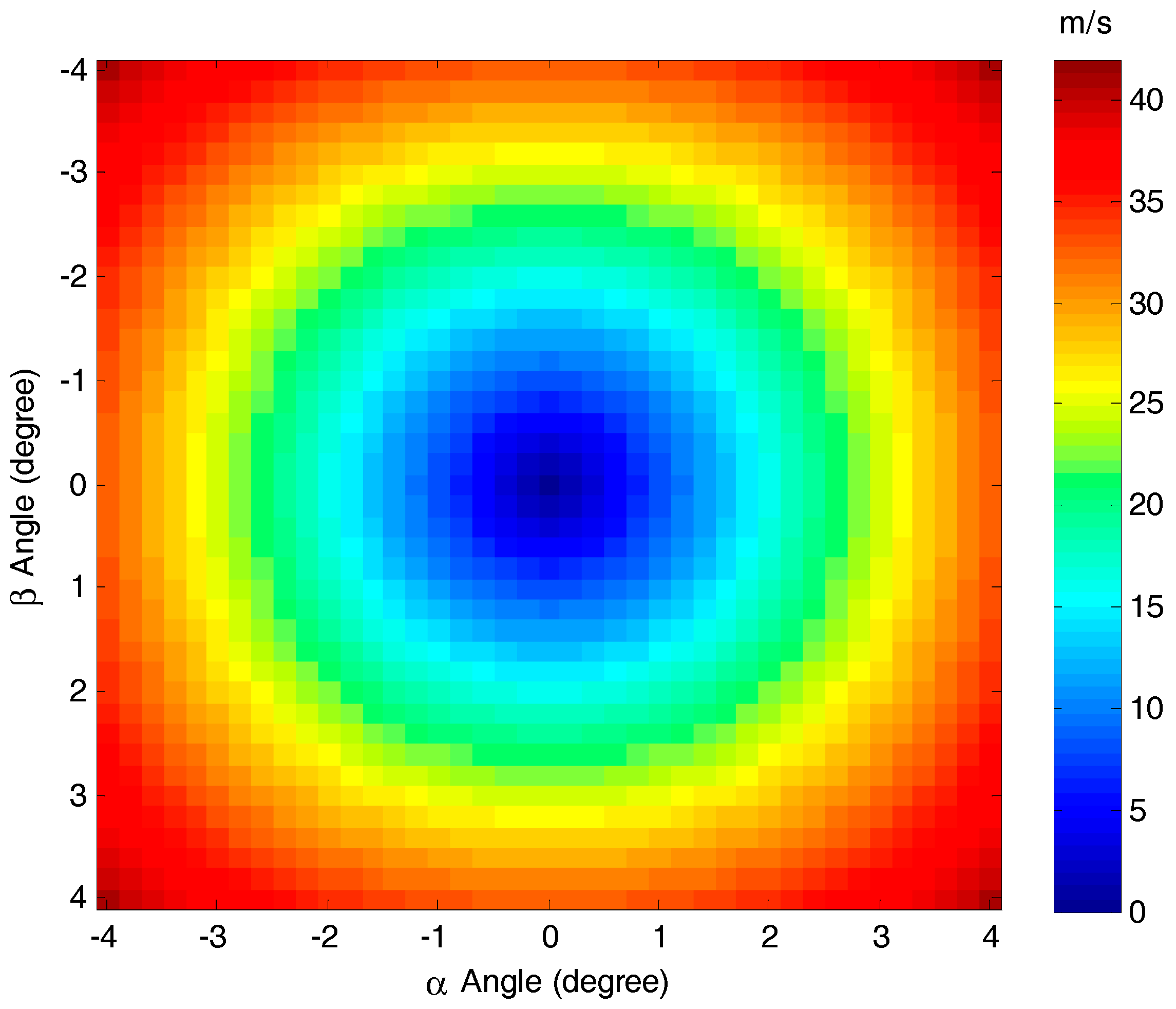
Figure 3.
Illustration of a frequency diversity pulse-pair (FDPP) pulse transmission mode. Two pulses at different central frequencies of f1 and f2 are transmitted with a time interval ΔT. Generally speaking, ΔT is relatively small, only taking a few μs or dozens of μs. The combination of four pulses is a complete pulse repetition time. The difference between f1 and f2 is usually a few MHz or the value of radar band. PRT is the complete pulse repetition time.
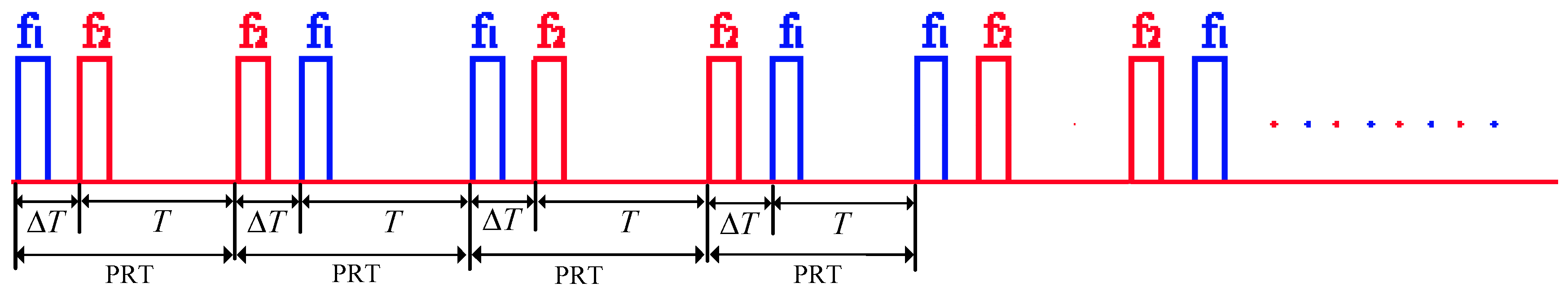
Figure 4.
FDPP algorithm phase estimation and velocity estimation. (a) Phase estimation of ΔΦR1 and ΔΦR2; the solid line indicates ΔΦR1 and dotted line indicates ΔΦR2; (b) the phase sum of ΔΦR1 and ΔΦR2 and (c) the velocity estimation; a dotted line indicates the unmodified velocity and solid line indicates the modified result of velocity estimation.
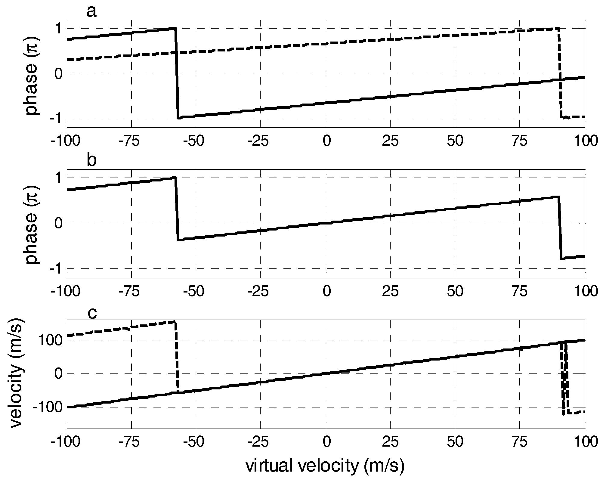
Figure 5.
The influence of PRF, the signal to noise ratio (SNR), and ΔT on the velocity estimation error. Velocity estimation deviation was determined with Monte-Carlo statistical tests for 1000 repetitions. (a) Velocity estimation error under different SNR; (b) velocity estimation error with different PRF and (c) velocity estimation error with different ΔT and SNR.
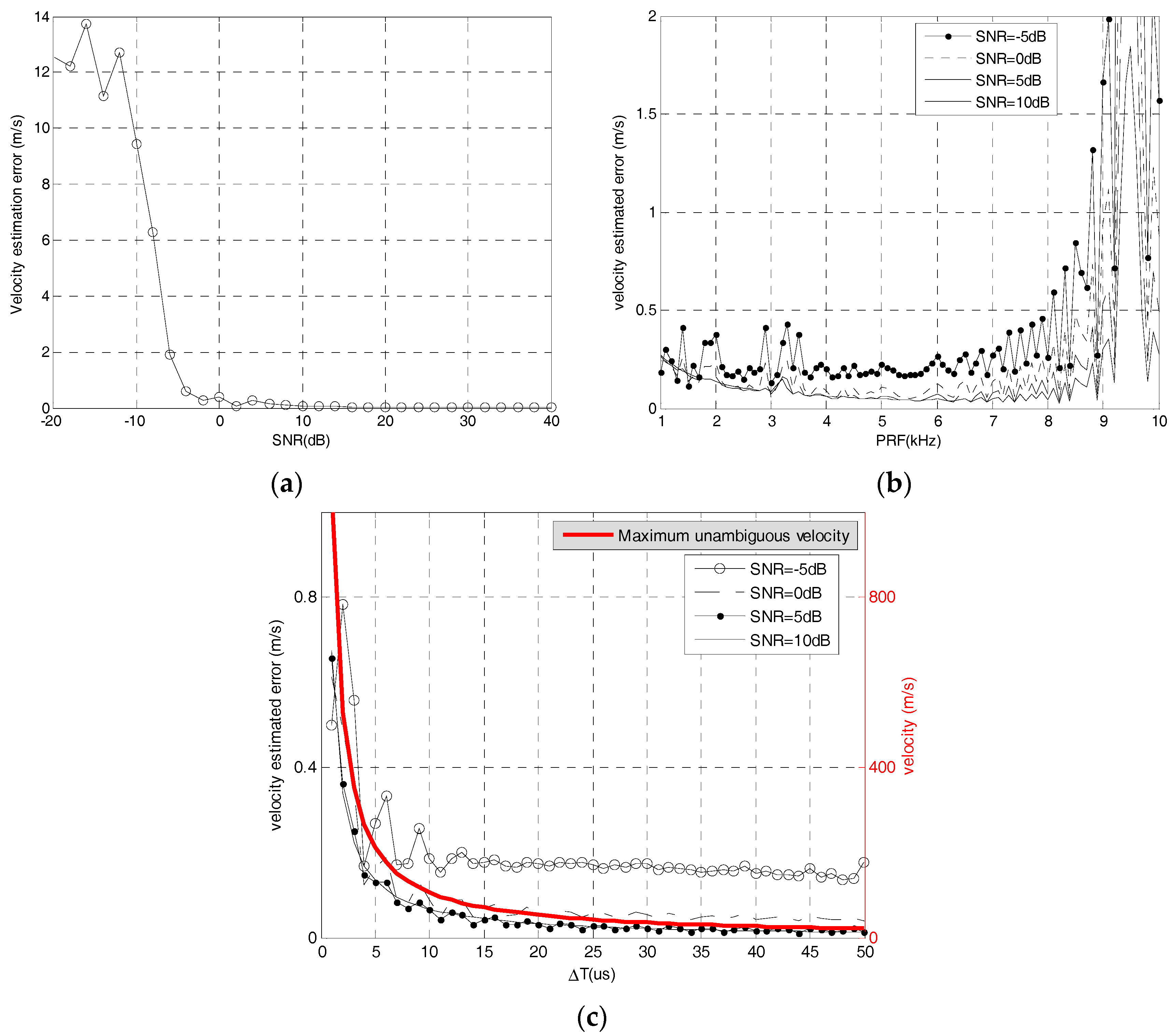
Figure 6.
(a) The spatial distribution of the precipitation particles model and (b) the antenna weighted and distance weighted schemes.
Figure 6.
(a) The spatial distribution of the precipitation particles model and (b) the antenna weighted and distance weighted schemes.
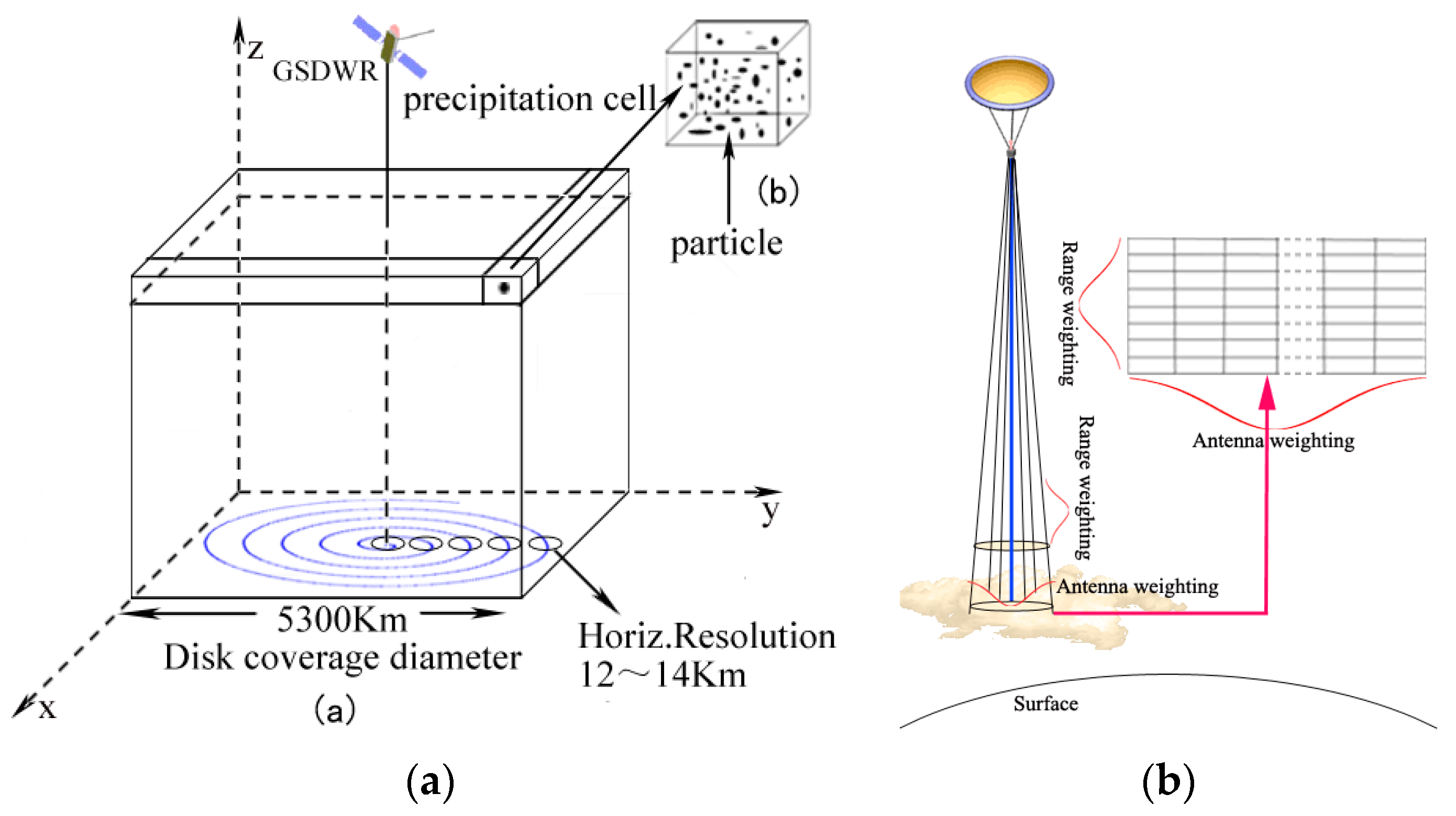
Figure 7.
(a) Flowchart of the simulation used to verify the FDPP algorithm; (b) reflectivity and velocity data of APR-2. The red rectangle A is one radial data region of GSDWR.
Figure 7.
(a) Flowchart of the simulation used to verify the FDPP algorithm; (b) reflectivity and velocity data of APR-2. The red rectangle A is one radial data region of GSDWR.
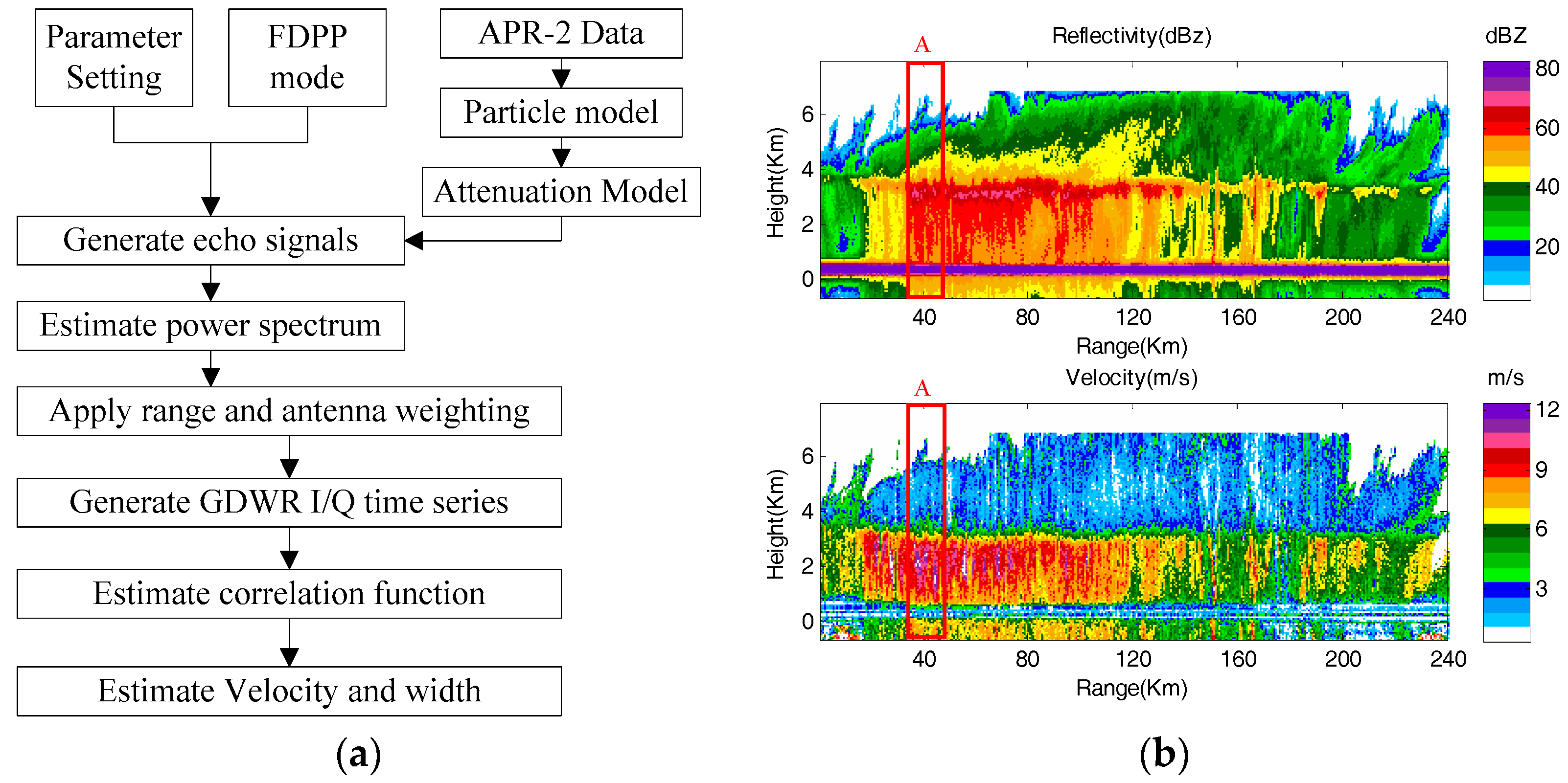
Figure 8.
FDPP velocity estimation and dealiasing results. (a) Comparison between FDPP and PPP velocity estimation results when PRF is 4000 Hz: the maximum unambiguous velocity is 8.5 m/s with PPP and 105.6 m/s with FDPP. The black line represents the estimation results; (b) Comparison between FDPP and PPP velocity estimation results when PRF is 1000 Hz.
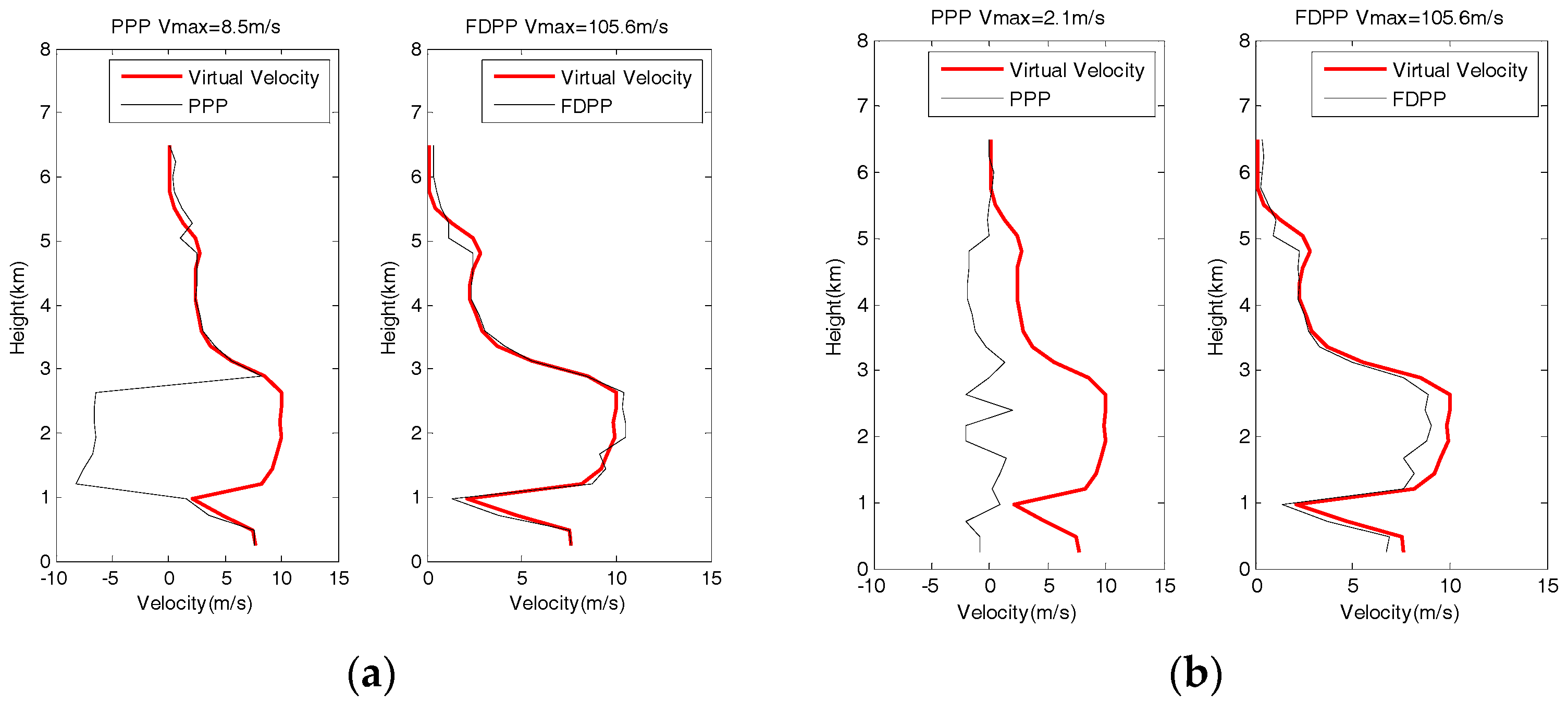
Figure 9.
Comparison of the results of two velocity estimation methods. (a) Velocity echo with PPP method and the real velocity of the elliptical region is greater than 8.5 m/s; the white part of the ellipse indicates the ambiguous region; (b) velocity echo with FDPP method and the velocity in the ellipse close to the virtual velocity.

Figure 10.
Velocity estimation bias and probability distribution of FDPP at different SNR. The red line in the scatter plots represents the zero-deviation standard, and the histogram indicates the probability of velocity bias being less than 0.5 m/s.
Figure 10.
Velocity estimation bias and probability distribution of FDPP at different SNR. The red line in the scatter plots represents the zero-deviation standard, and the histogram indicates the probability of velocity bias being less than 0.5 m/s.

Figure 11.
Velocity estimation bias and probability distribution of FDPP at different ΔT. The red line in the scatter plots represents the zero-deviation standard, and the histogram indicates the probability of velocity bias being less than 0.5 m/s.
Figure 11.
Velocity estimation bias and probability distribution of FDPP at different ΔT. The red line in the scatter plots represents the zero-deviation standard, and the histogram indicates the probability of velocity bias being less than 0.5 m/s.
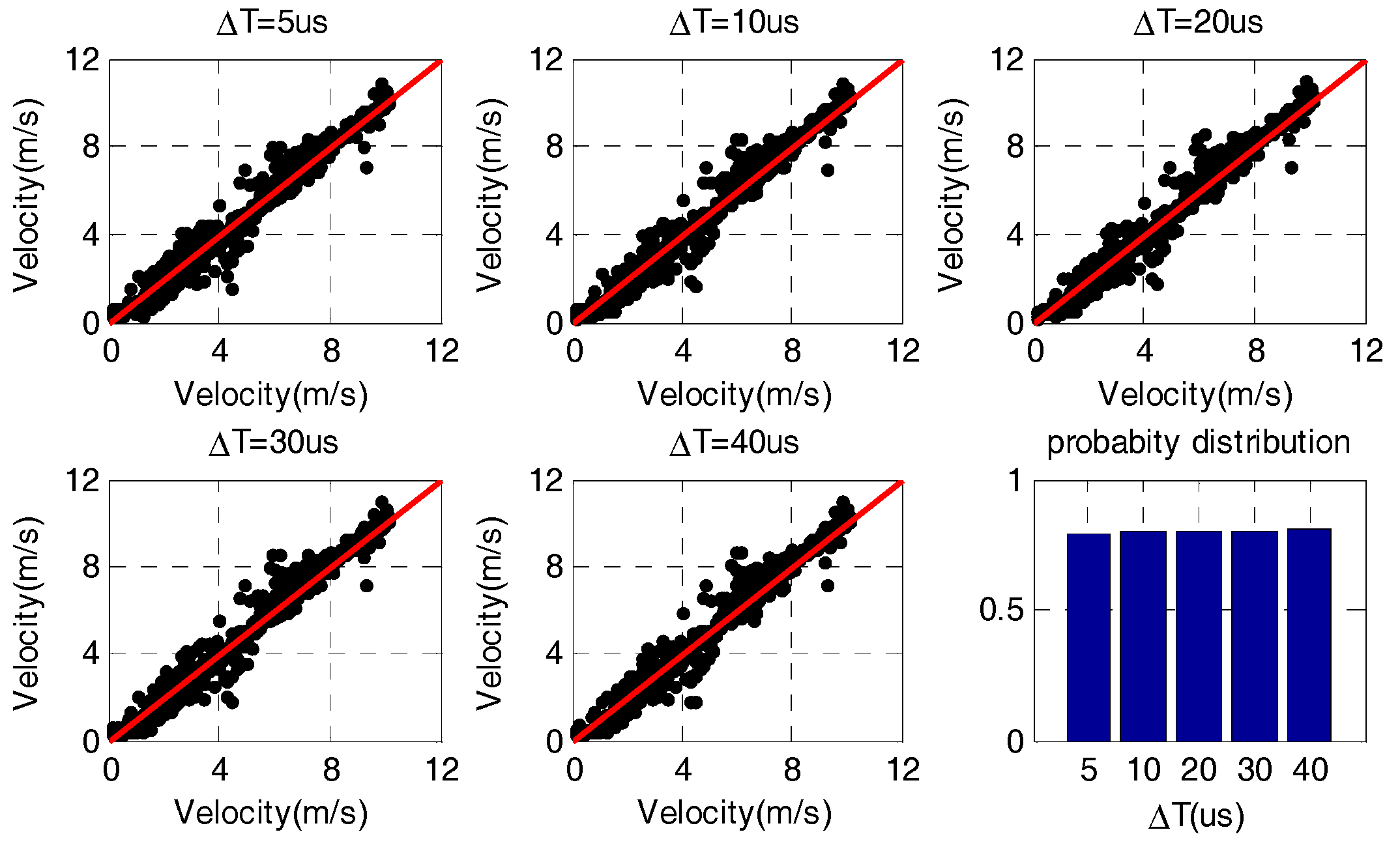
Figure 12.
Velocity estimation bias and probability distribution of FDPP at different PRF. The red line in the scatter plots represents the zero-deviation standard, and the histogram indicates the probability of velocity bias being less than 0.5 m/s.
Figure 12.
Velocity estimation bias and probability distribution of FDPP at different PRF. The red line in the scatter plots represents the zero-deviation standard, and the histogram indicates the probability of velocity bias being less than 0.5 m/s.
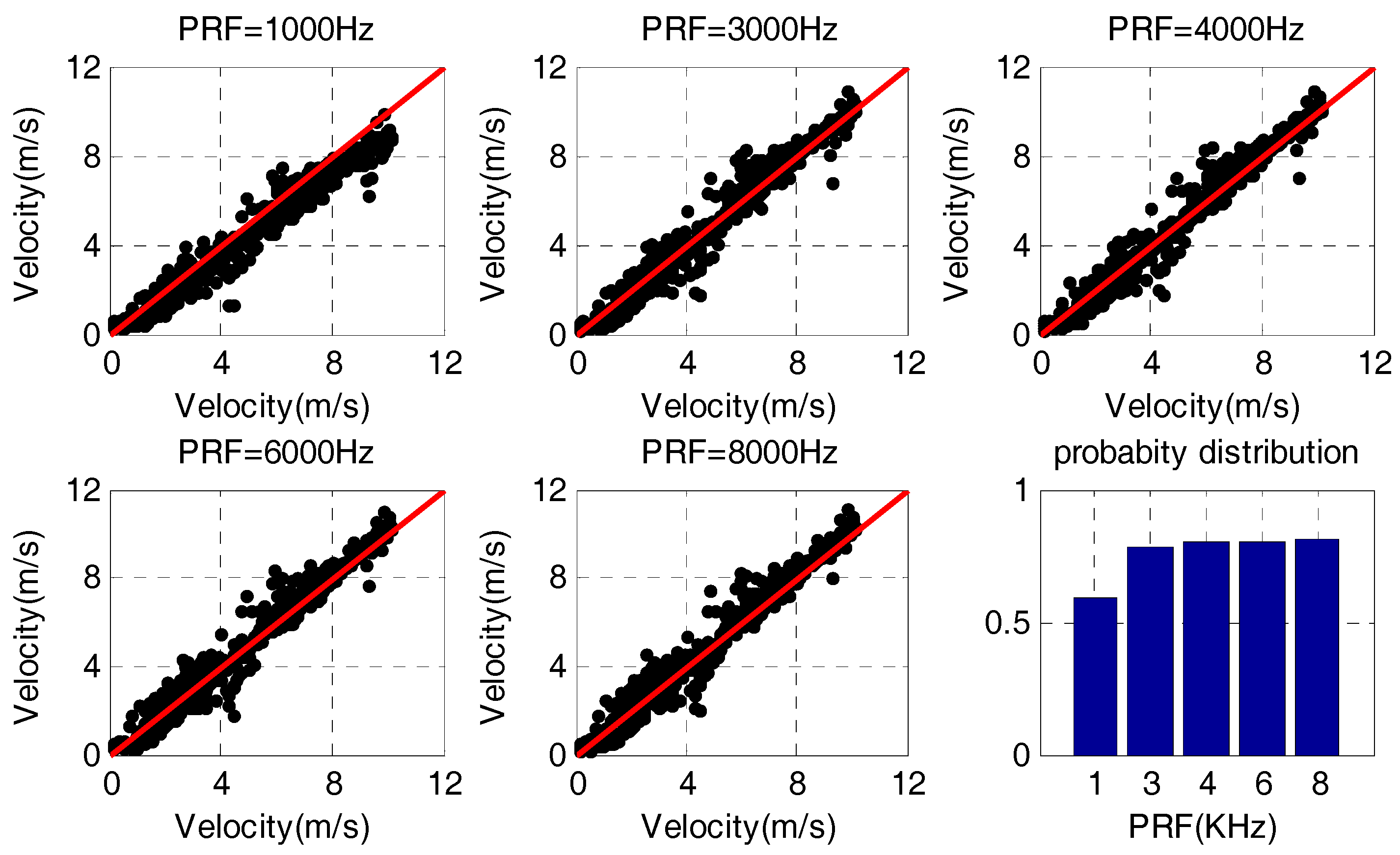
Figure 13.
(a) Velocity and spectrum width with FDPP estimation: the maximum spectral width is 4 m/s and most of the spectral width values are within the range of 0–2 m/s. Where the marginal part and the speed value change are obvious, and the velocity data and the velocity spectrum are relatively large; (b) Distribution characteristics of velocity spectral width. The X-axis represents the normal distribution characteristics of the theory, and the Y-axis represents the velocity spectrum width data. The red line represents the ideal distribution; the more data scattered closer to the red line, the closer the spectral width data is to the normal distribution.


Table 1.
Radar system parameters.
| Parameter | Parameter Value |
|---|---|
| Frequency | 35 GHz |
| Antenna diameter | 35 m |
| Time for a full scan | 60 min |
| Disk coverage diameter | 5300 km |
| Ant. 3-dB beam-width | 0.019° |
| Max. spiral scan angle | 4° |
| Dynamic range | 70 dB |
| Sys. Noise temp | 910 K |
| Doppler Precision | 0.5 m/s |
| Min. Zeq | 5 dBZ |
| Peak power | 100 W |
| Vertical Ranging range | 25 km |
© 2018 by the authors. Licensee MDPI, Basel, Switzerland. This article is an open access article distributed under the terms and conditions of the Creative Commons Attribution (CC BY) license (http://creativecommons.org/licenses/by/4.0/).
Share and Cite
MDPI and ACS Style
Li, X.; Wang, C.; Qin, Z.; He, J.; Liu, F.; Sun, Q. A Velocity Dealiasing Algorithm on Frequency Diversity Pulse-Pair for Future Geostationary Spaceborne Doppler Weather Radar. Atmosphere 2018, 9, 234. https://doi.org/10.3390/atmos9060234
AMA Style
Li X, Wang C, Qin Z, He J, Liu F, Sun Q. A Velocity Dealiasing Algorithm on Frequency Diversity Pulse-Pair for Future Geostationary Spaceborne Doppler Weather Radar. Atmosphere. 2018; 9(6):234. https://doi.org/10.3390/atmos9060234
Chicago/Turabian StyleLi, Xuehua, Chuanzhi Wang, Zhengxia Qin, Jianxin He, Fang Liu, and Qing Sun. 2018. "A Velocity Dealiasing Algorithm on Frequency Diversity Pulse-Pair for Future Geostationary Spaceborne Doppler Weather Radar" Atmosphere 9, no. 6: 234. https://doi.org/10.3390/atmos9060234
Note that from the first issue of 2016, this journal uses article numbers instead of page numbers. See further details here.